Reinforcement Learning Recommendation Algorithm Based on Label Value Distribution

Abstract

Reinforcement learning is an important machine learning method and has become a hot popular research direction topic at present in recent years. The combination of reinforcement learning and a recommendation system, is a very important application scenario and application, and has always received close attention from researchers in all sectors of society. In this paper, we first propose a feature engineering method based on label distribution learning, which analyzes historical behavior is analyzed and constructs, whereby feature vectors are constructed for users and products via label distribution learning. Then, a recommendation algorithm based on value distribution reinforcement learning is proposed. We first designed the stochastic process of the recommendation process, described the user’s state in the interaction process (by including the information on their explicit state and implicit state), and dynamically generated product recommendations through user feedback. Next, by studying hybrid recommendation strategies, we combined the user’s dynamic and static information to fully utilize their information and achieve high-quality recommendation algorithms. Finally, the algorithm was designed and validated, and various relevant baseline models were compared to demonstrate the effectiveness of the algorithm in this study. With this study, we actually tested the remarkable advantages of relevant design models based on nonlinear expectations compared to other homogeneous individual models. The use of recommendation systems with nonlinear expectations has considerably increased the accuracy, data utilization, robustness, model convergence speed, and stability of the systems. In this study, we incorporated the idea of nonlinear expectations into the design and implementation process of recommendation systems. The main practical value of the improved recommendation model is that its performance is more accurate than that of other recommendation models at the same level of computing power level. Moreover, due to the higher amount of information that the enhanced model contains, it provides theoretical support and the basis for an algorithm that can be used to achieve high-quality recommendation services, and it has many application prospects.

1. Introduction

As we are in the information explosion era of the Internet, to enhance users’ experiences of retrieving information and to reduce confusion surrounding different choices that are caused by information overload, recommendation systems have been widely used and have brought considerable convenience to people’s lives [1]. People are using the Internet at increasing rates, and many behavior logs and other data on their Internet use have been recorded. However, the Internet information stock is huge, effectively using it is difficult, and this results in information overload [2,3]. The purpose of a recommendation system is to help users screen the product information they may be interested in by analyzing the behavior characteristics of the users, and this is performed by using interaction behavior data on users and products. For example, more than 80% of movie viewing on Netflix is due to recommendation systems [4], and more than 60% of the videos watched on YouTube are accessed via the homepage recommendations [5,6]. Interacting with the recommendation system can not only continuously enhance the user’s interaction experience, but it also has remarkable commercial value for relevant trading platforms [7,8].

The first recommendation systems to be applied on a large scale were user-based collaborative filtering systems, such as Tapestry’s email filtering system in the 1990s [9] and GroupLens’ introduction of collaborative filtering into the news field [10]. In 2003, Amazon invented the item base collaborative filtering method, which solved the problem of the user bases having a high time complexity [11]. Breese et al. (1998) proposed a model-based system filtering method that has been widely used because of its domain-independent characteristics [12]. Pazzani (1999) proposed a content-based recommendation algorithm that directly calculates the similarity of items through metric learning; this is performed by calculating the interaction information between users and items, and the algorithm can be used to solve the cold start problem [13].

Deep learning can also be used to efficiently and accurately process recommendation tasks, and it has become an important direction for recommendation system research [14]. Regarding the application of neural networks in recommendation systems, He et al. (2017) proposed a neural collaborative filtering algorithm that can be used to extract the nonlinear relationship between users and items [15]. Hidasi et al. (2016) proposed a session-based RNN recommendation model that takes the coding of items as the input and predicts the possibility of each item being clicked by the user according to the user’s browsing history [16]. The combination of deep learning and recommendation technology has broad development prospects, and various recommendation systems that combine deep learning have emerged and are endless. Regarding recommendation systems that are sensitive to the freshness of the data, obtaining satisfactory results by using static methods is difficult. In this case, creating recommendations by using reinforcement learning is obviously more effective than using pure static methods is.

A commonly used method is the upper confidence bound algorithm. The disadvantage is that this method is context free [17]. Yahoo! scientists solved this problem and applied the LinUCB algorithm to Yahoo!’s news recommendations, and the characteristics of the users and items were considered. Because more information is used, its performance was greatly enhanced compared to that of UCB [18]. In recent years, reinforcement learning has been increasingly developed by scholars, and its combination with recommendation systems has also received a plethora of attention; as a result, this combination has become an important research direction for recommendation systems.

Collaborative interactive recommendation systems have gradually developed with the vigorous development of the recommendation system field. Scholars involved in both theoretical research and industry practice have proposed that recommendation systems must meet higher requirements before they can interact with users in a complex manner, and researchers have gradually developed a system that can explore users’ interests across multiple dialogue rounds [19,20,21,22,23,24,25,26]. The term collaborative interactive recommenders (CIRs) defines a recommendation system that can engage in multiple rounds of collaborative exploration with users to more accurately meet their needs [27]. CIRs usually use conversations to maximize user participation and satisfaction through a series of interactions. Because the risk and cost of directly using new algorithms to test CIRs on commercial platforms are very large, using a configurable interactive recommendation simulation environment for algorithm evaluations and experiments is of considerable practical importance. Currently, several popular configurable interaction platforms exist. The RecoGym platform is an interactive recommendation simulation system that is mainly used in the e-commerce industry. Its advantage is that data are generated from real data through desensitization modeling, so the authenticity of the platform’s data is relatively high. The disadvantage is that it is a relatively fixed industry-direction platform, and some new interaction forms do not support it or user-state transitions. The RecSim platform is an interactive recommendation simulation system released by Google that defines user states in any complex form and changes the definition of observable states for recommenders. Its disadvantage is that configuring a reasonable environment requires a large amount of expert knowledge or real data, as it otherwise does not have the credibility of using real data. The RecSim NG platform can be used to create transparent and configurable end-to-end recommendation ecosystem models, and it provides a set of methods to evaluate recommendation ecosystems when combined with the behavior models of other entities.

The optimization objectives of recommendation systems are mainly divided into the regression problem of scoring [8] and the ranking problem [28]. However, although machine learning and big data methods have greatly promoted the development of recommendation systems, problems concerning the interpretability of the models [29] as well as the cold start [30,31] and static model problems [32,33] still exist. The performance of traditional recommendation systems has gradually failed to meet the various needs of people. More recommendation models that can handle nonlinearity have emerged. An important research direction is the application of reinforcement learning in recommendation systems. The authors of most previous works have been limited to processing nonlinear information, such as by using tree models, deep learning, kernel methods, and so on to deal with nonlinearity in the data. The nonlinear data are transformed into a linear space, and then a linear model is used for discrimination or regression. This method is usable when using complete information, but in actual scenarios that the recommendation system is used in, the expectations that the model needs to deal with are also nonlinear when modeling with incomplete information. Therefore, determining how to introduce such nonlinear expectations into reinforcement learning algorithms and conducting innovative explorations with the recommendation system and from the perspective of engineering practice is our focus. We used methods such as value distribution reinforcement learning and label distribution learning on data from e-commerce simulation environments and user characteristics to design a recommendation algorithm that can balance multiple factors and meet user needs to the maximum extent, which will provide users with high-quality recommendation services. Our main contribution is the integration of nonlinear expectations into the design and implementation process of recommendation systems, which will allow recommendation systems to efficiently use user behavior information.

2. Research Design and Model Construction

2.1. Fuzzy Mahalanobis Metric Clustering Enhancement

Fuzzy Mahalanobis metric clustering is used to enhance fuzzy C-means (FCM) clustering. The $n$ vector ${\overrightarrow{x}}_i$ is divided into $c$ fuzzy clusters. The membership degree $u_{i,j}$ represents the uncertainty and the membership degree of sample $i$ to class $j$.

$${\displaystyle \sum _{i=1}^c{\displaystyle \sum _{j=1}^n{u}_{i,j}}}=1$$

(1)

Here, $U$ is the membership matrix, $c_i$ is each centroid, ${\lambda }_j$ is the weighting index, and the final objective function is

$$\begin{gathered} J(U,c_1,\cdots c_c;{\lambda }_1,\cdots {\lambda }_n)=J(U,c_1,\cdots ,c_c)+{\displaystyle \sum }_{j=1}^n{\lambda }_j({\displaystyle \sum }_{i=1}^c{u}_{ij}-1) \\ ={\displaystyle \sum }_{i=1}^c{\displaystyle \sum }_{j=1}^n{u}_{ij}^m{d}_{ij}^2+{\displaystyle \sum }_{j=1}^n{\lambda }_j({\displaystyle \sum }_{i=1}^c{u}_{ij}-1) \end{gathered}$$

(2)

In Formula (2), $d_{i,j}$ represents the distance calculation, which is conducted by using the Euclidean distance calculation of the FCM. Once can replace the formula with the Mahalanobis distance and find the partial derivative of the center of mass, $c$, of the objective function to obtain Formula (3):

$$c_i=\frac{{\displaystyle \sum _{j=1}^n{u}_{ij}^m{x}_j}}{{\displaystyle \sum _{j=1}^n{u}_{ij}^m}}$$

(3)

Formula (4) can be obtained by finding the partial derivative of the fuzzy matrix of the objective function:

$$u_{ij}=\frac{1}{{\displaystyle \sum _{k=1}^c{(\frac{d_{ij}}{d_{kj}})}^{2/(m-1)}}}$$

(4)

The membership matrix and centroid calculated by the fuzzy Mahalanobis metric clustering algorithm can be used as the basic part of the model so that the sampling can have more intuitive and quantitative validity. The advantage of the Mahalanobis distance measurement over the Euclidean distance measurement is the dimension processing. Therefore, compared to the Euclidean distance determined by the actual calculation, this algorithm can calculate the distribution of the user characteristics. Therefore, sublinear coding is more effective when using this algorithm than the Euclidean distance because it can be directly used to calculate the sublinear coding as a clustering method.

2.2. Sublinear Coding Enhancement

The existing coding of each user can be decomposed by SVD to obtain the feature root, which is combined with the obtained sociological attributes of the user to become the linear coding of the user. However, the sublinear coding of the user that is calculated by using distributed learning and nonlinear expectation methods can more accurately represent the user’s interests and hobbies in the recommendation system, so an enhanced sublinear coding method is designed to enhance the description of the static information of the user.

First, the expectations represented by sublinear coding are defined:

$$E\widehat{}[x]:=\underset{\theta \in \Theta }{\sup }{}_{p_{\theta }}[x]$$

(5)

$E[•]$ is a functional of random variables and has monotonicity, constancy, nonlinearity, and positive periodicity. According to the actual situation, the functional has convergence when it is non-negative and downwardly approaches 0.

According to the nonlinear LLN (law of large numbers), $\{x_i\}$ is assumed to be an i.i.d sequence, and $\overline{\mu }=E\left[X_1\right],\underset{\_}{\mu }=-\left[-X_1\right]$ is assumed for each $f\in C_{lip}(R)$.

Regarding the uncertainty problem, sampling with the Monte Carlo method is important for computer simulations to obtain results. The calculation method is shown in Formula (6):

$$Mx[\phi ]:=\underset{n\to \infty }{\lim }\sup [\phi (x_1)+\cdots +\phi (x_n)]$$

(6)

Using the group sampling Monte Carlo method to calculate the maximum expected distribution can accelerate the convergence speed of the calculation. The calculation method is as follows:

Assuming that ${\{X_i\}}_{i=1}^{n\times m}$ is independent and identically distributed nonlinear data, by using the maximum mean method, it can be estimated as

$$\widehat{M}\left[\varphi \right]=max\{Y_n^k:k=0,\cdot \cdot \cdot ,m-1\}$$

(7)

where $Y_n^k$ is defined as

$$Y_n^k=\frac{1}{n}{\displaystyle \sum _{i=1}^n\varphi (X_{nk+i})}$$

(8)

According to the law of large numbers, when $\mathrm{n}\to \infty$, ${\{Y_n^k\}}_{k=0}^{m-1}\stackrel{d}{\Rightarrow }ani.i.d{\{Y_{}^k\}}_{k=0}^{m-1}$ and $Y^k\stackrel{d}{=}{M}_{[\underset{\_}{\mu },\overline{\mu }]}$, and this is expressed in the following Formula (9). Then, the risk functional can be calculated by using the $M{M}_X$ method of Formula (9), and the maximum group average of the nonlinear i.i.d samples can be calculated by using the nonlinear Monte Carlo method:

$$\begin{array}{l}max\{\underset{Y_n^0}{\underbrace{\frac{\varphi (X_1)+\cdots +\varphi (X_n)}{n}}},\dots ,\underset{Y_n^k}{\underbrace{\frac{\dots }{n}}},\dots ,\underset{Y_n^{m-1}}{\underbrace{\frac{\varphi (X_{(m-1)n+1})+\dots +\varphi (X_{mn})}{n}}}\}\\ E \left[\varphi (X)\right]\cong Max-Mean\left[\varphi (\{X_i\})\right]\\ M{M}_X\left[\varphi \right]:=\underset{0\le k\le m-1}{max}\frac{{{\displaystyle \sum }}_{i=1}^n\varphi X_{kn+i}}{n}\end{array}$$

(9)

Then, the sublinear expectation of the measure can be obtained with Equation (10):

$$E \left[f(x_1)-y_1{|}^2\right]=\underset{k\in \left[0,\cdots ,n-1\right]}{max}\{\frac{1}{m}{\displaystyle \sum }_{i=mk+1}^{mk+m}|f(x_i)-y_i{|}^2\}$$

(10)

where $y$ corresponds to the real value and $f$ can be obtained through neural network training and optimization.

$$f=\arg \underset{f\in F}{min}\underset{k\in \left[0,\cdots ,n-1\right]}{max}\{\frac{1}{m}{\displaystyle \sum }_{i=mk+1}^{mk+m}|f(x_i)-y_i{|}^2\}$$

(11)

The training complexity of the model is higher than that of the linear calculation because two termination conditions exist for the operation; one is that the model converges to a certain threshold, and the other is that the model runs to the maximum number of running rounds that set the super parameters. For this model, the running complexity of each round was M times higher than that of the linear model on a year-to-year basis. However, because the convergence nature of the model determines the number of running rounds, its theoretical convergence can be proven; the oscillation during model training is smaller than that of the linear model, and the number of running rounds is lower under the same circumstances. Therefore, the time complexity of the operation is almost at the same level or slightly higher by several times, and the details will vary depending on the data.

2.3. Enhancement of Contextual–Quantile Regression Reinforcement Learning Model

The distributional DQN is equivalent to the DQN expansion, which creates a reinforcement learning direction; that is, our cognition is expanded from the Q value to the Q distribution. The reinforcement learning model is enhanced by the distributed DQN to match the reinforcement learning method of the recommendation system. The purpose of the modification is mainly to increase the efficiency with which the model utilizes the data because although the offline data of the recommendation systems are very large, and the data used to solve the cold start problem and to support the interactive recommendation simulation system are very scarce. Moreover, because the recommendation system itself has relatively complete control of and characterizes the environment, scholars recommend using model-based methods to increase the data analyzing efficiency when using the reinforcement learning method in the recommendation system.

The quantile regression reinforcement learning model is context-free. If this algorithm is only applied to the recommendation system, it cannot use the context information of the recommendation scene. For all users, the strategy of presenting goods is the same, and this cannot meet the personalized requirements of the recommendation system. Therefore, the applicability of the contextual–quantile regression reinforcement learning model needs to be enhanced.

The random process is redefined as $(C,X,A,P,R,\gamma )$ where $X$ and $A$ are the state and action space, respectively, and $X$ is the context feature of the user. $P(•|c,x,a)$ is the state transition matrix, $\gamma$ is the discount factor, and $P$ is the return function.

Suppose that the current step is $t$; the current user is $u_t$; and the observable feature vectors of each selectable product $a$ are $c_u$ and $x_{t,a}$, which contain the user’s static and dynamic information and product information. According to the results observed before, $a_t$ is selected to return. The return expectation depends on the user’s static and product characteristics, list order, and other dynamic characteristics. The neural network enhances its product recommendation strategy according to the new observation $(c_u,x_t,a_t,r_{t,a}{}_t)$, and the goal of the whole process is to minimize the loss in the whole process, which is the regret value.

$$R_A(T)=[{\displaystyle \sum _{t=1}^T{r}_{t,a_t}^{*}}]-[{\displaystyle \sum _{t=1}^T{r}_{t,a_t}^{}}]$$

(12)

Because the expectation of model processing depends on a variety of aspects, the information on each aspect may be incomplete or inaccurate, and the selection of actions is related to the historical context of the user; additionally, the expectation is nonlinear, and the distribution form is used to represent this nonlinear expectation. Algorithm 1 shows the algorithm logic of the contextual–quantile regression reinforcement learning network.

Algorithm 1: Contextual–Quantile Regression Reinforcement Learning Network

$\mathrm{Hyperparameter}:N,K$

$\mathrm{Input}:c,x,a,r,x^{\prime },\gamma \in [0,1)$

# Computational distribution Bellman operator

$Q(s^{\prime },a^{\prime }):={\displaystyle \sum _j{q}_j{\theta }_j}(c,x^{\prime },a^{\prime })$

$a^{*}\leftarrow \arg \underset{a^{\prime }}{\max }(c,x,a^{\prime })$

$T{{\theta }^{\prime }}_j=r+\gamma {{\theta }^{\prime }}_j, i=0,1,\cdots N-1$

# Optimized quantile regression loss

$\mathrm{Output}:{\displaystyle \sum _{i=1}^N{E}_j[{\rho }_{{\widehat{\tau }}_i}^{\mathrm{K}}(\tau {\theta }_j-{\theta }_i(c,x,a))]}$

3. Experimental Design and Environmental Configuration

3.1. Encryption Algorithm Description

3.1.1. Platform Selection

Unlike the traditional recommendation system that is concerned with static users, CIRSs (community information and referral services) need a training platform that can support simulation interactions so that the model can learn the sequential pattern of the users’ behavior during the interaction process.

Therefore, the selected simulation platform has the following characteristics: the environment considers the user’s natural browsing behavior and the commodity interaction behavior of the user; the platform includes the association definition of user behaviors at the parameter level; after users and commodities are clustered, the hidden space dimension can be parameterized; and the platform allows for the parameterization of the relative impact of the user’s past exposure level on the ad display click through rate at a given time. Taking the e-commerce CTR as an example, we selected the RecoGym platform to train the model. The goal of the agent was to display personalized advertisements, encourage users to access or return to e-commerce websites, and increase the click through rate of user advertisement pairs. The Markov process of user browsing and interactive session is shown in Figure 1.

3.1.2. Parameter Setting

The composition definitions of the environment are shown in

Table 1. Definitions of environmental composition.

Name	Definition
P	Quantity of items
u	User
t	From the beginning of the session to the current time
Zu,t	Current transaction type (enumeration type: organic or bandit)
Vu,t	User browsing item ID. If it is bandit, it is none
au,t	Item recommendation action. If it is organic, it is none
Cu,tt	Whether a click event occurs. If it is organic, it is none

.

According to the definitions in Table 1, the actual modeling environment can be set, as shown in

Table 2. Environmental modeling parameters.

Name	Symbol Interpretation	Model Definition	Value
K	Late factor dimension	K	50
P	Item quantity	num_products	1000
F	Difference between organic and bandit	number_of_flips	650
µt	Average visit duration	normal_time_mu	1
σt	Access to the box difference during stay	normal_time_sigma	1
σ(µ)	Potential characteristic difference in user interest	sigma_mu_organic	2
σ(ω)	Initialization of potential features of user interest	sigma_omega_init	1
	Noise	sigma_omega	0.2
	Does omega change with interaction	change_omega_for_bandits	True

.

We obtained a set environment by setting the above parameters. This environment had the following characteristics: users’ interests will slowly shift, the access time of the user is related to the latent variable of interest, a long tail effect in the users’ behavior is present, and the latent variable of the users’ interest is unobservable.

3.1.3. Data Description

The data used were divided into two parts: the users’ browsing data and users’ interaction data. The browsing and interactive data had different formats, and they were uniformly formatted into a table and displayed as a log. The format is shown in

Table 3. Data format description.

Name	Function Description	Related Matters	Value Range
t	Serial value or time	None	Serial value: int, time: float
u	User ID	None	Int
z	Interactive identification	Enumeration type	Browse: organic, interact: bandit
v	Browse item identification	None in bandit	Int
a	Action	Products displayed to users	Int
c	User feedback	Whether the user provides positive feedback	User click: true, no action: false
ps	User click probability	None in organic	0–1
ps-a	All action probabilities	None in organic	0–1

.

We used logs of 10,000 users to analyze the data and obtain relevant statistical information. In total, we obtained 1,004,594 log data, including 778,538 interactive data. From these, we could see the exposure of each product in the exploration stage, with an average of 778.538 and a standard deviation of 28.159. From the distribution of its actions (recommended products), we could see that the exploration actions were random. In the historical records, this met the random condition. All the actions were randomly applied to all reinforcement learning events. According to the statistics obtained on the interaction records of the users, the average interaction length was 77.854 and the standard deviation was 79.336. The interaction length of different users was different, with a range of 683. The shortest was only 1 and the longest was 684. The segmentation data of the user interaction length are shown in Figure 2.

Figure 2 shows that most people engaged in interaction behaviors less than 200 times. Most of the users’ data were sparse, and only a few users interacted with the recommendation system more than 500 times. Therefore, huge differences in the interaction behavior and the number of interactions existed across different users.

The differences can be more intuitively seen in the click through rate indicators of the different users. As can be seen in Figure 3, the click through rate indicators of the users were divided into boxes according to the number of exploration behaviors, and the corresponding distribution of the users in the boxes was visualized with a violin chart. The following conclusions could be drawn from the analysis of Figure 3:

(1)

If users have more interactive behaviors, their click through rate indicators are relatively stable and remain at the same level.

(2)

If the number of user interaction behaviors is higher, the click through rate indicator is higher in the case of random recommendations.

(3)

If the number of user interaction behaviors is too few, the variance is abnormally large, which should be considered an invalid interaction and eliminated during actual processing. In the case of insufficient information, the quality of the output training samples is not high, which will affect the model fitting.

3.2. Experimental Environment Configuration

3.2.1. Hardware Configuration

The hardware configuration used in this experiment is shown in

Table 4. Hardware configuration.

Hardware	Model	Quantity
CPU	Intel E5-2650 V3	2
Memory	32 G	4
Hard disk	RAID5 3 T	3
Graphics card	NVIDIA Tesla M40 24 GB	1

.

3.2.2. Software Configuration

The software configuration used for this experiment is shown in

Table 5. Software configuration.

Environment	Edition
Operating system	Ubuntu 16.04 Server
Python	3.6.15
Pytorch	1.2.0
RecoGym	0.1.3.0
Hadoop	2.7.2
Hbase	1.2.1
Hive	2.3.X
Spark	3.1.2
Pig	0.13.0

.

3.2.3. Resource Demand

The experiments were divided into a function and index verification and a performance test. We used different data levels for different experiments. Among them, the purpose of function verification was to quickly verify the function of the data and to determine the effect of the model when a small amount of data were used, whereas the purpose of index verification was to verify the relevant indicators of the model with larger-scale data; to facilitate the experiments, the operation time was controlled within days. The purpose of the performance test was to verify the stability, feasibility, and time complexity of the model with a large amount of data and to test the stability of the overall recommended system environment. The amount and level of data required for tests of a different nature and the resources required for the experiments were also different. The resource requirements are shown in

Table 6. Resources required for different experiment types.

Experimental Nature	Number of Test Items	Number of Test Users	Memory Usage	Offline Data Volume
Functional verification	1000	10,000	Less than 2 GB	About 1,004,594 articles
Indicator verification	1000	50,000	Less than 2 GB	About 5,118,051 articles
Performance testing	5000	100,000	No more than 4 GB	About 10,104,289 articles

.

The above data were automatically generated by the RecoGym platform. After the data were generated and stored in a file, they were outputted in a table by Hive. Then, a distributed calculation was conducted within the data. After grouping and aggregation, the calculation was completed and stored in a new Hive table, and the calculated data were converted into a CSR sparse matrix by another program.

4. Experimental Verification and Result Analysis

4.1. Establishment of Recommendation Algorithm Evaluation Indicators

The model evaluation indicators that we propose are mainly from an economic perspective. The $CTR$ (click through rate) and $HR@K$ ($HR$ is the hit ratio) are the main indicators; the $CTR$ indicator is an indicator that is directly related to commercial realization, and $HR@K$ is an evaluation index of user stickiness. These indicators can reflect the health status of the whole system and the effectiveness of the model and can provide more effective training data for subsequent model optimization.

The $CTR$ indicator, that is, the click through rate indicator, is an important indicator with which to measure the recommendation effect in the field of Internet advertising and recommendation systems. In actual operation, this indicator is an important measure of the platform economy. If an interaction process is defined as a tuple, where the options are is action, is context, and is return, then the $CTR$ value can be calculated from Equation (13) to determine the logging policy:

$$CT{R}_{{\pi }_t}(\mathrm{L})=\frac{-}{\left|\mathrm{L}\right|}{\displaystyle \sum _{(a,x,c)\in \mathrm{L}}c\frac{{\pi }_t(a|x)}{{\pi }_l(a|x)}}$$

(13)

The $Hit-Rate@K$ (abbreviated as $HR@K$) indicator is a commonly used evaluation indicator of the recommendation system. It is defined as the ratio of the number of users and the total number of users whose products appear in the Top-K recommendation list in the test set. $HR@K$ is used to measure how accurate the model is at predicting user behavior. Its value can be calculated by using Equation (14):

$$HR@K=\frac{NumberofHits@K}{\left|GT\right|}$$

(14)

4.2. Validation Experiment of Static Features

The purpose of conducting the effectiveness verification experiment on the user’s static features was to verify the effectiveness of the user’s feature engineering. Because the feature engineering contains nonlinear information, the preconditions of most statistical testing methods were not satisfied. Here, the experiment was verified by conducting a comparative experiment under the same environmental conditions.

The commonly used random forest model was selected as the baseline test model for the experimental model. The data input into the model were processed by using different feature engineering methods, and different feature engineering processing methods were used as variables. The results output from the model were horizontally compared. The feature processing methods were as follows:

(1)

A feature engineering method based on counting, which simply counted the data to calculate the browse and interaction quantity of each product as the baseline method for comparison.

(2)

A feature engineering method based on SVD decomposition: the hidden code length level of the SVD was set at 5, 20, and 50 levels, and the codes were svd-5, -20, and -50, respectively.

(3)

A feature engineering method based on simple sublinear coding: the levels of the number of users (M) were 50, 150, 500, and 5000, and the codes were SubLinEmb-50, -150, -500, and -5 k, respectively.

(4)

A systematic design based on the user’s static characteristic data: When processing the data, the information contained within the data was cleaned, converted, and processed. After the processing was completed, the data were cached in the memory system until the near-line and online applications. The code name was Entirety-Plan.

The environmental parameters of the experiments were constructed and presented in Table 2, by using two indicators in CTR, i.e., HR@5 and HR@2, to measure the performance of the model algorithm.

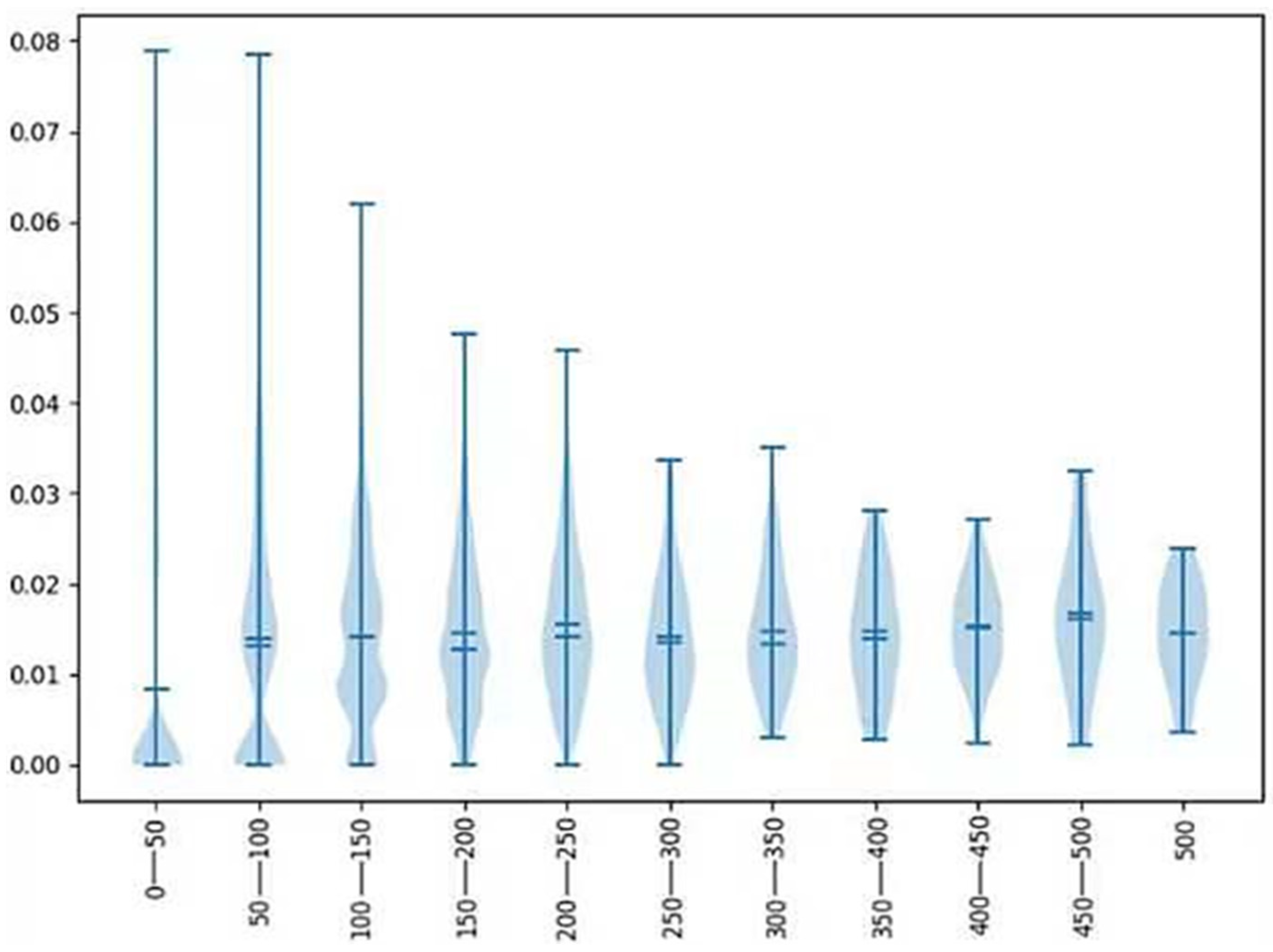
The comparison results are shown in Figure 4, where the middle dot represents the mean value and the line segment represents the standard error. The general information level included in the feature engineering process can be seen. The following conclusions can be drawn from the results:

First, the increase in the hidden variables of feature engineering based on SVD can enhance the effect of HR@5. When 200 dimensions were present, the indicator was enhanced, but the enhancement was limited.

Second, sublinear coding was more accurate than feature engineering was based on SVD. More neighbor samples will not enhance the effects, and too many neighbors will introduce redundant data, which will have the opposite effect.

Third, for many product recommendations, the effect of popular product recommendations and random recommendations was almost zero.

Fourth, the scheme that combined linear and sublinear and sequential patterns was optimal, which was not unexpected because the scheme was based on the most comprehensive information.

Regarding HR@5 and, correspondingly, HR@2, the result was very similar to that in Figure 3. At the same time, compared with the HR@5 data, the HR@2 value was slightly worse.

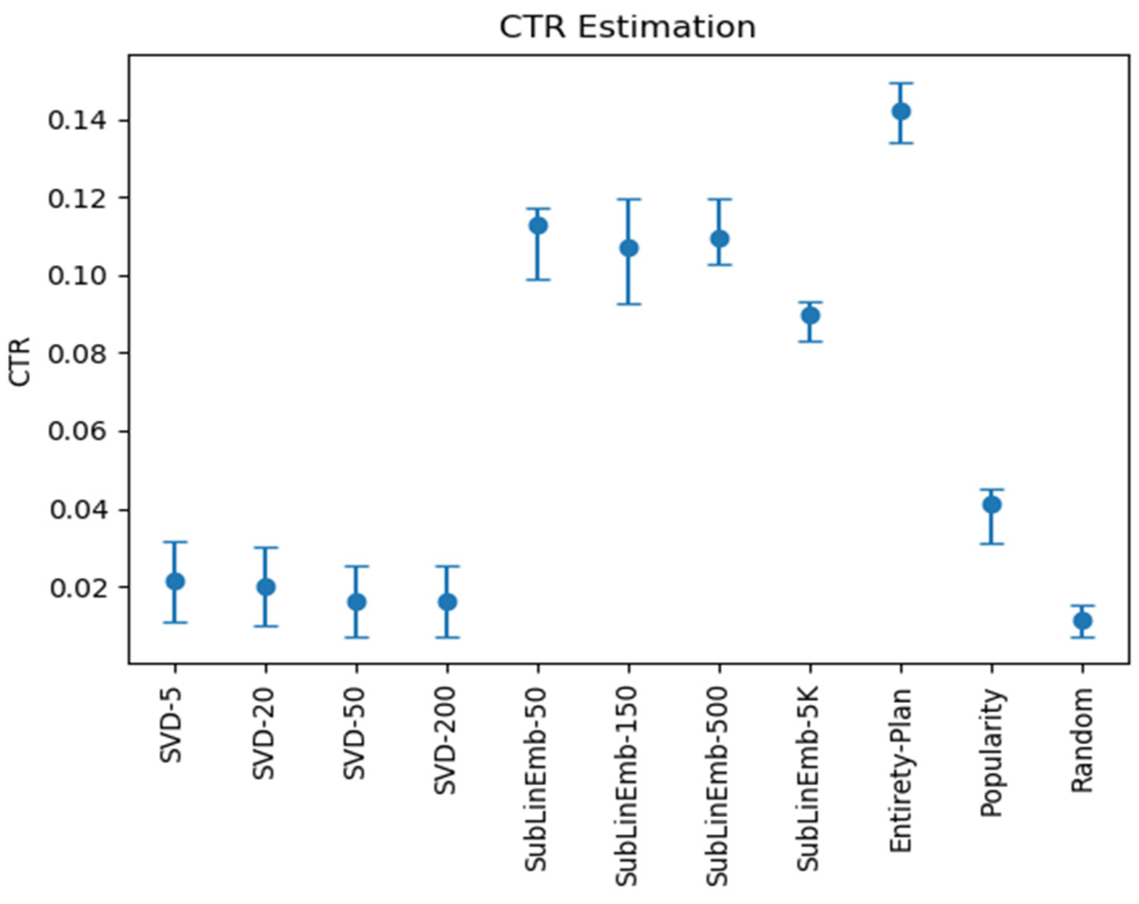
The control results of the CTR are shown in Figure 5. From the CTR indicators, we found the following:

(1)

Increasing the number of implicit variables will not enhance the index, but it will decrease the performance of the index.

(2)

As a baseline model, the effect of the popularity recommendation was stronger than that of SVD, but the effect was not very strong overall. The random recommendations were the worst, which we were expecting.

(3)

The feature engineering method using sublinear coding was much more effective than the linear SVD correlation method was because it considered this situation in theory.

(4)

The scheme that combined the linear and sublinear and sequential patterns as a whole was optimal, which was not unexpected because it had the most comprehensive information.

From the results of the above experiments, we found that introducing a method to add nonlinear expectations into the recommendation system is beneficial, and the scheme whereby the data of various modes are combined resulted in the strongest effect. The reasons are as follows.

First, when processing the data, a variety of mode information such as information on the linear and nonlinear data and lists is included, and the information types are more comprehensive.

Second, the information of multiple modes can output more information when combined, which reduces the impact of data sparsity.

Third, through some metric learning enhancement methods, the preference estimation is additionally introduced, which is more robust and an effective supplement to the information.

4.3. Model Comparison Experiment of Interactive Data

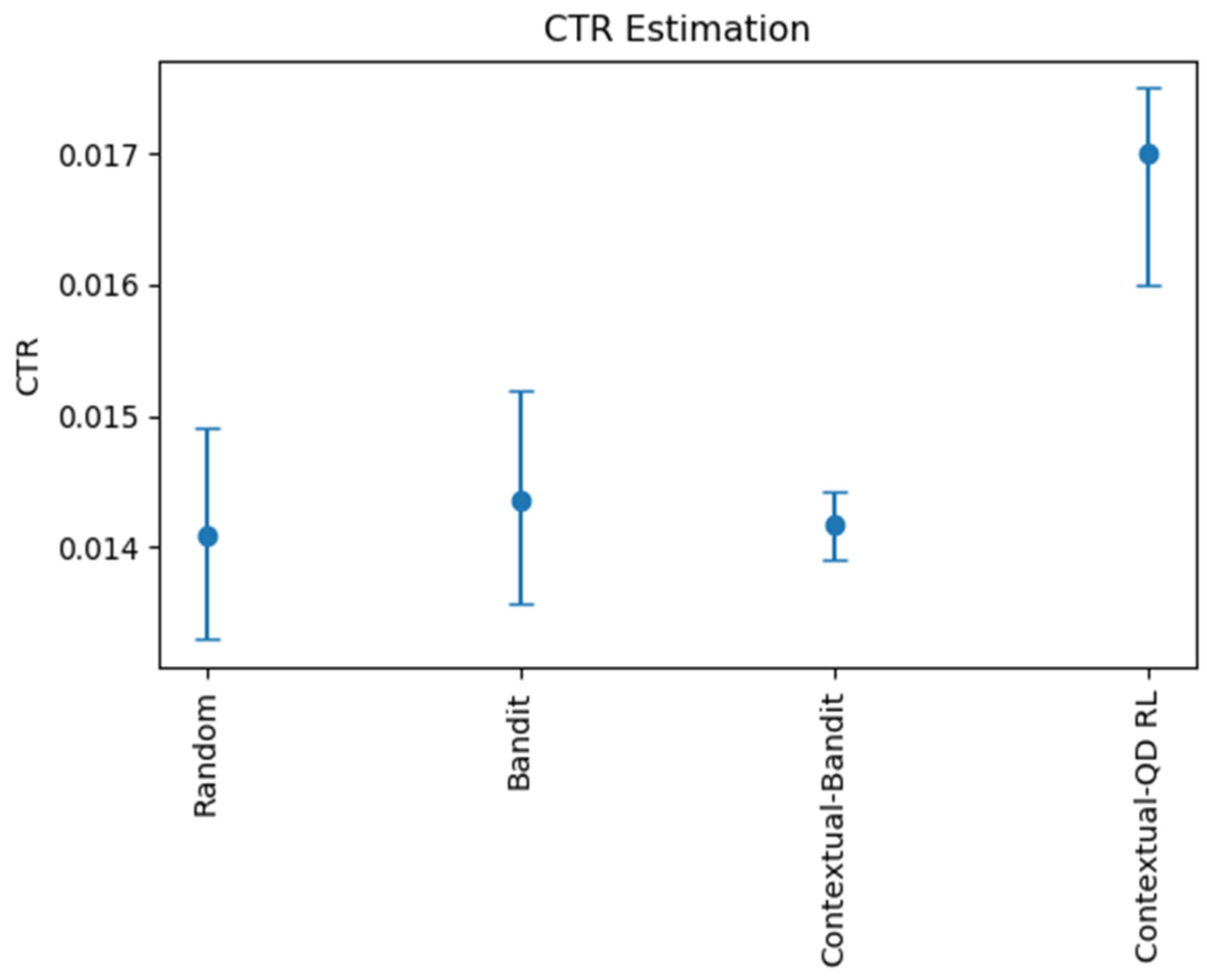
The same experimental logic was used to test the model by using interactive data. The purpose of this experiment was to verify that the enhancement of the contextual–quantile regression reinforcement learning model was effective. Logical regression and bandit, as well as a contextual bandit and the random recommendation algorithm, were used for this experiment. Each algorithm required different parameters; therefore, the parameters of each algorithm were the approximate optimal parameters obtained by conducting a random search. Because the statistical caliber of the interactive data was different from that of the static data, no mutual comparison was made with the static data. The results are shown in Figure 6.

Few differences existed between the bandit model and random recommendation because many goods were involved and the pure interactive data were too sparse for goods to be recommended. Moreover, the bandit model does not consider context. Regarding the context-based reinforcement learning model, its effect was far stronger than the first two because it introduced the information contained in the context. However, because the bandit algorithm is linear, it can still be enhanced. Compared with the other models, the contextual–quantile regression reinforcement learning model was more accurate because it fit more nonlinear information, and the data buffer could alleviate the sparse data problem. From the results, we concluded that the enhancement of the contextual–quantile regression reinforcement learning model was stronger than that of the traditional reinforcement learning method.

5. Conclusions

To introduce nonlinear expectations into the research, design, and practical discussions of reinforcement learning algorithms, we enhanced the way that the recommendation system utilizes data, introduced the value distribution reinforcement learning method, integrated the relevant theories and ideas surrounding nonlinear expectations into the applications of recommendation algorithms, and proposed a fuzzy Mahalanobis metric clustering and sublinear coding enhancement model to accurately describe the characteristics of the users. The contextual–quantile regression reinforcement learning model was proposed to design and verify an algorithm model based on the user’s static characteristics and interactive data and to explain the progressiveness and rationality of the algorithm model based on nonlinear expectations in theory. In addition, because the experiments on and training of the algorithm model occur in environments that are different from the traditional recommendation system environment, we used the collaborative interactive recommender to replace the original core recommendation algorithm model. We found that when combining the model with the data and user characteristics of the e-commerce simulation environment, when modeling fresh data, a personalized recommendation was provided and important indicators such as the CTR were remarkably enhanced; that is, a recommendation algorithm with a nonlinear expectation that could balance various factors and meet the needs of users to the maximum extent was used.

The data utilization, robustness, convergence speed, and stability of the model were greatly increased, which provided theoretical support and an algorithmic basis to provide high-quality recommendation services to users, and the model also has many application prospects. However, the feature engineering method that we used integrates nonlinear expectations into feature engineering. Too many parameters need to be adjusted, and they need to be adjusted according to the actual design and deployment scheme. In the future, more automatic auxiliary parameter adjustment modules can be designed to help optimize the system. At present, though, the model facilitates the rapid transplantation of different data sources and makes them more widely applicable. Finally, because of their high synthesis and complexity, recommendation systems often have features that intersect and fuse with each other. In the face of multimodality, the current contextual–quantile regression reinforcement learning model cannot flexibly adapt to multimodality, and this limitation is worthy of more research.

References

1. Karacan, H.; Karacan, H.; Yenice, Y.E.; Yenice, Y.E.; Al-Sabaawi, A.; Al-Sabaawi, A. A novel overlapping method to alleviate the cold-start problem in recommendation systems. Int. J. Softw. Eng. Knowl. Eng. 2021, 31, 1277–1297. [Google Scholar]
2. Baerg, L.; Bruchmann, K. COVID-19 information overload: Intolerance of uncertainty moderates the relationship between frequency of internet searching and fear of COVID-19. Acta Psychol. 2022, 224, 103534. [Google Scholar] [CrossRef] [PubMed]
3. Ge, M.; Persia, F. A Survey of Multimedia Recommender Systems: Challenges and Opportunities. Int. J. Semant. Comput. 2017, 11, 411–428. [Google Scholar] [CrossRef]
4. Gomez-Uribe, C.A.; Hunt, N. The netflix recommender system. ACM Trans. Manag. Inf. Syst. 2015, 6, 1–19. [Google Scholar] [CrossRef] [Green Version]
5. Zhou, R.; Khemmarat, S.; Gao, L.; Jian, W.; Zhang, J. How youtube videos are discovered and its impact on video views. Multimed. Tools Appl. 2016, 75, 6035–6058. [Google Scholar] [CrossRef]
6. Zhou, R.; Khemmarat, S.; Gao, L. The impact of YouTube recommendation system on video views. In Proceedings of the 10th ACM SIGCOMM Conference on Internet Measurement, Melbourne, Australia, 1–3 November 2010. [Google Scholar]
7. Ikram, F.; Farooq, H. Multimedia recommendation system for video game based on high-level visual semantic features. Sci. Program. 2022, 2022, 6084363. [Google Scholar] [CrossRef]
8. Kiruthika, N.S.; Thailambal, G. Dynamic light weight recommendation system for social networking analysis using a hybrid lstm-svm classifier algorithm. Opt. Mem. Neural Netw. 2022, 31, 59–75. [Google Scholar] [CrossRef]
9. Goldberg, D.; Nichols, D.; Oki, B.M.; Terry, D. Using collaborative filtering to weave an information tapestry. ACM 1992, 35, 61–70. [Google Scholar] [CrossRef]
10. Resnick, P.; Iacovou, N.; Suchak, M.; Bergstrom, P.; Riedl, J. Gruoplens: An open architecture for collaborative filtering of netnews. In Proceedings of the ACM 1994 Conference on Computer Supported Cooperative Work, Chapel Hill, NC, USA, 22–26 October 1994; pp. 175–186. [Google Scholar]
11. Linden, G.; Smith, B.; York, J. Amazon. com recommendations: Item-to-item collaborative filtering. IEEE Internet Comput. 2003, 7, 76–80. [Google Scholar] [CrossRef] [Green Version]
12. Breese, J.S.; Heckerman, D.E.; Kadie, C.M. Empirical analysis of predictive algorithms for collaborative filtering. Uncertain. Artif. Intell. 1998, 98052, 43–52. [Google Scholar]
13. Pazzani, M.J. A framework for collaborative, content-based and demographic filtering. Artif. Intell. Rev. 1999, 13, 393–408. [Google Scholar] [CrossRef]
14. Zhang, S.; Yao, L.; Sun, A.; Tay, Y. Deep learning based recommender system. ACM Comput. Surv. (CSUR) 2019, 52, 1–38. [Google Scholar] [CrossRef] [Green Version]
15. He, X.; Liao, L.; Zhang, H.; Nie, L.; Chua, T.S. Neural collaborative filtering. In Proceedings of the International World Wide Web Conferences Steering Committee, Perth, Australia, 3–7 April 2017; pp. 173–182. [Google Scholar]
16. Hidasi, B.; Karatzoglou, A.; Baltrunas, L.; Tikk, D. Session-based recommendations with recurrent neural networks. In Proceedings of the 4th International Conference on Learning Representations, San Juan, Puerto Rico, 2–4 May 2016; pp. 498–506. [Google Scholar]
17. Pang, J.; Hegde, V.; Chalupsky, J. Upper Confidence Bound Algorithm for Oilfield Logic. U.S. Patent US20210150440A1, 20 May 2021. [Google Scholar]
18. Prashanth, L.A.; Korda, N.; Munos, R. Concentration bounds for temporal difference learning with linear function approximation: The case of batch data and uniform sampling. Mach. Learn. 2021, 110, 559–618. [Google Scholar] [CrossRef]
19. Seminario, C.E.; Wilson, D.C. Nuke Em Till They Go: Investigating Power User Attacks to Disparage Items in Collaborative Recommenders. In Proceedings of the 9th ACM Conference on Recommender Systems, Vienna, Austria, 16–20 September 2015; pp. 293–296. [Google Scholar]
20. Dornheim, J.; Link, N.; Gumbsch, P. Model-free adaptive optimal control of episodic fixed-horizon manufacturing processes using reinforcement learning. Int. J. Control Autom. Syst. 2020, 18, 1593–1604. [Google Scholar] [CrossRef] [Green Version]
21. Jwk, A.; Bjp, A.; Hy, B.; Tho, A.; Jhl, B.; Jml, A. A model-based deep reinforcement learning method applied to finite-horizon optimal control of nonlinear control-affine system. J. Process Control 2020, 87, 166–178. [Google Scholar]
22. Ie, E.; Jain, V.; Wang, J.; Narvekar, S.; Boutilier, C. SlateQ: A Tractable Decomposition for Reinforcement Learning with Recommendation Sets. In Proceedings of the Twenty-Eighth International Joint Conference on Artificial Intelligence, Macao, China, 10–16 August 2019; pp. 2592–2599. [Google Scholar]
23. Shani, G.; Heckerman, D.; Brafman, R.I.; Boutilier, C. An mdp-based recommender system. J. Mach. Learn. Res. 2005, 6, 1265–1295. [Google Scholar]
24. Zhao, X.; Xia, L.; Zhang, L.; Ding, Z.; Yin, D.; Tang, J. Deep reinforcement learning for page-wise recommendations. In Proceedings of the 12th ACM Conference on Recommender Systems, Vancouver, BC, Canada, 2 October 2018; pp. 95–103. [Google Scholar]
25. Christakopoulou, K.; Banerjee, A. Learning to Interact with Users: A Collaborative-Bandit Approach. In Proceedings of the 2018 SIAM International Conference on Data Mining, San Diego, CA, USA, 3–5 May 2018; pp. 612–620. [Google Scholar]
26. Li, S.; Karatzoglou, A.; Gentile, C. Collaborative Filtering Bandits. In Proceedings of the 39th International ACM SIGIR Conference on Research and Development in Information Retrieval, Pisa, Italy, 17–21 July 2016; pp. 539–548. [Google Scholar]
27. Vinyals, O.; Le, Q. A neural conversational model. Computer Science. In Proceedings of the ICML Deep Learning Workshop, Lille, France, 6–11 July 2015. [Google Scholar]
28. Candès, E.J.; Tao, T. The power of convex relaxation: Near-optimal matrix completion. IEEE Trans. Inf. Theory 2010, 56, 2053–2080. [Google Scholar] [CrossRef] [Green Version]
29. Mcnee, S.M.; Riedl, J.; Konstan, J.A. Being accurate is not enough: How accuracy metrics have hurt recommender systems. In Proceedings of the Extended Abstracts 2006 Conference on Human Factors in Computing Systems, Montréal, QC, Canada, 22–27 April 2006; pp. 1097–1101. [Google Scholar]
30. Hz, A.; Cp, B.; Bm, A.; Tl, A.; Hv, A. New technique to alleviate the cold start problem in recommender systems using information from social media and random decision forests—Sciencedirect. Inf. Sci. 2020, 536, 156–170. [Google Scholar]
31. Liu, K.; Wei, L.; Chen, X. A new preference-based model to solve the cold start problem in a recommender system. In Proceedings of the 2nd International Conference on Electromechanical Control Technology and Transportation, Zhuhai, China, 14–15 January 2017; pp. 121–126. [Google Scholar]
32. Kvr, A.; Sjm, B.; Tb, C. Model-Driven Approach Running Route two-level SVD with Context Information and Feature Entities in Recommender System. Comput. Stand. Interfaces 2022, 82, 103627. [Google Scholar]
33. Xu, R.; Li, J.; Li, G.; Pan, P.; Zhou, Q.; Wang, C. Sdnn: Symmetric deep neural networks with lateral connections for recommender systems. Inf. Sci. 2022, 595, 217–230. [Google Scholar] [CrossRef]
Figure 1. Markov process of user browsing session and interactive session.
Mathematics 11 02895 g001
Figure 2. Segment statistics of user interaction.
Mathematics 11 02895 g002
Figure 3. Violin chart of exploration click-through rate indicators of different users.
Mathematics 11 02895 g003
Figure 4. HR@5 comparison chart of various static characteristic engineering methods.
Mathematics 11 02895 g004
Figure 5. CTR comparison chart of various static characteristic engineering methods.
Mathematics 11 02895 g005
Figure 6. Model comparison of interactive data.
Mathematics 11 02895 g006