


Adaptive Super-Twisting Sliding Mode Control of Active Power Filter Using Interval Type-2-Fuzzy Neural Networks


Abstract
:1. Introduction
- (1)
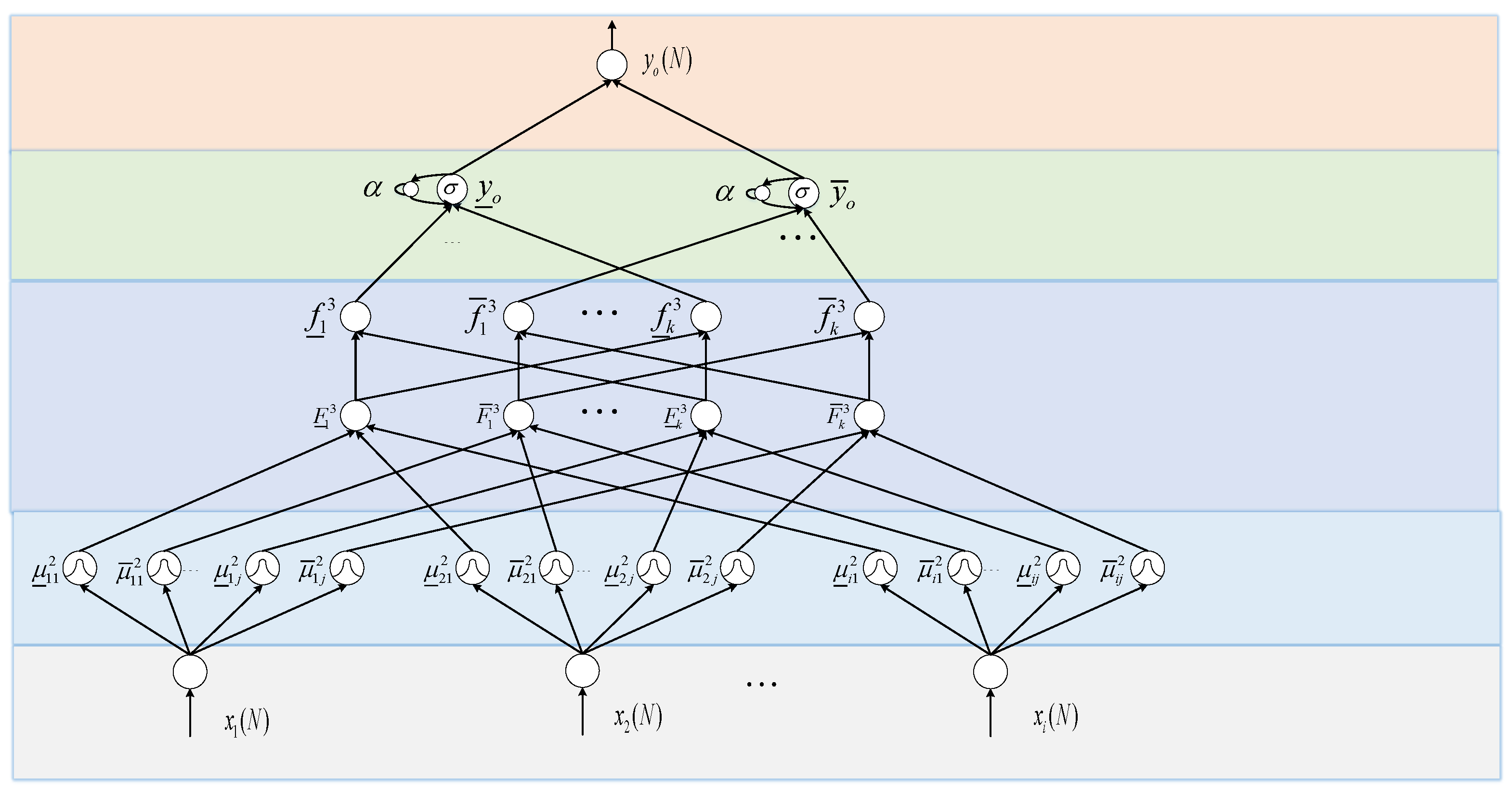
- A new structure of IT2FNN, namely IT2FNN-SFR, has been proposed, which has the ability of strong robustness as IT2FNN and great dynamic response as RNN. The new NN is error-driven and online optimization, which means it is less dependent on accurate and detailed information about the system. The recursive structure in the NN will store and take advantage of the historical information to improve the accuracy of estimation and dynamic approximation effect;
- (2)
- STSMC not only has the advantages of strong robustness and simple control principle of traditional SMC but also overcomes the chattering problem. In order to reduce the inaccuracy and complexity of manual parameter setting, a sliding mode gain adaptive law is deduced to realize a set of gain optimal solutions.
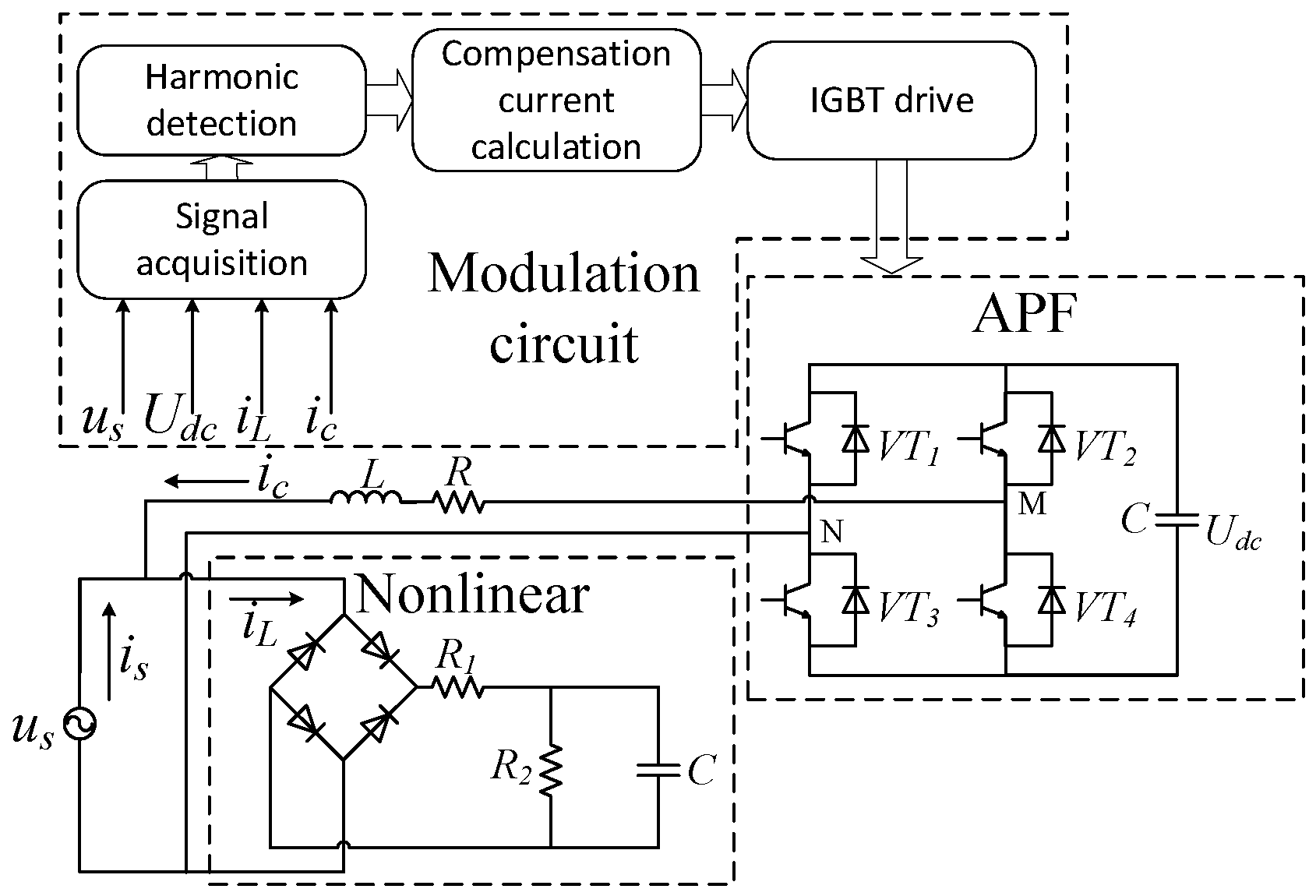
2. Principle of Active Power Filter
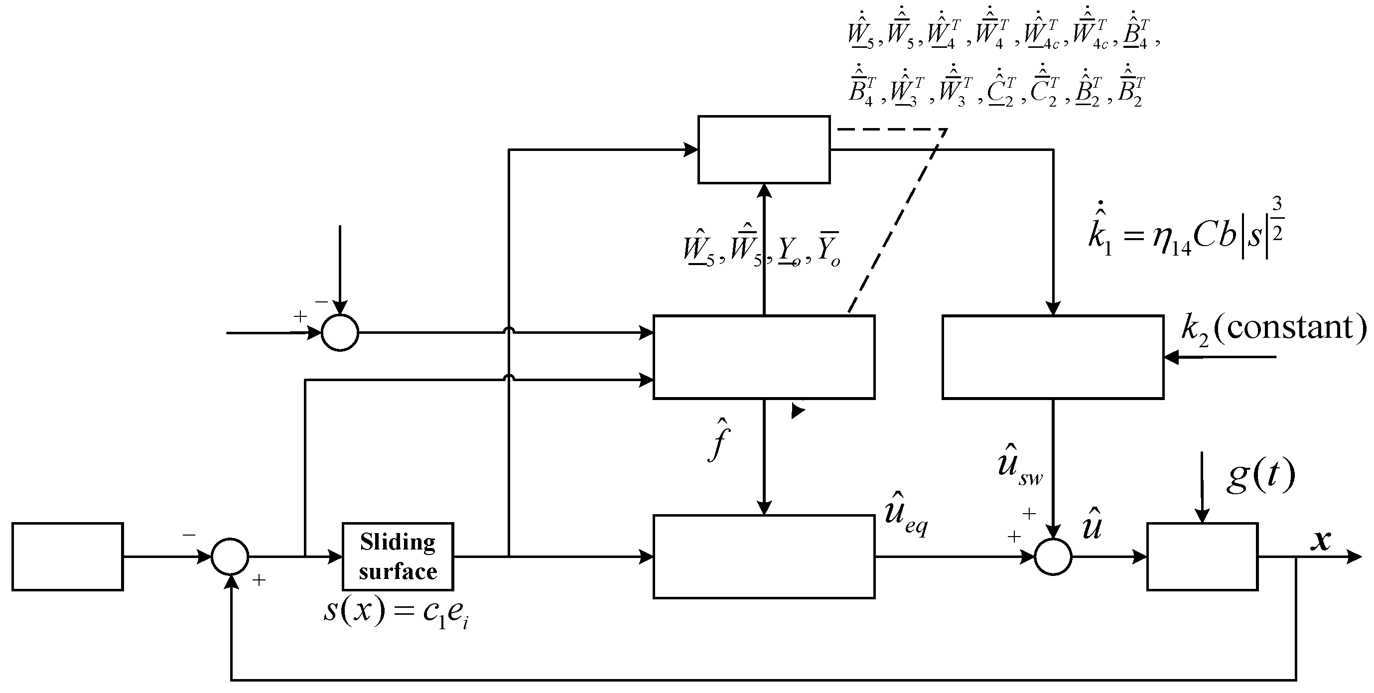
3. Controller Design and Analysis
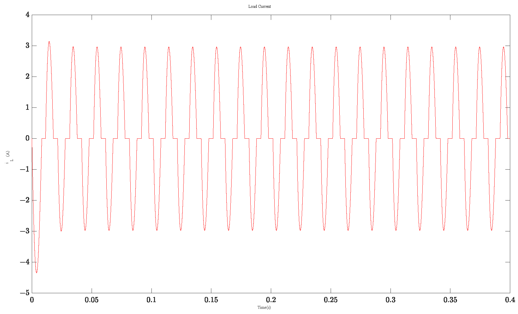
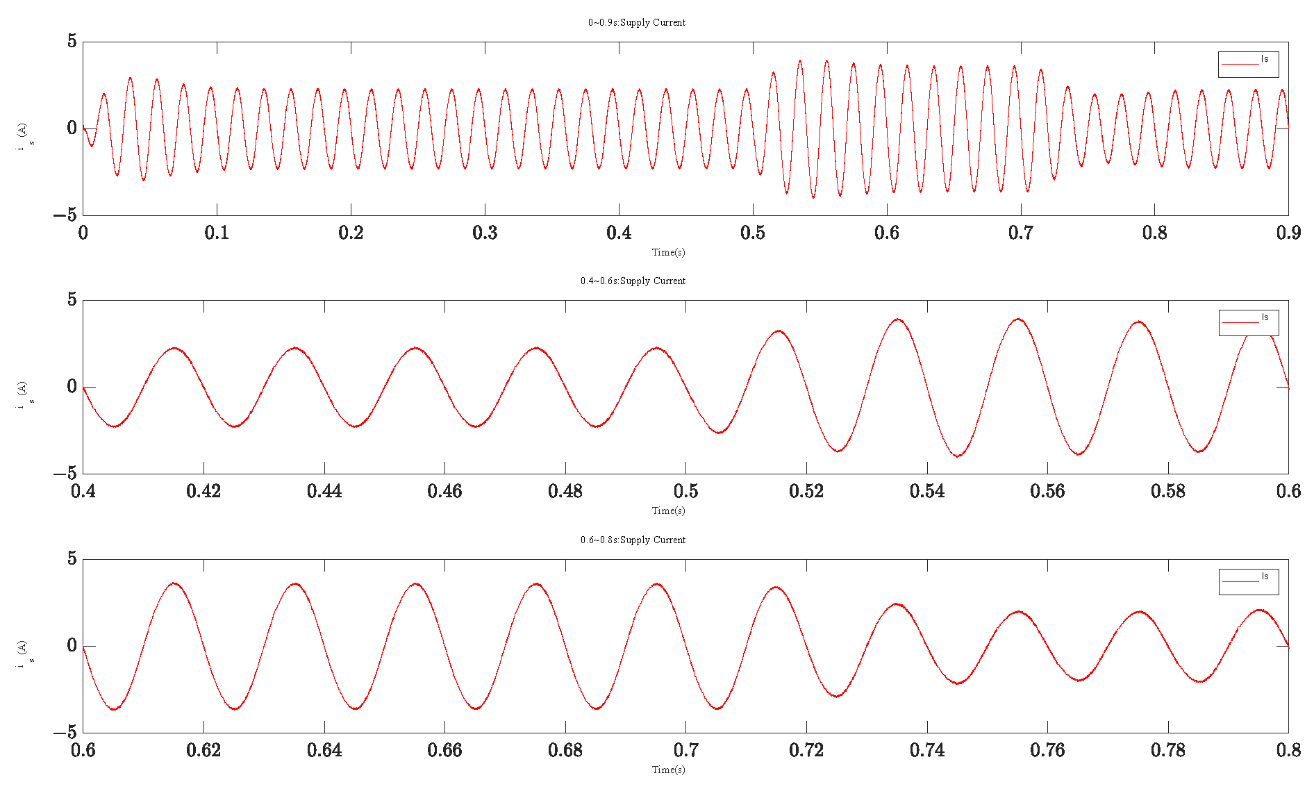
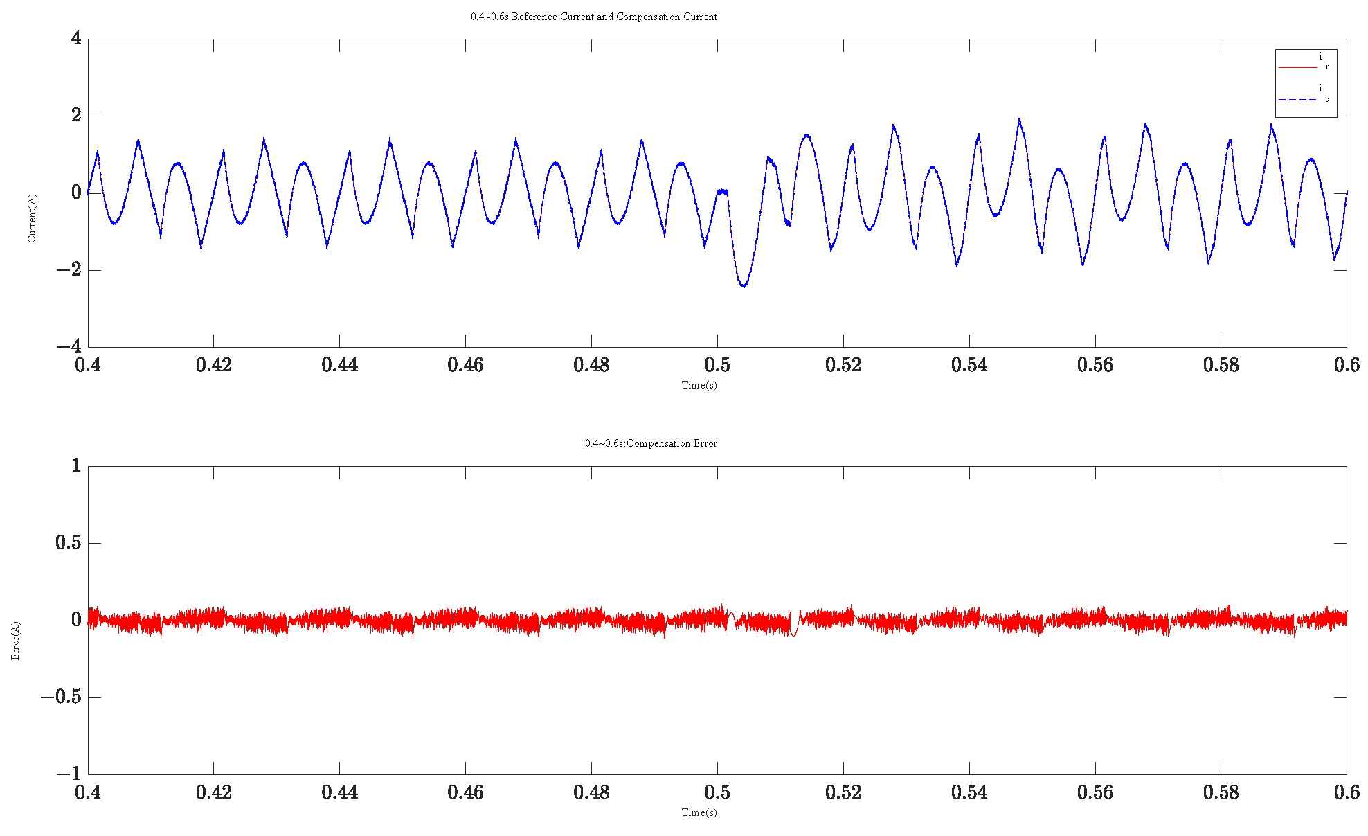
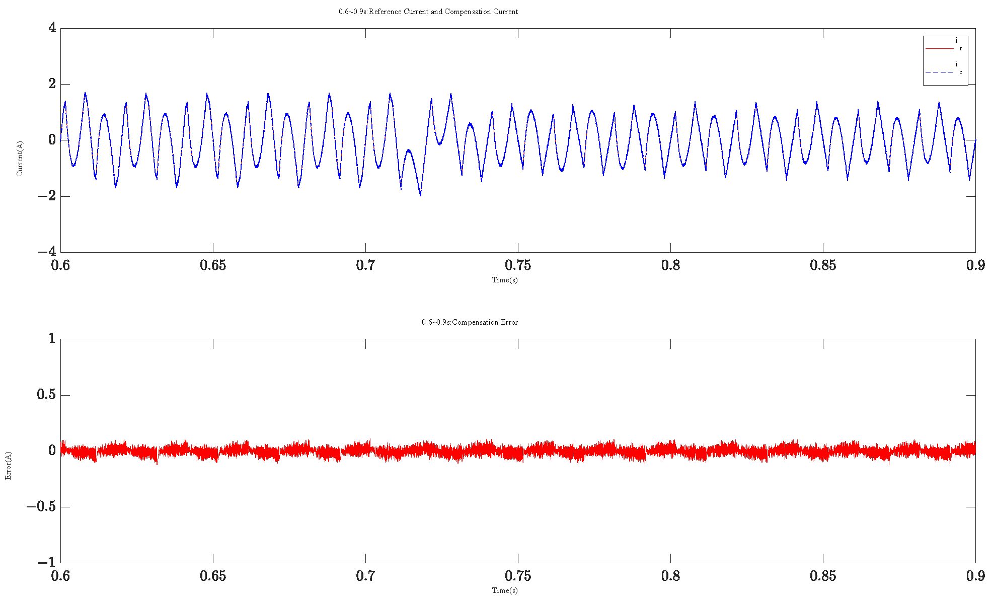
4. Numerical Verification
5. Conclusions
Author Contributions
Funding
Data Availability Statement
Conflicts of Interest
References
- Wu, Z.; Yang, Z.; Ding, K.; He, G. Order-Domain-Based Harmonic Injection Method for Multiple Speed Harmonics Suppression of PMSM. IEEE Trans. Power Electron. 2021, 36, 4478–4487. [Google Scholar] [CrossRef]
- RGregory, R.; Azevedo, C.; Santos, I. Study of Harmonic Distortion Propagation from a Wind Park. IEEE Lat. Am. Trans. 2020, 18, 1077–1084. [Google Scholar] [CrossRef]
- Jiao, N.; Wang, S.; Ma, J.; Chen, X.; Liu, T.; Zhou, D.; Yang, Y. The Closed-Loop Sideband Harmonic Suppression for CHB Inverter with Unbalanced Operation. IEEE Trans. Power Electron. 2022, 37, 5333–5341. [Google Scholar] [CrossRef]
- Fu, J.; Chen, L.; Zhao, H.; Zhang, P. High and Low Frequency Control Strategy for APF DC Side Ripple Voltage under Unbalanced Load. In Proceedings of the 2019 IEEE 2nd International Conference on Electronics and Communication Engineering (ICECE), Xi’an, China, 9–11 December 2019; pp. 326–330. [Google Scholar]
- Vahedi, H.; Shojaei, A.A.; Dessaint, L.-A.; Al-Haddad, K. Reduced DC-Link Voltage Active Power Filter Using Modified PUC5 Converter. IEEE Trans. Power Electron. 2018, 33, 943–947. [Google Scholar] [CrossRef]
- Incremona, G.P.; Rubagotti, M.; Ferrara, A. Sliding Mode Control of Constrained Nonlinear Systems. IEEE Trans. Autom. Control 2017, 62, 2965–2972. [Google Scholar] [CrossRef] [Green Version]
- Hou, L.; Ma, J.; Wang, W. Sliding Mode Predictive Current Control of Permanent Magnet Synchronous Motor with Cascaded Variable Rate Sliding Mode Speed Controller. IEEE Access 2022, 10, 33992–34002. [Google Scholar] [CrossRef]
- Qu, L.; Qiao, W.; Qu, L. An Extended-State-Observer-Based Sliding-Mode Speed Control for Permanent-Magnet Synchronous Motors. IEEE J. Emerg. Sel. Top. Power Electron. 2021, 9, 1605–1613. [Google Scholar] [CrossRef]
- Chen, X.; Li, Y.; Ma, H.; Tang, H.; Xie, Y. A Novel Variable Exponential Discrete Time Sliding Mode Reaching Law. IEEE Trans. Circuits Syst. II Express Briefs 2021, 68, 2518–2522. [Google Scholar] [CrossRef]
- Liu, H.; Wang, H.; Sun, J. Attitude control for QTR using exponential nonsingular terminal sliding mode control. J. Syst. Eng. Electron. 2019, 30, 191–200. [Google Scholar]
- Ren, L.; Lin, G.; Zhao, Y.; Liao, Z.; Peng, F. Adaptive Nonsingular Finite-Time Terminal Sliding Mode Control for Synchronous Reluctance Motor. IEEE Access 2021, 9, 51283–51293. [Google Scholar] [CrossRef]
- Fei, J.; Wang, H.; Fang, Y. Novel Neural Network Fractional-Order Sliding-Mode Control with Application to Active Power Filter. IEEE Trans. Syst. Man Cybern. Syst. 2022, 52, 3508–3518. [Google Scholar] [CrossRef]
- Bo, L.; Peng, J.; Chong, K.T.; Rodriguez, J.; Guerrero, J.M. Robust Fuzzy-Fractional-Order Nonsingular Terminal Sliding-Mode Control of LCL-Type Grid-Connected Converters. IEEE Trans. Ind. Electron. 2022, 69, 5854–5866. [Google Scholar]
- Liu, Y.-J.; Chen, H. Adaptive Sliding Mode Control for Uncertain Active Suspension Systems with Prescribed Performance. IEEE Trans. Syst. Man Cybern. Syst. 2021, 51, 6414–6422. [Google Scholar] [CrossRef]
- Roy, S.; Roy, S.B.; Lee, J.; Baldi, S. Overcoming the Underestimation and Overestimation Problems in Adaptive Sliding Mode Control. IEEE/ASME Trans. Mechatron. 2019, 24, 2031–2039. [Google Scholar] [CrossRef] [Green Version]
- Roy, S.; Baldi, S.; Fridman, L.M. On adaptive sliding mode control without a priori bounded uncertainty. Automatica 2020, 111, 108650. [Google Scholar] [CrossRef]
- Levant, A. Higher-order sliding modes, differentiation and output-feedback control. Int. J. Control. 2003, 76, 924–941. [Google Scholar] [CrossRef]
- Guo, J. The Load Frequency Control by Adaptive High Order Sliding Mode Control Strategy. IEEE Access 2022, 10, 25392–25399. [Google Scholar] [CrossRef]
- Shah, I.; Rehman, F.U. Smooth Second Order Sliding Mode Control of a Class of Underactuated Mechanical Systems. IEEE Access 2018, 6, 7759–7771. [Google Scholar] [CrossRef]
- Chalanga, A.; Kamal, S.; Fridman, L.M.; Bandyopadhyay, B.; Moreno, J.A. Implementation of Super-Twisting Control: Super-Twisting and Higher Order Sliding-Mode Observer-Based Approaches. IEEE Trans. Ind. Electron. 2016, 63, 3677–3685. [Google Scholar] [CrossRef]
- Wu, Y.; Ma, F.; Liu, X.; Hua, Y.; Liu, X.; Li, G. Super Twisting Disturbance Observer-Based Fixed-Time Sliding Mode Backstepping Control for Air-Breathing Hypersonic Vehicle. IEEE Access 2021, 8, 17567–17583. [Google Scholar] [CrossRef]
- Wang, W.; Ma, J.; Li, X.; Cheng, Z.; Zhu, H.; Teo, C.S.; Lee, T.H. Iterative Super-Twisting Sliding Mode Control for Tray Indexing System with Unknown Dynamics. IEEE Trans. Ind. Electron. 2020, 68, 9855–9865. [Google Scholar] [CrossRef]
- Merayo, N.; Juárez, D.; Aguado, J.C.; de Miguel, I.; Durán, R.J.; Fernández, P.; Lorenzo, R.M.; Abril, E.J. PID Controller Based on a Self-Adaptive Neural Network to Ensure QoS Bandwidth Requirements in Passive Optical Networks. J. Opt. Commun. Netw. 2017, 9, 433–445. [Google Scholar] [CrossRef] [Green Version]
- Dai, W.; Zhang, L.; Fu, J.; Chai, T.; Ma, X. Dual-Rate Adaptive Optimal Tracking Control for Dense Medium Separation Process Using Neural Networks. IEEE Trans. Neural Netw. Learn. Syst. 2021, 32, 4202–4216. [Google Scholar] [CrossRef]
- Yang, Y.; Ye, Y. Backstepping sliding mode control for uncertain strict-feedback nonlinear systems using neural-network-based adaptive gain scheduling. J. Syst. Eng. Electron. 2018, 29, 580–586. [Google Scholar]
- Li, K.; Li, Y. Adaptive Neural Network Finite-Time Dynamic Surface Control for Nonlinear Systems. IEEE Trans. Neural Netw. Learn. Syst. 2021, 32, 5688–5697. [Google Scholar] [CrossRef]
- Liu, X.; Su, C.-Y.; Yang, F. FNN Approximation-Based Active Dynamic Surface Control for Suppressing Chatter in Micro-Milling with Piezo-Actuators. IEEE Trans. Syst. Man Cybern. Syst. 2017, 47, 2100–2113. [Google Scholar] [CrossRef]
- Wai, R.; Yao, J.; Lee, J. Backstepping Fuzzy-Neural-Network Control Design for Hybrid Maglev Transportation System. IEEE Trans. Neural Netw. Learn. Syst. 2015, 26, 302–317. [Google Scholar] [PubMed]
- Wai, R.-J.; Chen, M.-W.; Liu, Y.-K. Design of Adaptive Control and Fuzzy Neural Network Control for Single-Stage Boost Inverter. IEEE Trans. Ind. Electron. 2015, 62, 5434–5445. [Google Scholar] [CrossRef]
- Liu, L.; Fei, J. Extended State Observer Based Interval Type-2 Fuzzy Neural Network Sliding Mode Control with Its Application in Active Power Filter. IEEE Trans. Power Electron. 2022, 37, 5138–5154. [Google Scholar] [CrossRef]
- Wang, J.; Luo, W.; Liu, J.; Wu, L. Adaptive Type-2 FNN-Based Dynamic Sliding Mode Control of DC–DC Boost Converters. IEEE Trans. Syst. Man, Cybern. Syst. 2021, 51, 2246–2257. [Google Scholar] [CrossRef]
- Gao, Y.; Liu, J.; Wang, Z.; Wu, L. Interval Type-2 FNN-Based Quantized Tracking Control for Hypersonic Flight Vehicles with Prescribed Performance. IEEE Trans. Syst. Man Cybern. Syst. 2021, 51, 1981–1993. [Google Scholar] [CrossRef]
- Kim, C.-J.; Chwa, D. Obstacle Avoidance Method for Wheeled Mobile Robots Using Interval Type-2 Fuzzy Neural Network. IEEE Trans. Fuzzy Syst. 2015, 23, 677–687. [Google Scholar] [CrossRef]
- Wai, R.-J.; Lin, C.-M.; Peng, Y.-F. Adaptive Hybrid Control for Linear Piezoelectric Ceramic Motor Drive Using Diagonal Recurrent CMAC Network. IEEE Trans. Neural Netw. 2004, 15, 1491–1506. [Google Scholar] [CrossRef] [PubMed]
- Yogi, S.C.; Tripathi, V.K.; Behera, L. Adaptive Integral Sliding Mode Control Using Fully Connected Recurrent Neural Network for Position and Attitude Control of Quadrotor. IEEE Trans. Neural Netw. Learn. Syst. 2021, 32, 5595–5609. [Google Scholar] [CrossRef]
- Fei, J.; Chen, Y.; Liu, L.; Fang, Y. Fuzzy Multiple Hidden Layer Recurrent Neural Control of Nonlinear System Using Terminal Sliding-Mode Controller. IEEE Trans. Cybern. 2022, 52, 9519–9534. [Google Scholar] [CrossRef]
- Fei, J.; Liu, L. Real-Time Nonlinear Model Predictive Control of Active Power Filter Using Self-Feedback Recurrent Fuzzy Neural Network Estimator. IEEE Trans. Ind. Electron. 2022, 69, 8366–8376. [Google Scholar] [CrossRef]
- Han, H.-G.; Zhang, L.; Hou, Y.; Qiao, J.-F. Nonlinear Model Predictive Control Based on a Self-Organizing Recurrent Neural Network. IEEE Trans. Neural Networks Learn. Syst. 2016, 27, 402–415. [Google Scholar] [CrossRef]
- Fei, J.; Wang, Z.; Pan, Q. Self-Constructing Fuzzy Neural Fractional-Order Sliding Mode Control of Active Power Filter. IEEE Trans. Neural Networks Learn. Syst. 2022. [Google Scholar] [CrossRef]
- Fei, J.; Wang, Z.; Fang, Y. Self-Evolving Chebyshev Fuzzy Neural Fractional-Order Sliding Mode Control for Active Power Filter. IEEE Trans. Ind. Inform. 2022, 19, 2729–2739. [Google Scholar] [CrossRef]
- Wang, J.; Fei, J. Self-Feedback Neural Network Sliding Mode Control with Extended State Observer for Active Power Filter. IEEE Internet Things J. 2023. [Google Scholar] [CrossRef]
- Zhang, L.; Fei, J. Intelligent Complementary Terminal Sliding Mode Using Multi-Loop Neural Network for Active Power Filter. IEEE Trans. Power Electron. 2023. [Google Scholar] [CrossRef]


| Strategy | ASMC | FNNASMC-SFR based on LESO [41] | IT2FNN-SFR STSMC | CTSMC-MLNN [42] |
|---|---|---|---|---|
| Time(s) | 5.5619 | 15.795 | 28.234 | 32.829 |
| Parameters | Values |
|---|---|
| Supply voltage | |
| APF main circuit | , , , |
| Non-linear load at steady state | , |
| Additional non-linear load in parallel | , |
| Sampling time |
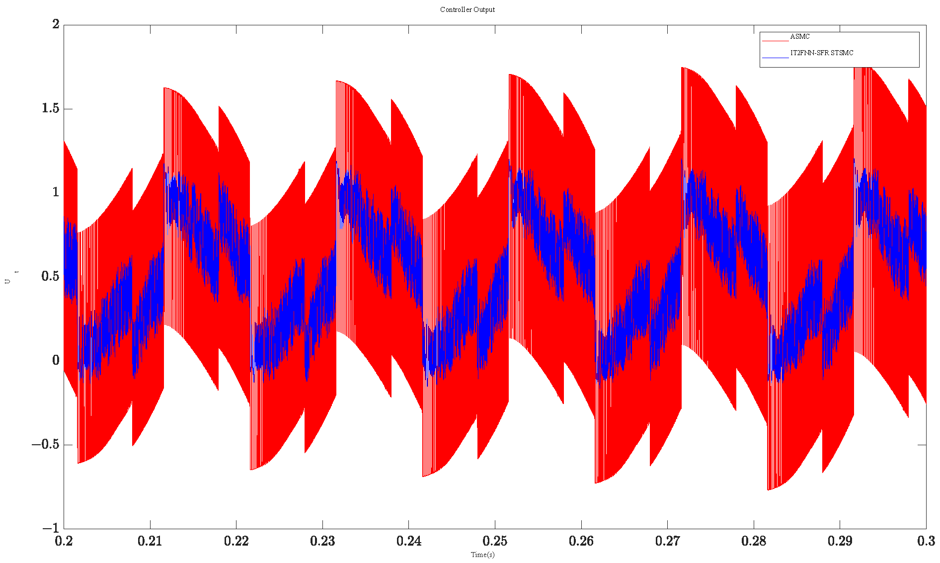
| Strategy Index | IT2FNN-SFR STSMC | ASMC |
|---|---|---|
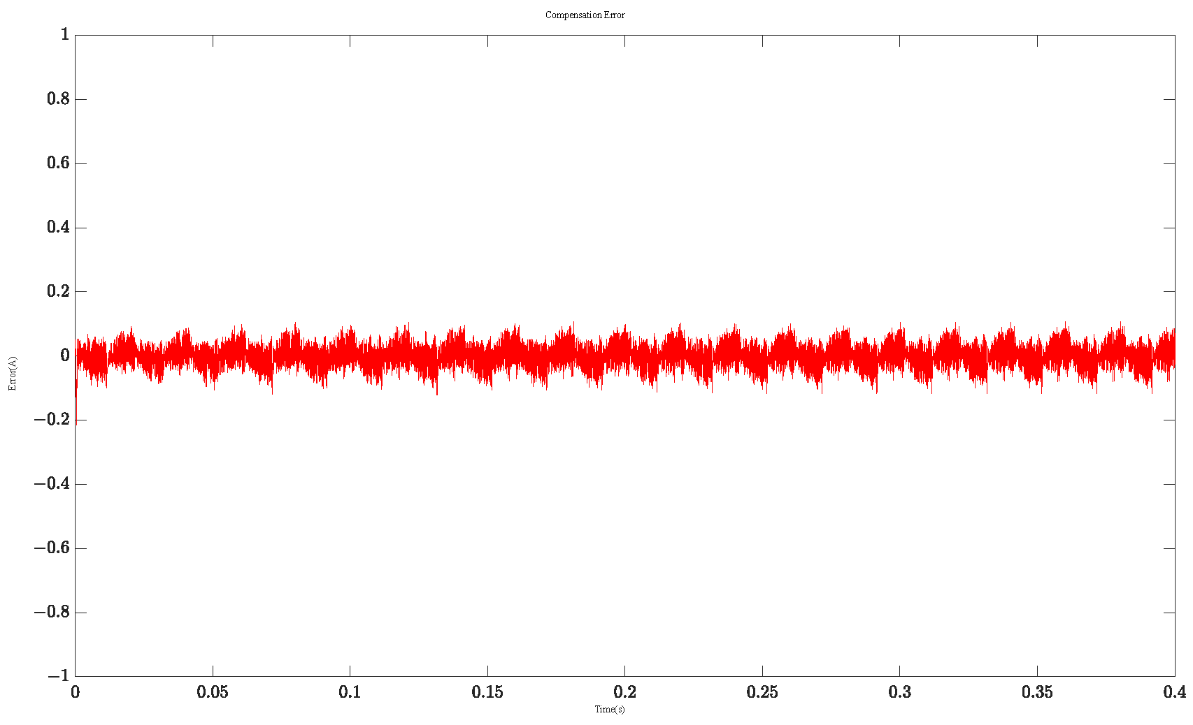
| Output variance | 0.0650 | 0.1362 |
| Control Strategy | 0 s | 0.2 s | 0.6 s | 0.8 s |
|---|---|---|---|---|
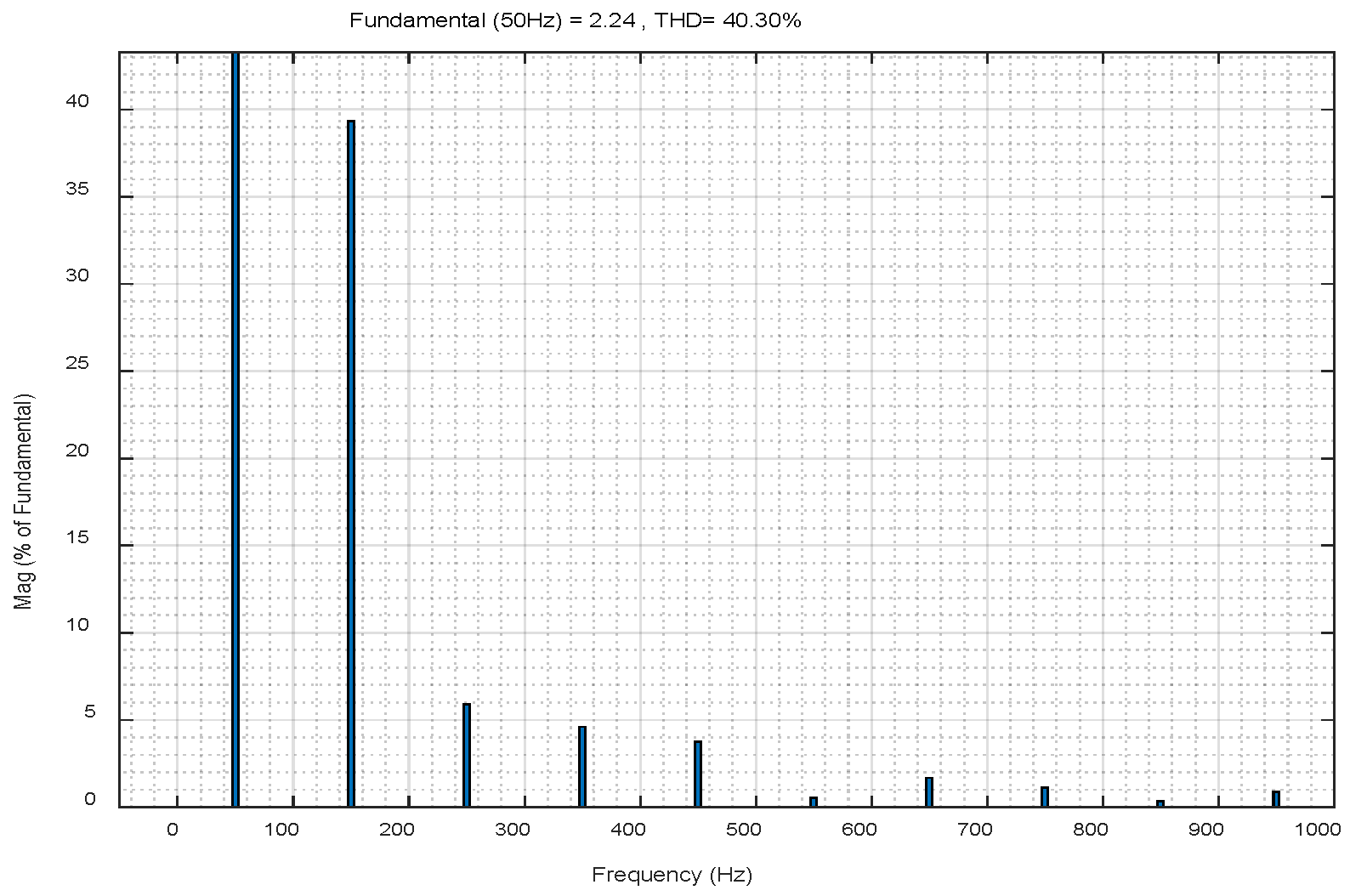
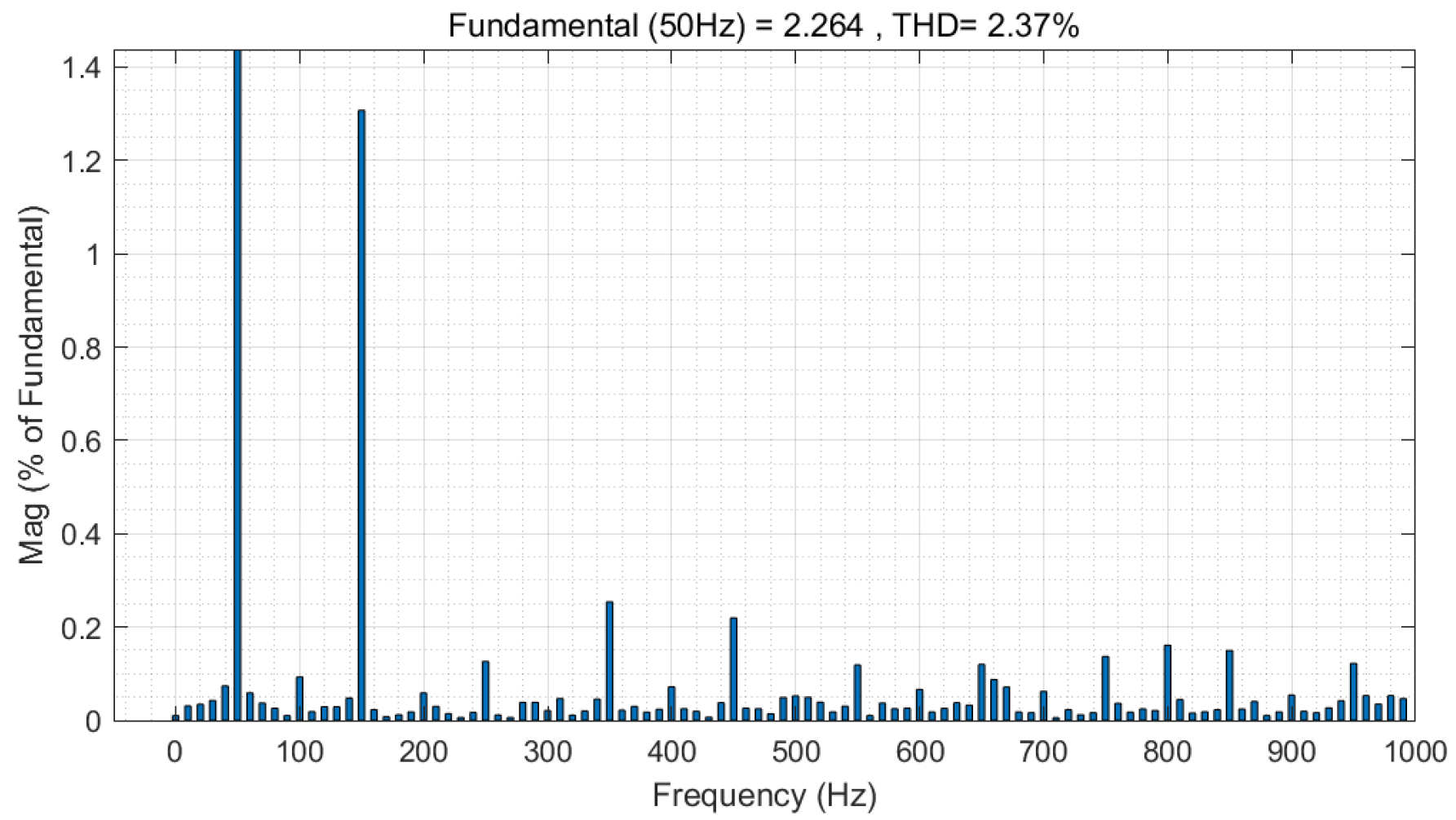
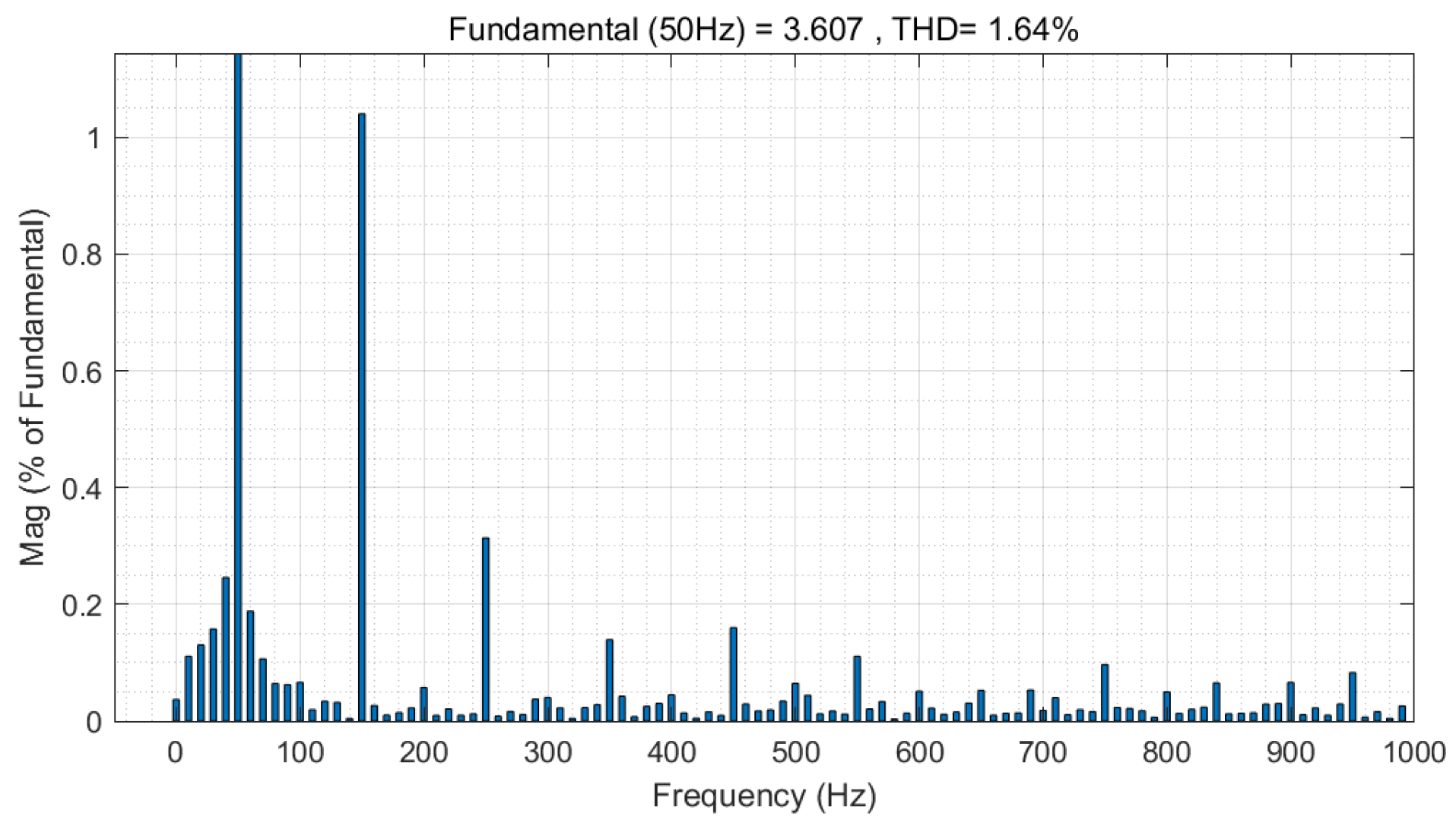
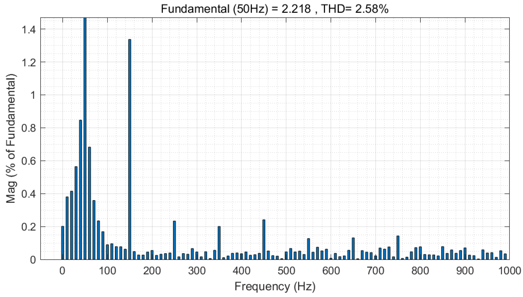
| IT2FNN-SFR STSMC | 16.44% | 2.37% | 1.64% | 2.58% |
| ASMC | 20.03% | 2.66% | 1.68% | 2.92% |
Disclaimer/Publisher’s Note: The statements, opinions and data contained in all publications are solely those of the individual author(s) and contributor(s) and not of MDPI and/or the editor(s). MDPI and/or the editor(s) disclaim responsibility for any injury to people or property resulting from any ideas, methods, instructions or products referred to in the content. |
© 2023 by the authors. Licensee MDPI, Basel, Switzerland. This article is an open access article distributed under the terms and conditions of the Creative Commons Attribution (CC BY) license (https://creativecommons.org/licenses/by/4.0/).
Share and Cite
Wang, J.; Fang, Y.; Fei, J. Adaptive Super-Twisting Sliding Mode Control of Active Power Filter Using Interval Type-2-Fuzzy Neural Networks. Mathematics 2023, 11, 2785. https://doi.org/10.3390/math11122785
Wang J, Fang Y, Fei J. Adaptive Super-Twisting Sliding Mode Control of Active Power Filter Using Interval Type-2-Fuzzy Neural Networks. Mathematics. 2023; 11(12):2785. https://doi.org/10.3390/math11122785
Chicago/Turabian StyleWang, Jiacheng, Yunmei Fang, and Juntao Fei. 2023. "Adaptive Super-Twisting Sliding Mode Control of Active Power Filter Using Interval Type-2-Fuzzy Neural Networks" Mathematics 11, no. 12: 2785. https://doi.org/10.3390/math11122785