
John von Neumann’s Time-Frequency Orthogonal Transforms


Faculty of Automatic Control and Computers, “Politehnica” University of Bucharest, 313 Splaiul Independentei, 060042 Bucharest, Romania
*
Author to whom correspondence should be addressed.
Mathematics 2023, 11(12), 2607; https://doi.org/10.3390/math11122607
Submission received: 30 April 2023
/
Revised: 1 June 2023
/
Accepted: 2 June 2023
/
Published: 7 June 2023
(This article belongs to the Special Issue Automatic Control and Soft Computing in Engineering)
Abstract
:John von Neumann (JvN) was one of the greatest scientists and minds of the 20th century. His research encompassed a large variety of topics (especially from mathematics), and the results he obtained essentially contributed to the progress of science and technology. Within this article, one function that JvN defined long time ago, namely the cardinal sinus (sinc), was employed to define transforms to be applied on 1D signals, either in continuous or discrete time. The main characteristics of JvN Transforms (JvNTs) are founded on a theory described at length in the article. Two properties are of particular interest: orthogonality and invertibility. Both are important in the context of data compression. After building the theoretical foundation of JvNTs, the corresponding numerical algorithms were designed, implemented and tested on artificial and real signals. The last part of the article is devoted to simulations with such algorithms by using 1D signals. An extensive analysis on JvNTs effectiveness is performed as well, based on simulation results. In conclusion, JvNTs prove to be useful tools in signal processing.
Keywords:
numerable bases in Lebesgue-Hilbert space; orthogonal transforms; time-frequency dictionary; Fourier transforms; analysis and synthesis of finite energy signalsMSC:
47N70; 40B99; 40C99; 40D99; 40E991. Introduction
Orthogonality is an important and interesting, yet challenging, property in pure mathematics, as well as in some branches of applied mathematics (such as system identification [1] or signal processing (SP) [2]). One of the oldest results regarding orthogonality is the ancient Pythagorean theorem, which suggested that some mathematical entity (e.g., the hypotenuse vector) can be expressed by means of other entities, which are orthogonal to each other (e.g., the catheti unit vectors), as a linear combination of them. Moreover, thanks to orthogonality, the coefficients of linear combination are easily computed by simply projecting the mathematical entity on each orthogonal entity. One refers to this operation to as analysis or decomposing. Thus, the mathematical entity can be replaced by the coefficients, provided that the orthogonal entities are known. From coefficients, the mathematical entity can be either partially or fully recovered by using the linear combination. This operation stands for synthesis or recomposing of the mathematical entity. The orthogonal entities put together constitute a so-called transform (Often, the transform is expressed by means of an orthogonal/Hermitian matrix). They also can play the role of bases in a vectorial space. It’s very likely that Pythagoras was not using this terminology, which started to be known much later. However, his idea generated an intense quest for orthogonal transforms or bases and has had a huge impact in modern technology. Since Pythagoras’ times, myriads of orthogonality results have been derived. To reveal the framework of this article, only very few of them are cited next.
The vectorial spaces of interest for this article are the ones defined by Lebesgue, either in continuous or discrete time, for 1D functions, also referred to as signals. (Recall that any signal from a Lebesgue space is -integrable or -summable, which automatically involves the signal’s being bounded). It has been proven that all Lebesgue spaces are of a Banach type, which means that norms yield computing distances between signals. Even more interesting are the spaces for , since the discussion on orthogonality can be extended from time domain to frequency domain () and a scalar product can serve as important tool for testing orthogonality between signals (). (Actually, for , the Lebesgue space also is a Hilbert space).
In pure mathematics, polynomials are comfortable mathematical entities selected to build orthogonal bases. Among them, Chebyshev polynomials [3] are remarkable in this respect. Nowadays, squared Krawtchouk–Chebyshev polynomials are successfully employed in applications [4]. Another interesting development is reported in the context of the Euclidean and Weyl–Heisenberg (uncertainty) groups [5], where Hermite functions are employed. The Weyl–Heisenberg group belongs to the larger class of Lie groups and is particularly interesting, as the analysis is approached not only in the time domain, but also in the frequency domain, by using the two linear operators which are defined within this article as well. Some unconventional orthogonal bases are proposed as well. For example, in [6], the basis is founded on discrete spherical Bessel functions.
One of the most notorious orthogonal bases was introduced by J. Fourier more than 200 years ago and is harmonic in nature. This was an important breakthrough which led not only to the concepts of Fourier series and Fourier transform (FT), but also to the combined time-frequency approach. The Dirichlet-Fourier punctual convergence theorem is a fundamental result [7] for harmonic analysis and synthesis. Nowadays, numerical algorithms of the fast Fourier transform class [2] are employed in various fields. They implement the discrete Fourier transform (DFT) formula in efficient manner. Nowadays, implementations benefit from parallel computing, which has allowed reaching a milestone in terms of speed [8,9]. From this class of procedures, the discrete cosine transform (DCT) algorithm is integrated in many standards of signal compression and coding [10].
Although the FT dominated the research for long time, some other orthogonal transforms were defined, especially in recent decades. In applied mathematics, orthogonality is associated with redundancy reduction, entropy minimization, decorrelation, denoising, and principal components extraction. All of these are key concepts for data/signal compression and coding, which, furthermore, are fundamental operations in modern telecommunications. Thus, the ideal orthogonal transform that can completely de-correlate a signal was introduced in the works of Hotelling [11], Karhunen [12] and Loève [13], in context of principal components analysis developed by Pearson [14] and the minimum description length principle stated by Rissanen [15]. The Hotelling or Karhunen–Loeve transform (KLT) builds a basis of orthogonal eigenvectors starting from the autocorrelation matrix of a centered signal (obtained after subtracting its mean). (Later, the KLT was generalized by Hua and Liu [16] with the help of the least squares method). Thus, the orthogonal basis adapts itself to each signal. Because the ideal KLT cannot be implemented by a numerical procedure, only approximates can be considered. This puts KLT in competition with many other orthogonal transforms, including the FT (which also exhibits decorrelating properties).
Nowadays, the orthogonal transforms can roughly be grouped into four classes.
The first class includes harmonic transforms such as: FT, DCT, and the Hartley transform [17] (or CAS (cosine and sine) Transform).
The second class is based on time-frequency representations [18,19] (in the framework of the Weyl–Heisenberg group). The basic idea of such representation is to build the orthogonal basis starting from a mother-signal (or window), by applying two operators: time-shifting and frequency modulation. Typical transforms of this class are: windowed FT [2], the Weierstrass–Gauss transform [20], the Gabor–Gauss transform [21], the Vigner–Ville transform [19], the Gaussian Vigner–Ville transform [22], and the Morlet–Gabor transform [23]. Note that not all the transforms of this class can be enforced to verify the orthogonality property. For example, since the frequency representation of a Gauss bell also is a Gauss bell, the Weierstrass–Gauss transform can only be nearly orthogonal. Nevertheless, the John von Neumann transforms (JvNTs) described within this article are orthogonal and belong to this class.
The transforms based on time-scale representation and multiresolution theory constitute the third class. In fact, such a representation can be performed in the framework of another group, namely the affine one, which also belongs to the Lie class of groups. This time, the mother-signal gives birth to the basis by using time-shifting and scaling operators. The most prominent members of this class are the Wavelet transforms (WT). Thereby, the class is quite large and can be split in three groups: one operating with smooth signals, another one comprising fractal empirical signals and a third one including fractal generic signals.
Smooth WT were introduced, for example, by Meyer [24] and especially by Mallat [25] (who proposed a pyramidal algorithm for signal and image processing that has rapidly been adopted by both the scientific and the technical communities).
Because many real-life signals are not only nonstationary but also fractal, the interest in building bases of fractal signals started very early, in the 19th century, as proven by the works of Hadamard [26] and then by the orthogonal fractal functions of Haar [27] or Walsh [28]. The fractal effect was empirically induced starting from the rectangular window, by inserting ruptures at some instants. It has been proven that, actually, Hadamard and Walsh defined the same transform, although their fractal bases are differently ordered. Another representative of this group is referred to as slant transform [29]. This time, the fractal effect is obtained by imposing some constraints along a slanted line in the transform matrix. Nowadays, new transforms of this group are proposed, such as: the complex Hadamard transform [30], the Gabor–Walsh–Fourier transform [31], and the generalized Walsh–Hadamard Transform [32].
The most notorious basis of fractal generic signals seemingly is the one constructed by Daubechies, with orthonormal wavelets [33]. However, there is a price to pay for orthogonality: the lack of symmetry. Therefore, one effort tried to recover this property, but the new wavelets only constituted biorthogonal frames of signals space [34]. (Recall that a frame is more than a basis, i.e., it can generate the whole space, but with vectors that are not necessarily linearly independent). After the fundamental results were proven by Meyer, Mallat and Daubechies, the wavelets theory was developed for more than 15 years. There are too many contributions to be cited here. However, one can cite a recent article dealing with orthogonal and biorthogonal wavelets in context of filter banks implementations, namely [35]. Nowadays, wavelets are employed in many fields of science and technology.
The fourth class is the most complex one. It relies on combined approaches of the classes above. More specifically, here, one can perform time–frequency–scale representations. Putting together all three operators makes difficult the task of achieving orthogonality. The transforms in this class usually are defined by time–frequency–scale dictionaries of waveforms (including wavelets), which constitute frames of signals space. Here, the challenge is to find the minimal number of waveforms (ones suitably orthogonal to each-other) from the dictionary, in order to represent the signal with sufficient accuracy. To solve this problem, Mallat and Zhong made a great contribution by introducing the matching pursuits algorithm [36], which relies on the Pythagorean theorem. Thus, the circle closes, as this short overview completes by invoking again the Greek mathematician who originated the whole endeavor of building orthogonal transforms.
The article is structured as follows. Section 2 is devoted to theoretical background of orthogonal JvNTs. In Section 3, two numerical algorithms to implement discrete time JvNTs are designed. Section 4 presents simulation results obtained after running the algorithms for one artificial stochastic signal and one speech signal recorded from a male. Additionally, an extensive discussion on the results is performed, especially concerning the theoretical compression capacity of JvNTs. The last section completes the article with concluding remarks. The acronyms employed and reference lists are appended at the end.
2. Theoretical Background
2.1. JvNTs for Continuous Time 1D Signals
John von Neumann (JvN) defined the following function [37]:
which stands for cardinal sinus and can be linked to low-pass filtering of signals. More specifically, consider the ideal low-pass filter with the frequency response:
where is the filter gain, is the cut-off (absolute) pulsation (in [rad/s]), while stands for the index function of interval . Then, the impulse response of the filter can be obtained by means of inverse FT:
Equation (3) reveals an interesting correspondence between the JvN function (1) and the index function (2). This means the JvN function is the impulse response of a low-pass filter of unit gain () and cut-off pulsation . This property can easily be proven by means of FT (direct and inverse):
Both functions belong to Lebesgue and Hilbert space of finite energy functions for which the FT is well defined, denoted by . (Recall that this space includes functions with integrable squares of the module, although there are such functions, outside , with divergent FT). This is an important feature that allows using the scalar product () to test the orthogonality. Before approaching the orthogonality property, it is useful to note (and easy to prove) that, if , then:
where: and are the FT of and , respectively. Another interesting property of is its separability, i.e., the capability to admit numerable bases. This opens the way to employ such bases in real-world applications, by using computing techniques.
Given the correspondence (4), which rather belongs to SP field [2], hereafter, the JvN function will be referred to as JvN waveform (or window). (The term ‘window’ will be explained later). Two elementary SP operators can be applied on the JvN waveform (1), in order to generate a family from which a numerable basis of can be extracted.
Definition 1.
The time-shifting (linear) operator is defined as follows:
where:
is the specific offset as free parameter.
The notation is employed on purpose. If , then the signal is delayed, whereas, if , then the signal is anticipated. Thus, the signs and visually point to the direction of shifting. (Obviously, if , no shifting is applied).
The Fourier operator reacts to time-shifting as follows:
Interestingly, the FT was modulated by the elementary harmonic . Property (7) suggests defining a second operator that should be able to translate the FT along the pulsations axis.
Definition 2.
The harmonic modulation (linear) operator is defined as follows:
where:
is the specific pulsation as free parameter.
This time:
which proves that the FT is translated towards with the offset .
Both operators are mapping the space onto itself, as the energy of any input signal is conserved:
Starting from waveform (1), a new signal of can be generated with the help of operators (6) and (8), as follows: first, apply a time-shifting with offset , then apply a harmonic modulation with pulsation . Thus, one obtains:
From (11), one can note that the time-shifting does not affect the elementary harmonic. By varying the parameters and , a continuously indexed family of waveforms is obtained: . According to SP terminology, is a mother-waveform (mw) which can give birth to any child , often referred to a as time-frequency atom (tfa), due to the nature of the two operators. As in physics, any tfa (11) can be decomposed into a kernel () and some electron(s) (), each of each is performing in one domain: the kernel—time and the electron(s)—frequency. (It has been proven that the sinc kernel also serves as interpolation kernel in SP [2]).
In this context, the main problem is how to extract a numerable orthogonal basis of from the family of tfas. The following result holds true.
Theorem 1.
A numerable family is orthogonal if and only if both requirements below are met:
- a.
- The set is numerable and , ;
- b.
- The set is numerable and , (where includes all integer multiples of ).
Proof.
Before proving the theorem, it is useful to notice that the orthogonality can very easily be verified by using index functions. Thus, evidently, if and are two arbitrarily selected index functions with and , they are orthogonal if and only if the two intervals are almost disjoint, i.e., . However, the orthogonality property is not obvious when looking at tfa in the time domain. Hopefully, the correspondence (4), together with the property (5), can be exploited to express the orthogonality in the frequency domain, where index functions can be exploited.
Clearly, the necessary preparatory step is to derive the TF of any tfa. Thus:
Now, according to (5):
for any and .
From (13), it follows that the integral is null if and only if the intervals and are almost disjoint. Since both intervals have the same length, one equal to , it results that they are disjoint if and only if the difference between the pulsations and is a non-null integer multiple of . Consequently, so far, the necessary and sufficient orthogonality condition is: with , which does not cover all the indexes of set .
What if ? In this case, the scalar product (13) becomes:
Since the JvN function (1) is null in all integers, excepting for the non-null one (where it takes the unit value), Equation (14) shows that the two tfas are orthogonal if and only if and .
What if ? Obviously, in this case, the scalar product cannot be null, as it evaluates the energy of the corresponding tfa:
Thus, not only is the numerable family orthogonal, but it also includes the unit norm tfas (i.e., it is an orthonormal family). □
As direct consequence of Theorem 1, a comfortable choice is to extract the following numerable family from the set :
The reader can easily verify that the family is orthonormal (according to the proof of Theorem 1). In SP terminology, also is referred to as dictionary of time-frequency waveforms (or tfas). The tfas that belong to the JvN dictionary (16) are expressed as:
The next problem is to determine the requirements to meet such that the JvN dictionary becomes a basis of space. Obviously, thanks to the orthogonality property, is a linearly independent system of . Then, it suffices to verify that is also a generators system of or to determine in which conditions it can become such a system.
To solve the problem, the auxiliary result below may help.
Lemma 1.
The subset of translated tfas verifies the following remarkable property:
Proof.
Observe that, if , then:
where is the unit impulse centered in origin (i.e., the Kronecker symbol). In this case, the equality (18) is verified, evidently. If , then:
which proves that the series is absolutely convergent.
According to property (12), the atom (, ) can be recovered by means of inverse FT:
Equation (21) involves:
Note that is a real-valued function. Then, with the help of (22) and Fubini’s theorem, one can write:
Furthermore, since both the integrals and the infinite sum are absolutely convergent, the computations can be made in any order. For example, in (23), one can first evaluate the sum and then the integrals. Before that, recall the Poisson-like identity coming from distributions theory:
where is the Dirac impulse centered in origin. Then, with the help of identity (24) (where and ), Equation (23) becomes:
□
Theorem 2.
The JvN dictionary is an orthonormal basis of space.
Proof.
According to Theorem 1, the dictionary is an orthonormal system of . Hence, the tfas of are linearly independent. Let be any signal of . Then, the following projection coefficients can be computed, by using :
With the decomposition coefficients (26), one can generate the following signal:
Two cases have to be analyzed, in order to compute the values of signal :
In this case, since the property (19) is verified, from (27), one obtains:
The infinite sum and the integral are absolutely convergent. This allows the computation of the sum first in (28), with the help of the Poisson-like formula (24) (where and ). Hence:
- b.
By inserting (26) in (27), one obtains:
Since both the infinite sums and the integral are absolutely convergent, the computations can be organized as follows:
In (32), the Poisson-like formula (24) was exploited (with and ).
Now, Lemma 1 yields the exact recovery of signal value .
In both cases, , which proves that is a generators system as well. □
The two theorems above can be employed to define the invertible and orthogonal JvN Transform (JvNT) in continuous time.
Definition 3.
The continuous time JvNT is defined as follows, for any signal :
where the notation
was selected in memory of JvN.
Note that the JvNT (32) is a complex-valued linear function of two integer arguments: the time-shifting index () and the harmonic modulation index (). Moreover, although not clearly specified, one assumes that includes real-valued signals. In this case, if Definition 3 is extended for negative harmonic modulation indexes, then:
which means the JvNT is congregate symmetric (similarly to the FT). This is the reason the harmonic modulation index only takes non-negative values. However, if is extended to complex-valued signals, the symmetry is lost and the harmonic modulation index should cover all integers, regardless of their signs.
In SP terminology, applying on a signal stands for performing signal analysis (with the transform ). Additionally, is the set of JvN analysis coefficients.
The inverse JvNT in continuous time can straightforwardly be expressed, thanks to Theorem 2:
This time, SP practitioners say that the signal synthesis is performed (with the inverse of transform or by using the JvN analysis coefficients).
A final remark, before approaching the discrete-time case. From a mathematical point of view, the recovering Equation (34) only relies on weak (punctual) convergence of functional series. (A similar result to the well-known Dirichlet–Fourier Theorem [7] can be proven in this aim). This means that each value can be recovered with its own (punctual) accuracy, which can vary from one point to another (unlike the case of strong (uniform) convergence, in which all values are computed with the same accuracy).
2.2. JvNTs for Discrete-Time 1D Signals
2.2.1. Discrete Time Signals Framework
This subsection is a natural extension of the previous one. The main operation to apply on the tfas of orthogonal basis is sampling with some rate. However, sampling is not applied at random, as the goal to be achieved is triple: preserve frequency information of any tfa; conserve the orthogonality; and do not affect the inversibility of the resulting transform.
To reach for the first goal, the Kotelnikov–Shannon–Nyquist sampling theorems can be applied [2]. Thus, the minimum (critical) sampling rate to avoid aliasing is two times bigger than the cut-off frequency of JvN mw (1). Alternatively, this cut-off frequency equals 0.5 Hz, according to Equation (4) (as the cut-off pulsation equals rad/s). It follows that the sampling rate must be at least equal to 1 Hz, which requires that the sampling period, denoted by , only varies in the interval (and is measured in seconds [s]).
Consider a sampling period [s]. Then, the sampled version of tfa (17) is:
The dictionary of (16) becomes:
The framework changes as well. The space hosting all signals is now (instead of ). This is a Lebesgue-Hilbert space as well. The signals of are discrete and have finite energy (the sum of square modules is convergent). Since , such signals also are stable (absolutely summable) and thus, the FT can be computed for any of them. (Recall that, in the continuous time case, is only intersected with , and no space is included into the other. Moreover, their intersection is not closed. These are the reasons the notation was used, instead of simply ). In context of , two classes of signals are of interest: those with infinite support length and those with finite support length. The second class is extremely important for the SP techniques that can be applied in real-life applications. Denote this class by , where is the support length. In fact, is a subspace of . Note that all tfas of family P (36) have infinite length.
The property (5) of the scalar product is verified in , as well, but only in cases of the FT operating with continuous pulsations. In case of signals with finite length (i.e., from ), the FT is replaced by the DFT [2] (for which the pulsations’ axis is discrete) and the property (5) is replaced by:
where: and are the DFTs of and , respectively. Similarly to , the space is separable and the same property transfers to . Moreover, in the case of , bases with finite number of signals can be defined, which constitutes an essential property yielding implementation of efficient SP numerical algorithms.
2.2.2. JvNT for Discrete Time Signals with Infinite Support Length
Return to the remaining goals to be achieved by sampling. Before approaching such goals, it is useful to analyze how the correspondence (4) is affected by sampling the JvN mw. Recall that sampling changes the definition of FT as well. In this case, the integral is replaced by an infinite sum and, more importantly, the pulsations axis becomes relative. This means working with relative/normalized pulsation [rad], obtained from the absolute pulsation [rad/s] after normalization by the sampling rate: . This correlation suggests introducing a new notation: . In fact, is the relative cut-off pulsation of discretized JvN mw, as [rad/s] is the absolute cut-off pulsation of continuous time JvN mw (1). Moreover, if the Shannon-Nyquist sampling rule is applied, then . (Recall that the TF is -periodic in case of signals from ). One expects that sampling does not affect essential correspondence between the sinc function and the rectangular (index) function. Thus, the low-pass filter (2) corresponds to the digital filter:
The impulse response of filter (38) can be obtained by means of inverse FT:
Equations (38) and (39) allow for the specifying of the new correspondence between the discretized JvN Function (1) and the index function. In this case, and . Thus:
The following result shows the requirement to be met such that the dictionary becomes orthogonal.
Theorem 3.
The dictionary is orthogonal if (i.e., the sampling period is set to the inverse of a positive integer or, equivalently, the sampling rate is integer).
Proof.
As in the case of JvN tfas in continuous time, the orthogonality can more easily be tested by using index functions. Evaluate then the FT of any tfa (, ) from the family , by using expression (35):
In Equation (41), the only impediment to the exploiting of the correspondence (40) is the fact that the argument of the sinc function takes non-integer values. It suffices then to require that the ratio belong to . Since , the only possibility is that . Consequently, instead of choosing , one can set such that , which involves . With these specifications, the correspondence (40) can be employed in order to continue the derivations from Equation (41):
Note that the pulsations band of tfa is . Clearly if , the tfas and exhibit an almost-disjoint pulsations band. This property is verified regardless of the time-shifting indices (equal or not), as the bandwidth does not depend on them. According to property (5), it follows that they are orthogonal. The orthogonality property needs then to be verified only in case . Arbitrarily choose and . With the help of property (5), one can write:
The final integral of Equation (43) can be computed in two cases.
If , then the two tfas are identical. In this case, the scalar product returns the energy of tfa:
Thus, by difference from the continuous-time tfa, the discrete-time tfa is not necessarily normalized, its energy being equal to the sampling rate.
If , then:
□
Thanks to Theorem 3, the notation can be replaced by and is a parameter to be set according to further requirements (which are stated later in this article). Additionally, the notation of dictionary becomes . Note that, according to property (44), the dictionary is orthogonal, but not orthonormal.
The last goal to be achieved is the invertibility. Thanks to the specific selection of sampling period, the expression (35) of any tfa becomes:
Focus on the harmonic factor in (46). Obviously, if the harmonic index is replaced by (with ) then:
Interestingly, thanks to property (47), the dictionary of tfas can be enumerated by means of a finite number of harmonic indices: .
In order to ease the proof of invertibility, the following result is helpful.
Lemma 2.
The real-valued tfas of orthogonal dictionary verify the following property:
Proof.
One starts by proving that the series in (48) is absolutely convergent. Two cases are analyzed next.
If , then, obviously:
which proves that the identity (48) holds true.
If , then:
The upper limit in (50) is convergent.
Now, the identity (48) has to be proven for . The tfa () can be recovered by means of inverse FT (see Equation (42)):
Since is real-valued for any , one can use (51) to write:
The infinite sum and the two integrals in Equation (52) are absolutely convergent. Thus, the sum can be computed first:
In (53), the Poisson-like identity (24) was employed (with and ).
If , then the final integral of (53) equals , which means the first sum is unit.
If , then:
□
Note that, if in Equation (48), then:
which is similar to Equation (18) of Lemma 1. Thus, sampling did not affect this property. Now, the invertibility property can be proven.
Theorem 4.
The JvN dictionary is an orthonormal basis of space.
Proof.
Theorem 3 shows that the dictionary is an orthogonal system of and, thus, the various tfas are linearly independent. Arbitrarily choose a discrete signal . Then, the signal can be decomposed by using the dictionary . The projection coefficients are:
They can be employed to generate the following discrete signal:
The inner sum of (57) can be split into two terms: one for and another one for . This is a first computational trick. The second one is to permute the sums, such that the finite one can be computed in the first place. This is possible, as all sums are absolutely convergent. Hence:
The finite sums in (58) can be computed by means of the Poisson formula:
where is the periodical unit impulse (with period equal to ). (No distributions are involved in (59), since, in fact, unlike in (24), here, one deals with finite length geometric series). Assume first that . Then, the second term in (58) is null, according to property (59), because and . In turn, the first term becomes:
Second, arbitrarily set . This time, the first term in (58) is null, thanks to property (59). For the second term, is null every time . The only possibility is to have . In this case, and:
Overall, from (60) and (61), one can write:
To compute the second term in (62), the following index changing is made: , with . Note that, if , then in the second term, as . Therefore, the second term has to be activated only if and, thus, , as required. This results in:
As both infinite sums of (63) are absolutely convergent, they can be switched. This algebraic manipulation allows for the exploitation of the result of Lemma 2:
Consequently, the generated signal is identical to the initial signal.
This proves that the dictionary is an orthogonal basis of . □
Thanks to the results above, the first invertible JvN orthogonal transform in discrete time can be defined.
Definition 4.
The discrete time JvNT is defined as follows, for any signal :
Like the previous JvNT, the transform (65) is a complex-valued linear function having the same integer arguments. Unlike the JvNT (32), it works the same for real or complex-valued discrete signals. However, if the signal to analyze is real-valued, then the congregate symmetry is expressed inside the set :
The property (66) allows for the computing of only about the first half of the JvN coefficients. Set . Then the JvN coefficients are computed for by using definition (65). It is easy to notice that all coefficients for are real-valued and do not contribute to other coefficients evaluation:
Next, the remaining JvN coefficients are determined by complex conjugating other already computed coefficients. More specifically:
- If is even (), then the coefficients for are real-valued as well:and have no other contribution in further evaluations; however:
- If is odd (), then and no coefficients such as the ones in (68) exist; in this case:
If the signal to analyze is complex-valued, then all JvN coefficients have to be computed.
Thanks to Theorem 4, the inverse JvNT in discrete time is:
In case is real-valued, then the congregate symmetry property (66) can be exploited, to reduce the computational burden of synthesis Equation (71):
- If is even ():
- b.
- If is odd ():
2.2.3. JvNT for Discrete Time Signals with Finite Support Length
Since is a subspace of , the dictionary can be employed to perform analysis and synthesis of finite length signals as well. Theoretically, the JvNT for signals of is the same as for the signals in . Nevertheless, in order to exploit the finite length of signals support and to make possible the design of numerical algorithms that yield effective computation of JvN coefficients with finite, but controlled accuracy, a slightly different JvNT will be defined. For the new transform, the orthogonality is preserved, but the exact invertibility is replaced by the nearly exact (approximate) invertibility.
To better understand how the new JvNT is defined, an engineering point of view is adopted next. One starts by illustrating in Figure 1 three tfas of dictionary (to the left), together with the frequency representations of each tfa, i.e., their spectra and phases, as derived from their FT (to the right).
On top of figure, the JvN mw is depicted, here for . However, the time variation was truncated. Since the sinc envelope is a hyperbola, the function (1) can be neglected as soon as the hyperbola becomes smaller than a truncation threshold, say . (In Figure 1, the threshold was set to ). This allows for the restriction of the JvN mw to a practical compact support , where the bound is determined as follows:
In Figure 1, , which corresponds to approximately 31.86 s on the real time axis. The truncation introduced distortions in the frequency characteristic. Both the spectrum and the phase are affected, as the figure reveals. Nevertheless, the characteristic is nearly ideal (with rectangular spectrum and linear phase on pass band). The smaller the , the smaller the distortions. The normalized cut-off pulsation is (as seen on the figure).
In the middle of Figure 1, the variations for a tfa with and are drawn. Since , the tfa is delayed with respect to the position of mw. Only the real part of the tfa is shown to the left, as the imaginary part is similarly located. Additionally, the harmonic index has shifted the spectrum to the right side, and over the band (while the phase is completely linear now), since the previous characteristic only displayed the half-tband of the mw spectrum.
At bottom of Figure 1, the variations of the tfa with and can be seen. This time, the tfa is anticipated, as . The imaginary part is drawn to the left. On the right side, one can notice that the spectrum has migrated over the band (while the phase remains linear on the pass band).
As the figure clearly reveals, according to expression (46), the maximum point of real part in the tfa is . So, for any increment/decrement of time-shifting index the tfa jumps from a normalized time to another. The distance between maximum points of and is equal to .
Also, the spectrum of the tfa jumps from a normalized pulsation to another, for any increment/decrement of harmonic index. Geometrically, one can associate any tfa with some window in time, as well as in frequency. The windows slide along the time-frequency axes as the couple varies. The basic window is the JvN mw, which sometimes is referred to as ‘mother-window’.
By convention, for any . Since (the practical support of JvN mw), by sliding the mw along the signal, the two supports intersect with each other only for a finite number of time-shifting indices. Obviously, . One can consider that, if , then . In this case, all JvN coefficients computed with the direct transform (65) are nearly null and can be neglected. To determine the two bounds, the following restrictions are enforced:
Now, the practical JvNT for finite length discrete signals can be defined.
Definition 5.
Assuming the parameters and are set, the bounds (75) can be computed and the practical JvNT is defined as follows, for any signal :
By way of difference from Definition 4 in the definition above, the sum is finite and, moreover, the time-shifting index varies along a finite set. This allows for the design of a numerical algorithm to implement the JvNT, without losing the orthogonality property. The algorithm can fully exploit the symmetry Equations (68)–(70).
Although the inverse JvNT relies on Equation (71), the original signal can never be exactly recovered, because only a finite number of tfas from basis are employed. This drawback enforces the defining of an approximate inverse, by assuming a synthesis error, as in the following result.
Theorem 5.
In context of analysis Equation (76), the following signal can be synthesized:
Then the signal exactly recovers the original signal only in normalized instants expressed as integer multiples of . For the remaining normalized instants, can only approximate and the synthesis error is:
Proof.
The rationale employed to prove Theorem 4 can help to complete the proof of this theorem. For convenience, define the following signal:
Notice how signal (77) depends on signal (79):
Then, according to analysis Equation (76), the signal (79) becomes:
The values of can be computed in two cases.
- Assume that . In this case:(The Poisson formula (59) was used in the manipulations above). Property (81) actually proves the first assertion of theorem, as Equation (80) involves
- Assume that . In this case, the finite sums can be switched, such that the harmonic part be computed first, with the help of the Poisson formula (59). More specifically:The Poisson formula enforces the index to take values of the form , which, moreover, must belong to the set . Consequently, the new index, , vary in the set: . Thus, Equation (83) becomes:after switching the two sums. Obviously, is always included in the variation range of the second sum and can be extracted as a separate term. For the remaining term, can be re-noted by . Hence:
It is easy to notice that Equation (80) involves:
Combining (85) and (86), one obtains:
which proves the last assertion of the theorem. □
Theorem 5 gives an insight on how the synthesis can be performed in case of finite length discrete signals. Thus, the approximate inverse of JvNT is:
The first branch of Equation (88) can furthermore be simplified, as:
according to Equation (46). Hence:
Equations (88) and (90) can be employed to implement the practical inverse of the JvNT (76). For efficient implementation, symmetry properties (72) and (73) can be considered.
The only remaining problem to solve is how to set the parameters and . The solution is not as simple, as it might seem at a first sight. Apparently, they are independent parameters, but, in fact, correlations between them exist. One bond is given by the imperfection of the inverse JvNT (88). Is there a couple that minimizes the standard deviation (std) of error (between the genuine signal and the recovered signal)? To soundly answer this question, denote by the std of a signal . Then the following cost-function can be defined:
which comes from the hyperbola that maps the infinite length interval into the normalized interval . In definition (91), the std of error (i.e., ) was normalized by the std of the original signal (i.e., ), to obtain the relative std of error. Since the relative std of error needs to be minimized, the cost-function (91) has to be maximized, while varying the two parameters. One can associate the cost-function to the normalized synthesis accuracy (hence, the notation ).
In case of , it is reasonable to limit the variation of sampling rate to the upper bound of . Additionally, the threshold should be set at least equal to (as this limit is small enough to neglect the JvN mw tails), and at most equal to . Although the cost-function is nonlinear, its optimization can be realized through various techniques, depending on the signal length, . However, if is not excessively big (for example, ), then the optimization can be realized by exhaustive search into the rectangle , where the thresholds axis can be made discrete with step .
In Figure 2, on top, a pseudo-random discrete signal with Gaussian distribution is depicted (on top, in blue), together with the synthesized signal (in the middle, in red) and the reconstruction error (at bottom, in magenta).
The signals length is . For this signal, the surface of the cost-function is illustrated at bottom, on the left side of figure. On the right side, the variation of cost-function along axis is drawn, for . The cost-function surface is quite irregular. This fractal aspect is mainly due to the stochastic nature of the signal to be analyzed. Since the JvN atoms are smooth, while the signal to analyze is a pseudo-random signal, the analysis coefficients, as well as the reconstruction error, inherit the stochastic behavior, which leads to ruptures in the accuracy criterion. The same characteristic exhibited in the cost-function variation for . If the signal length is quite large, a metaheuristic [38] should be employed to solve the optimization problem. The optimal point of the cost-function is , for which . The synthesis signal and the reconstruction error have been evaluated for the optimal point in Figure 2. Thus, the relative std of the reconstruction error is approximately , which means the synthesis signal is almost identical to the original one. As one can see, the bigger the and the smaller the , the more accurate the synthesized signal. Nevertheless, the optimal cost-function for is only slightly smaller than the one for , i.e., (for ). Or, in terms of computational burden, the difference between the two optimal points is quite large. For , one obtains , whereas, for , (i.e., about 10 times smaller). Since the gain in terms of accuracy is very small ( versus ), the wise selection is .
Focus now on . There is a correlation between this parameter and the time-frequency representation of the JvNT, i.e., of the JvN coefficients. Since is a complex-valued function of two integer variables, one can represent its magnitude and phase over the time-frequency plane generated by the two indices: time-shifting () and harmonic modulation (). As in case of FT, is the spectrum. Unlike the case of FT, the JvN spectrum varies in time (for each index , a different spectrum can be obtained). The time variation of spectrum is a characteristic of non-stationary signals (which constitute the overwhelming majority of real-world signals). Thus, the FT spectrum only reveals the average behavior in frequency, while the JvN spectrum is closer to reality. In SP terminology, the surface representation of a time varying spectrum is referred to as a spectrogram.
Return to the previous example. The JvN coefficients are represented as displayed on the left side of Figure 3 (spectrogram up and phase surface down). On the right side, one can see the classical representation of FT applied to the Gaussian signal (spectrum up and phase down). In both cases, the spectral power is represented in logarithmic scale or decibels (dB), whereas the phase is measured in degrees (deg).
Since the generated signal is close to a white noise, its average spectrum exhibits no dominant frequencies (see the right side of figure). This property is verified by the JvN spectrogram as well (see the left side of figure). However, when closely looking at the spectrogram, one can see that the spectral variation in time has strong decays towards the bounds of the time-frequency plane, which is inaccurate. Practically, the main part of the spatial spectrum and phase from the left side of figure are almost the same as the planar ones forming the right side of the figure. This effect is produced by the tails of tfas (with small magnitudes) and not by their central variation. However, the real cause is that the sampling rate was set to . This value is close to half of the signal length, which results in the fact that the maximum point of JvN mw makes big jumps and falls into the signal support only three times, for . In fact, the useful part of the JvN spectrogram is quite poor and includes only the three instantaneous spectra corresponding to these three positions. If finer variation in the time of spectrum is wanted, then the sampling rate should be set to smaller values.
In SP terminology, the sampling rate is associated to the resolution of the time-frequency representation. The essential question is this: where to locate the coefficient over the time-frequency plane? Since both the signal and the set of analysis coefficients are discrete, a grid covers this plane, as illustrated in Figure 4.
The grid density is determined by the value of along the time axis and the value of along the frequency axis. Thus, the elementary grid mesh is a rectangle with sides of length and . Therefore, its area is constant (and equal to 2), regardless of the value of . Although the coefficient can be located at the coordinates , in reality, it could lie anywhere on the mesh centered in these coordinates. In fact, this is a manifestation of the Gabor–Heisenberg uncertainty principle [2]. According to this principle, the product of the representation resolutions in time and in frequency is constant. In case of the grid from Figure 4, the time resolution can conventionally be set to and the frequency resolution to . Increasing the resolution in one domain automatically decreases the resolution in the dual domain, as their product is unitary. Localization of JvN coefficient is uncertain inside the mesh. If one tries to increase the localization accuracy along one time-frequency axis (i.e., to increase the corresponding resolution), the localization along the other axis becomes more uncertain. Thus, a trade-off should be found.
In the example above, the resolutions game is strongly unbalanced, as the cost-function (91) focused too much on frequency axis, to the detriment of the time axis. The JvNT leads to excellent localization in frequency, but poor (uncertain) localization in time. A good trade-off should keep both resolutions in balance. For example, if (the nearest integer to ), then the maximum point of JvN mw jumps in about normalized instants inside the signal support. This means the grid has about important meshes (where the signal spectrum is accurately determined) along the time axis. In turn, along the frequency axis, since the discretization step is , about meshes exist as well. Thus, approximately the same number of important meshes is obtained along both axes.
For the Gaussian signal in Figure 2, the following trade-off was adopted: and . The results obtained after applying the JvNT to the signal are displayed in Figure 5. This time, the cost-function decreased to and the relative std of error increased to (i.e., it was about 41 times bigger than in the case of the optimal point). However, the synthesized signal still is accurate, as the top of figure exhibits. The time-frequency analysis led to the spectrogram in the left side of figure at bottom and the phase surface on the right side.
When making comparisons to the JvN spectrogram for the optimal point of the cost-function (see the middle of Figure 3 again), one can easily observe the time variation of the signal spectrum, although its resolution in frequency is poorer. Instead of three significant instantaneous spectra, in the figure above, one can see about 45 such significant spectra. The same effect can be noticed for the phase surface. Figure 3 and Figure 5 reveal that, in fact, the Gaussian signal is almost stationary (its spectrum is almost constant in time), due to the number of generated samples, , which is rather small (1000). In Section 4, a 10 times longer Gaussian signal is tested, such that the non-stationary characteristic can be noticed.
To conclude this subsection, one can say that the JvNT of discrete signals with finite length support is an engineering tool working under the constraint of the uncertainty principle. Its performance depends on the balance between the two representation resolutions, both in time and in frequency.
3. Numerical Algorithms to Implement JvNTs
Two algorithms were designed and implemented, based on the previous section. The direct JvNT for 1D signals can be computed in two cases: when the signal is real-valued (and, thus, the symmetry property can be considered) and when the signal is complex-valued. Similarly, the inverse JvNT for 1D signals requires two approaches, depending on the nature of signals. Although the algorithms described next are easier to implement within the MATLAB™ programming environment, any other environment can be selected as well.
Note that, in MATLAB™ programming language, the congregate symmetrical block of matrix can be added after completing the main loop, by concatenation (with no need to access every element of the block). Additionally, it is easy to see that the first column of matrix only takes real values, since it was computed for a null harmonic index. Moreover, if is even, the column is real-valued as well. Although the numerical procedure above did not consider such properties, they can help to increase the efficiency of Algorithm 1. The efficiency refers here to the computational burden and, ultimately, concerns the running time. For example, one procedure is more efficient than another if the result is provided by making a smaller number of arithmetic operations and/or obtained more quickly. In case of Algorithm 1, the there are two key parameters for efficiency: the signal length and the accuracy threshold . The configuring parameters , , and , all depend on and . The efficiency of Algorithm 1 (as well as that of Algorithm 2 which follows) depends on the number of atoms in dictionary to operate with. The larger the and the smaller the , the larger the number of such atoms and, thus, the slower the procedure. The symmetry properties allow for the increase of efficiency by decreasing the computational burden, as identical arithmetic operations are prevented from being performed twice.
| Algorithm 1 Direct JvNT for 1D signals |
 |
For the following algorithm, the inverse JvNT (88) was expressed in matrix form. As already proven, all samples () can simply be computed by averaging several rows of the coefficients matrix, regardless of whether they are real-valued or complex-valuated (see Equation (90)). For the remaining samples, focus on the main term in Equation (88), namely:
Since the sinc kernel and the electrons of harmonic part use independent indices, they can be packed into two different vectors:
(In the first definition of (93), ). Then, if denotes the matrix of all analysis coefficients, Equation (92) becomes:
Consequently, the second branch of transform (88) is straightforwardly expressed in compact form below:
| Algorithm 2 Inverse JvNT for 1D signals |
  |
The symmetry property (included in Algorithm 2) can sensibly reduce the runtime, in case of real-valued signals.
4. Simulation Results and Discussion
After implementing the algorithms from Section 3 within the MATLAB™ programming environment, several tests were performed upon one artificial and one real-life signal. Both of them were real-valued. The JvN dictionaries were configured with the accuracy threshold . Two types of sampling rates are employed for comparison: and , where is the signal length.
4.1. Gaussian Pseudo-Randomly Generated 1D Signal
The signal was generated by means of function randn from the MATLAB™ library. Its length is . Consequently, the two JvNTs are defined by and , respectively. In Figure 6, the generated signal is displayed on top, while its frequency representation is shown below. The spectrum (in the middle) is drawn in dB (as usual) and the phase (at bottom)—in deg.
The signal looks like a realization of white noise (which is non autocorrelated and unpredictable), its spectrum having almost constant envelope. Real-world signals such as this are, for instance, the seismic ones. Such signals are difficult to compress or predict. Therefore, as the FT spectrum reveals, the coefficients of JvNT are expected to have an almost plane envelope. The phase is linear, as the signal is similar to all pass filters impulse response. Why Gaussian? The most stochastic signals in nature are Gaussian, as direct consequence of the central limit theorem. Thus, the artificial signal is intended to be as close as possible to real-life stochastic white noises.
In the next figures, the results of JvNT are displayed on two columns: for on the first column and for on the second column. In Figure 7, the JvN analysis coefficients are represented as spectrogram and phase surface. The spectrogram is shown in two representations: linear (on the top row) and in dB (in the middle row). The phase is measured in deg, as for the FT.
By way of difference from the signals of Figure 3 and Figure 5, the signal of Figure 6 is non-stationary, as revealed by the spectrograms in Figure 7 (especially by the ones drawn on the top row). The non-stationary behavior is slightly better-decoded in case of the smaller sampling rate (see the linear spectrograms). Nevertheless, the initial energy of signal seems to be almost equally divided between the JvN coefficients, in both cases, because no dominant frequencies exist in the signal spectrum (see the logarithmic spectrograms in the middle).
After applying the inverse JvNT, the synthesized signals on the top row of Figure 8 were obtained. The difference from the original signal cannot be visually detected at the usual graphical resolution. However, the reconstruction error is non-null, as displayed on the bottom row of Figure 8. The variations of reconstruction error are particularly interesting, as, against expectations, the original signal is more accurately recovered for the smaller sampling rate.
Both variations were drawn at the same scale on purpose, so that the difference between their amplitudes might become observable. Recall that, according to the discussion in Section 2, the accuracy of reconstruction should be higher when the sampling rate is bigger. However, the cost-function surface (see Figure 2 again) is irregular, which opens the possibility of obtaining increasingly accurate synthesized signals for some smaller sampling rates. Thus, it seems that, in the case of Gaussian signal, is the winner.
In Table 1, the performance of JvNTs is summarized, for the Gaussian signal above.
The relative std of error is computed as in definition of accuracy (91). Both the relative std of error and the accuracy confirm that the first JvNT performs better. The analysis-synthesis algorithms have been implemented and run within the MATLAB™ environment, on a regular computer of an octa-core type. The runtimes in the table show that the synthesis procedure performs at least six times faster than the analysis procedure.
4.2. Speech Signal
A male was recorded saying the following sentence: “The Fourier transform of a real-valued signal is congregate symmetric.” (which is a true assertion). The speech signal is represented in the left-side window of Figure 9 and counts 110,033 samples acquired at a 22.05 kHz sampling rate (CD quality). The sentence took approximately 5 s to be said. The FT of the speech signal is represented to the right in the figure.
Unlike the previous Gaussian signal, the speech signal under consideration is not only 11 times longer, but also highly autocorrelated. On the spectral envelope, four formants can be seen. (The speech signals can exhibit up to five formants). This involves the FT spectrum exhibits dominant frequencies, although not clearly revealed. Basically, each central frequency of a formant is a dominant frequency. Yet, the localization of such a frequency with the help of the FT spectrum is very uncertain, as they can lie anywhere in the formants’ sub-bands, which are quite large. Beneath the spectrum, the phase is nonlinear, which is an indication of non-stationary behavior. The two selected sampling rates are: and .
The JvN analysis led to the results in Figure 10 (with similar structure as Figure 7). The linear spectrograms on the top row of the figure reveal that the information the speech signal encodes is allocated to a reduced number of JvN coefficients, especially at a low frequency. This is a characteristic of many signals from real-life. In the middle of the figure, where the spectrograms in dB are drawn, the spectrum variation in time proves that the speech is a nonstationary signal.
One can see how the formants change their shape in time. In fact, only few of the 332 (to the left) or 235 (to the right) spectra have more than two formants, while all of them exhibit the main formant at low frequency. If a frequency index is selected, one can see how the corresponding frequency varies in time. This is the reason such a frequency is called instantaneous for a given time moment, in SP terminology. The phase depicted at the bottom of figure varies in time as well. The variation is more dynamic in case of the first (smaller) sampling rate than in the case of the second sampling rate, due to the fact that the time resolution is bigger.
Beside the time variation of JvN coefficients, the spectrograms in Figure 10 suggest that the speech signal can be compressed by selecting the JvN coefficients with the highest spectral power values (at the dominant instantaneous frequencies) to be sent for signal reconstruction. Note that the total number of coefficients is 131,140 for and 139,762 for . Both numbers are comparable to the signal length. To assess the theoretical compression capacity of JvNT, the matrices were made linear and the coefficients were sorted in descending order of magnitude. In Figure 11, two variations are drawn—one for each sampling rate. Any variation shows how many coefficients would be necessary to obtain some relative energy threshold.
More specifically, assume that the energy of all coefficients is and the linearized array of coefficients is the vector , after being sorted in descending order of coefficients’ magnitude. Set the threshold at of relative energy.
The number of necessary coefficients from to accumulate at most the energy can be denoted by . Then, the variations in Figure 11 correspond to inequality:
where the partial vector includes the first coefficients of vector . Thus, the relative energy thresholds (in percents) are put into correspondence with the numbers . Intuitively, one assumes that the most energy (and image information) is concentrated in a reduced number of coefficients, especially ones located at low frequencies. The variations above prove that the relative energy increases rapidly when a very small number of coefficients are selected. For example, if , then . This means the most part of the image energy (i.e., approximately ) is concentrated in a small number of coefficients (i.e., no more than 0.04% of the coefficients’ total number). Even comparing to the total number of samples in the speech (i.e., 110,033), the number is quite small. Nevertheless, to be fair, it should be outlined that the JvN coefficients are complex valued, which means that must be multiplied by two. Therefore, the number is no more than 0.073% from the total number of samples in the speech (in both cases).
To better assess the compression capacity of JvNT, one can compute the average angle of the first derivative in origin for the mapping of . Obviously, for any couple , this angle can be approximated by:
The bigger the , the rougher the approximation and the higher the slope of the derivative estimation. Nevertheless, one can notice in the variations of Figure 11 that the most approximations are obtained from the left side, which are more accurate than the few ones from the right side. In Figure 11, the interval was sampled with the step 0.01, such that 101 thresholds of relative energy were considered (including both the null and the unit ones). By averaging all estimations (97) over the last 100 points (the first one being evidently removed), one obtains the desired average angle, which can serve as a theoretical measure of compression capacity. The total number of JvN coefficients contributes to the average angle as well, thanks to the last point from the considered 100. Thus, the bigger the average angle, the better the compression capacity. The average angles and corresponding derivatives are depicted in both panels of Figure 11. One can see that the right-side approximations (although very poor) affected the derivatives very little, as they were very close to the real derivative in origin.
Clearly, the second JvNT (adjusted for higher sampling rate) has better compression capacity than the first one, although the difference between them is not statistically significant.
Figure 12 displays the JvN synthesis results.
All analysis coefficients were employed, regardless of their spectral powers. The synthesized signals on the top row of figure seem to be identical between them and with the original signal in Figure 9. However, reconstruction errors exist, as proven by the bottom row of Figure 12. As in the case of previous signal, the speech is better recovered for smaller sampling rates than for larger sampling rates. In turn, given the spectrogram variations in Figure 10 and according to previous discussion, better compression factor could be obtained for the second (higher) sampling rate, as the formants’ variation points to lesser dominant instantaneous frequencies and the phase has large almost flat zones.
The performance of JvNTs applied to speech is summarized in Table 3.
As one can easily notice, in both cases, the synthesis runtime is approximately six times smaller than the analysis runtime. Compared to the Gaussian signal, the analysis-synthesis algorithms were more than 85 times slower, because the speech signal was 11 times longer. This suggests the advantages of segmenting the speech signal into 11 frames that can be processed separately. Thus, the runtime would be only 11 times larger, but at the expense of higher reconstruction error (as each synthesized frame would have its own errors).
The previous remarks and the performance parameters listed in the table above suggest that there is a balance between the two JvNTs. On one hand, the first JvNT (for smaller sampling rate) seems more accurate and faster. On the other hand, the second JvNT seemingly has better compression capacity. At the bottom of Figure 13, one can see the fitness variation depending on the number of the strongest JvN coefficients selected to perform the synthesis (the other coefficients being enforced to null values). The first JvNT (for smaller sampling rate) has a slightly better performance, as proven by the curve in blue above the curve in red (higher fitness at some number for the first JvNT than for the second one).
At the right-side end of the fitness variations, the fitness was computed for all JvN coefficients, which led to the signals in Figure 12. Two other points were focused on each fitness characteristic, to illustrate to what extent the final signal can be degraded by the removal of some of the JvN coefficients.
On top left side of Figure 13, the synthesized signals correspond to relative energy threshold . Thus, according to Table 2, the number of strongest coefficients (nsc) is 3888 for and 3994 for . Although the cumulative energy of those coefficients is quite high, their number is very small, which led to low values of fitness: 30.76% for and 30.66% for . This time, the two signals and the recovering errors are not so different. Moreover, the synthesized signals do not seem so different from the original signal. Nevertheless, compared to the signals in Figure 12, the recovering errors are more than 22 times bigger, as the relative std of error is 22.56% for and 22.62% for .
Increase the nsc to approximately 28% of the JvN coefficients’ total number, i.e., to 36,879 for and 39,644 for . This choice corresponds to the energy threshold . The synthesized signal and the recovering errors are shown on the top right side of Figure 13. Fitness increased to 74.27% for and 73.33% for , while the relative std of error decreased to 3.47% for and 3.64% for . In this case too, there is not much difference between the two JvNTs in terms of accuracy and compression capacity.
Despite what may appear to be the case, in the right side of the figure, the errors are drawn at a different scale from the one in the left side of figure. In fact, they are approximately 6.5 times smaller.
5. Concluding Remarks
In the manner of some of the scientists who studied John von Neumann’s work, one can say that his function, as simple as it is, has its own magic. Translating this function by an integer offset results in a new function, one which is orthogonal to the basic one. By simply looking at the variations of the two functions, the orthogonality property is undetectable. It is only clearly revealed when working in the frequency domain instead of the time domain.
Orthogonality and the compression capacity of a transform are strongly correlated, as fully proven by the JvNTs (and, in fact, by the most orthogonal transforms). This is one reason the orthogonality is a very important feature in SP, especially in modern telecommunications, where signal compression plays the leading role. Both material and financial resources can be saved by wisely selecting the orthogonal transform for integration in signal compression technology. From this perspective, the JvNTs seemingly are useful tools, with good compression capacity. This characteristic mainly is due to the property of JvN’s function of approximating the impulse response of ideal low-pass filters, either in continuous or in discrete time, which yields easier achievement of orthogonality.
As for future research and development, the definitions of JvNTs will be extended to the case of 2D signals (i.e., images in real-life), where achieving the orthogonality remains the main challenge.
Author Contributions
D.S. and J.C. equally contributed to conceptualization, methodology, software, validation, formal analysis, investigation, resources, data curation, writing—original draft preparation, writing—review and editing, visualization, supervision, project administration, and funding acquisition. All authors have read and agreed to the published version of the manuscript.
Funding
This research received no external funding.
Data Availability Statement
Data employed while testing the numerical algorithms can be sent to readers on request.
Conflicts of Interest
The authors declare no conflict of interest.
Acronyms
| {1,2}D | {One,two} dimension(s) |
| DCT | Discrete cosine transform |
| DFT(s) | Discrete Fourier transform(s) |
| FT | Fourier transform(s) |
| JvN | John von Neumann |
| JvNT(s) | John von Neumann transform(s) |
| KLT | Karhunen-Loeve transform |
| RGB | Red-Green-Blue (image digital system) |
| SP | Signal processing |
| TDR | Theorem of division with remainder |
| dB | Decibels (logarithmic scale) |
| deg | Degrees (for angles) |
| fp | Floating point (representation) |
| mw | Mother waveform/window |
| nsc | Number of strongest coefficients |
| std | Standard deviation |
| tfa(s) | Time-frequency atom(s) |
References
- Söderström, T.; Stoica, P. System Identification; Prentice Hall: London, UK, 1989; ISBN 978-0138812362. [Google Scholar]
- Proakis, J.G.; Manolakis, D.G. Digital Signal Processing. Principles, Algorithms and Applications; Prentice Hall Inc.: Hoboken, NJ, USA, 1996; ISBN 0-13-394338-9. [Google Scholar]
- Mason, J.C.; Handscomb, D.C. Chebyshev Polynomials; Chapman and Hall/CRC: Boca Raton, FL, USA, 2002; ISBN 978-1-4200-3611-4. [Google Scholar]
- Abdulhussain, S.H.; Ramli, A.; Jassim, W.A. Shot Boundary Detection Based on Orthogonal Polynomial. Multimed. Tools Appl. 2019, 78, 20361–20382. [Google Scholar] [CrossRef]
- Celeghini, E.; Gadella, M.; del Olmo, M.A. Symmetry Groups, Quantum Mechanics and Generalized Hermite Functions. Mathematics 2022, 10, 1448. [Google Scholar] [CrossRef]
- Serov, V.V. Orthogonal Fast Spherical Bessel Transform on Uniform Grid. Comput. Phys. Commun. 2017, 216, 63–76. [Google Scholar] [CrossRef] [Green Version]
- Dirichlet, P.G.L. On the Convergence of Trigonometric Series which Serve to Represent an Arbitrary Function Between Two Given Limits. J. Für Die Reine Und Angew. Math. 1829, 4, 157–169. (In French) [Google Scholar]
- Pavez, E.; Girault, B.; Chou, P.A. Spectral Folding and Two-Channel Filter-Banks on Arbitrary Graphs. In Proceedings of the IEEE International Conference on Acoustics, Speech and Signal Processing (ICASSP 2021), Toronto, ON, Canada, 6–11 June 2021. [Google Scholar]
- Zou, T.T.; Xu, W.J.; Ding, Z.G. Low-Complexity Linear Equalization for OTFS Systems with Rectangular Waveforms. In Proceedings of the IEEE International Conference on Communications, Montreal, QC, Canada, 14–23 June 2021. [Google Scholar]
- Okade, M.; Mukherjee, J. Discrete Cosine Transform: A Revolutionary Transform that Transformed Human Lives. IEEE Circuits Syst. Mag. 2022, 22, 58–61. [Google Scholar] [CrossRef]
- Hotelling, H. Analysis of a complex of statistical variables into principal components. J. Educ. Psychol. 1933, 24, 417–441, 498–520. [Google Scholar] [CrossRef]
- Karhunen, K. On the Linear Methods in Probability Theory. Annals of Academy of Sciences Fennicae. Series A, I. Math.-Phys. 1947, 37, 1–79. (In German) [Google Scholar]
- Loève, M. Probability Theory. Vol. II—Graduate Texts in Mathematics; Springer: Berlin/Heidelberg, Germany, 1978; Volume 46, ISBN 978-0-387-90262-3. [Google Scholar]
- Pearson, K. On Lines and Planes of Closest Fit to Systems of Points in Space. Philos. Mag. 1901, 2, 559–572. [Google Scholar] [CrossRef] [Green Version]
- Rissanen, J. Modeling by Shortest Data Description. Automatica 1978, 14, 465–471. [Google Scholar] [CrossRef]
- Hua, Y.; Liu, W. Generalized Karhunen–Loeve Transform. IEEE Signal Process. Lett. 1998, 5, 141–142. [Google Scholar]
- Hartley, R.V.L. Transmission of Information. Bell Syst. Technol. J. 1928, 7, 535–563. [Google Scholar] [CrossRef]
- Flandrin, P. Time-Frequency Representations of Nonstationary Signals. Trait. Du Signal 1989, 6, 89–101. (In French) [Google Scholar]
- Cohen, L. Time-Frequency Analysis; Prentice Hall: Hoboken, NJ, USA, 1995; ISBN 978-0135945322. [Google Scholar]
- Zayed, A.I. Handbook of Function and Generalized Function Transformations; CRC Press: Boca Raton, FL, USA, 1996; ISBN 978-0849378515. [Google Scholar]
- Bardenet, R.; Hardy, A. Time-Frequency Transforms of White Noises and Gaussian Analytic Functions. Appl. Comput. Harmon. Anal. 2021, 50, 73–104. [Google Scholar] [CrossRef] [Green Version]
- Wang, Y.H. Time-Frequency Domain Local Spectral Analysis of Seismic Signals with Multiple Windows. Proc. R. Soc. Ser. A—Math. Phys. Eng. Sci. 2022, 478, 2265. [Google Scholar] [CrossRef]
- Groupillaud, P.; Grossmann, A.; Morlet, J. Cycle-Octave and Related Transforms in Seismic Signal Analysis. Geoexploration 1984, 23, 85–102. [Google Scholar] [CrossRef]
- Meyer, Y. Orthonormal Wavelets. In Inverse Problems Theoretical Imaging; Springer: Berlin, Germany, 1989; pp. 21–37. ISSN 0938-5509. [Google Scholar]
- Mallat, S. A Theory for Multiresolution Signal Decomposition: The Wavelet Representation. IEEE Trans. Pattern Anal. Mach. Intell. 1989, 11, 674–693. [Google Scholar] [CrossRef] [Green Version]
- Hedayat, A.; Wallis, W.D. Hadamard matrices and their applications. Ann. Stat. 1978, 6, 1184–1238. [Google Scholar] [CrossRef]
- Haar, A. On the Theory of Orthogonal System Functions. Math. Ann. 1910, 69, 331–371. (In German) [Google Scholar] [CrossRef]
- Walsh, J.L. A Closed Set of Normal Orthogonal Functions. Am. J. Math. 1923, 45, 5–24. [Google Scholar] [CrossRef] [Green Version]
- Pratt, W.K.; Chen, W.H.; Welch, L.R. Slant Transform Image Coding. IEEE Trans. Commun. 1974, 22, 1075–1093. [Google Scholar] [CrossRef] [Green Version]
- Kountchev, R.K.; Mironov, R.P.; Kountcheva, R.A. Hierarchical Cubical Tensor Decomposition through Low Complexity Orthogonal Transforms. Symmetry 2020, 12, 864. [Google Scholar] [CrossRef]
- Ahmad, O.; Sheikh, N.A. Gabor Systems on Positive Half Line via Walsh-Fourier Transform. Carpathian Math. Publ. 2020, 12, 468–482. [Google Scholar] [CrossRef]
- Dziech, A. New Orthogonal Transforms for Signal and Image Processing. Appl. Sci. 2021, 11, 7433. [Google Scholar] [CrossRef]
- Daubechies, I. Orthonormal Bases of Compactly Supported Wavelets. Commun. Pure Appl. Math. 1988, 41, 909–996. [Google Scholar] [CrossRef] [Green Version]
- Cohen, A.; Daubechies, I.; Feauveau, J.C. Biorthogonal Bases of Compactly Supported Wavelets. Commun. Pure Appl. Math. 1992, 45, 485–560. [Google Scholar] [CrossRef]
- Gnutti, A.; Guerrini, F.; Leonardi, R. A Wavelet Filter Comparison on Multiple Datasets for Signal Compression and Denoising. Multidimens. Syst. Signal Process. 2021, 32, 791–820. [Google Scholar] [CrossRef]
- Mallat, S.; Zhong, S. Matching Pursuits with Time-Frequency Dictionaries. IEEE Trans. Signal Process. 1993, 41, 3397–3415. [Google Scholar] [CrossRef] [Green Version]
- Taub, A.H. Operators, Ergodic Theory and Almost Periodic Functions in a Group. In John Von Neumann Collected Works; Pergamon Press Ltd.: Oxford, UK, 1961; Volume II, ISBN 978-0080095660. [Google Scholar]
- Stefanoiu, D.; Borne, P.; Popescu, D.; Filip, F.G.; El Kamel, A. Optimization in Engineering Sciences—Metaheuristics, Stochastic Methods and Decision Support; John Wiley & Sons: London, UK, 2014; ISBN 978-1-84821-498-9. [Google Scholar]
Figure 1.
Three time-frequency atoms of JvN orthogonal dictionary: the mw (top), the real part of a delayed and frequency modulated atom (middle), and the imaginary part of an anticipated and frequency modulated atom (bottom).
Figure 1.
Three time-frequency atoms of JvN orthogonal dictionary: the mw (top), the real part of a delayed and frequency modulated atom (middle), and the imaginary part of an anticipated and frequency modulated atom (bottom).

Figure 2.
Cost-function (relative accuracy) evaluation for a pseudo-randomly generated signal with Gaussian distribution. Top: original signal (top), synthesized signal (middle), and reconstruction error (down). Left-side bottom: cost-function surface. Right-side bottom: cost-function variation for (depending on sampling rate, ).

Figure 3.
Time-frequency representation of a signal. Left side: JvN spectrogram (up, in dB) and phase surface (down). Right side: FT spectrum (up, in dB) and phase (down).
Figure 3.
Time-frequency representation of a signal. Left side: JvN spectrogram (up, in dB) and phase surface (down). Right side: FT spectrum (up, in dB) and phase (down).

Figure 4.
Time-frequency localization of JvN analysis coefficients.

Figure 5.
Analysis-synthesis of a pseudo-generated signal with Gaussian distribution, by using the JvNT for and . Top: original signal (up), synthesized signal (middle), and reconstruction error (down). Left side, bottom: JvN spectrogram. Right side, bottom: JvN phase surface.
Figure 5.
Analysis-synthesis of a pseudo-generated signal with Gaussian distribution, by using the JvNT for and . Top: original signal (up), synthesized signal (middle), and reconstruction error (down). Left side, bottom: JvN spectrogram. Right side, bottom: JvN phase surface.

Figure 6.
A Gaussian pseudo-random signal (on top), together with its FT spectrum (in the middle) and phase (at bottom).
Figure 6.
A Gaussian pseudo-random signal (on top), together with its FT spectrum (in the middle) and phase (at bottom).

Figure 7.
Results of JvN analysis on a Gaussian pseudo-random signal. Top row: spectrograms in linear scale. Middle row: spectrograms in dB. Bottom row: phase surfaces in deg.
Figure 7.
Results of JvN analysis on a Gaussian pseudo-random signal. Top row: spectrograms in linear scale. Middle row: spectrograms in dB. Bottom row: phase surfaces in deg.

Figure 8.
Results of JvN synthesis from the analysis coefficients of Gaussian pseudo-random signal. Top row: synthesized signals. Bottom row: reconstruction errors.
Figure 8.
Results of JvN synthesis from the analysis coefficients of Gaussian pseudo-random signal. Top row: synthesized signals. Bottom row: reconstruction errors.

Figure 9.
A speech signal (left side) together with its FT spectrum (right side up) and phase (right side down).
Figure 9.
A speech signal (left side) together with its FT spectrum (right side up) and phase (right side down).

Figure 10.
Results of JvN analysis on a speech signal. Top row: spectrograms in linear scale. Middle row: spectrograms in dB. Bottom row: phase surfaces in deg.
Figure 10.
Results of JvN analysis on a speech signal. Top row: spectrograms in linear scale. Middle row: spectrograms in dB. Bottom row: phase surfaces in deg.

Figure 11.
Theoretical compression capacity of JvNT applied on a speech signal, for (left side) and (right side).
Figure 11.
Theoretical compression capacity of JvNT applied on a speech signal, for (left side) and (right side).

Figure 12.
Results of JvN synthesis from the analysis coefficients of speech signal. Top row: synthesized signals. Bottom row: reconstruction errors.
Figure 12.
Results of JvN synthesis from the analysis coefficients of speech signal. Top row: synthesized signals. Bottom row: reconstruction errors.

Figure 13.
Results on lossy synthesis of speech signal. Fitness variations at bottom. Synthesized signals and recovering errors for on top left side and for on top right side. On top both sides: for up and for down.
Figure 13.
Results on lossy synthesis of speech signal. Fitness variations at bottom. Synthesized signals and recovering errors for on top left side and for on top right side. On top both sides: for up and for down.


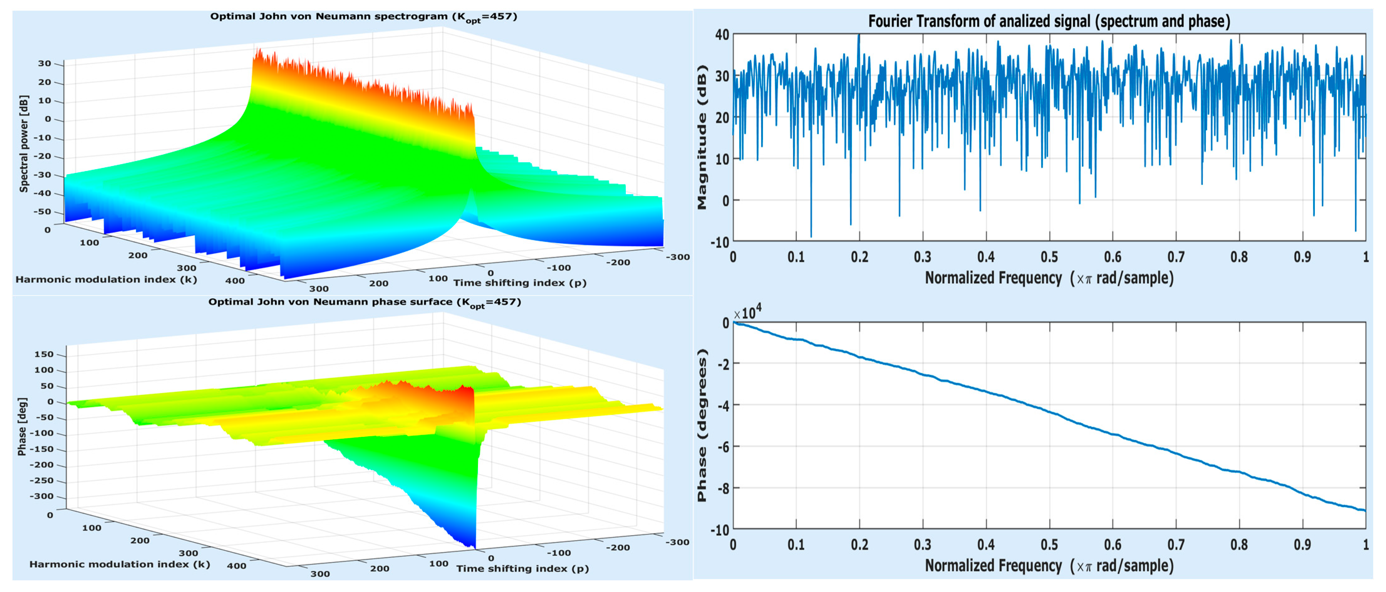
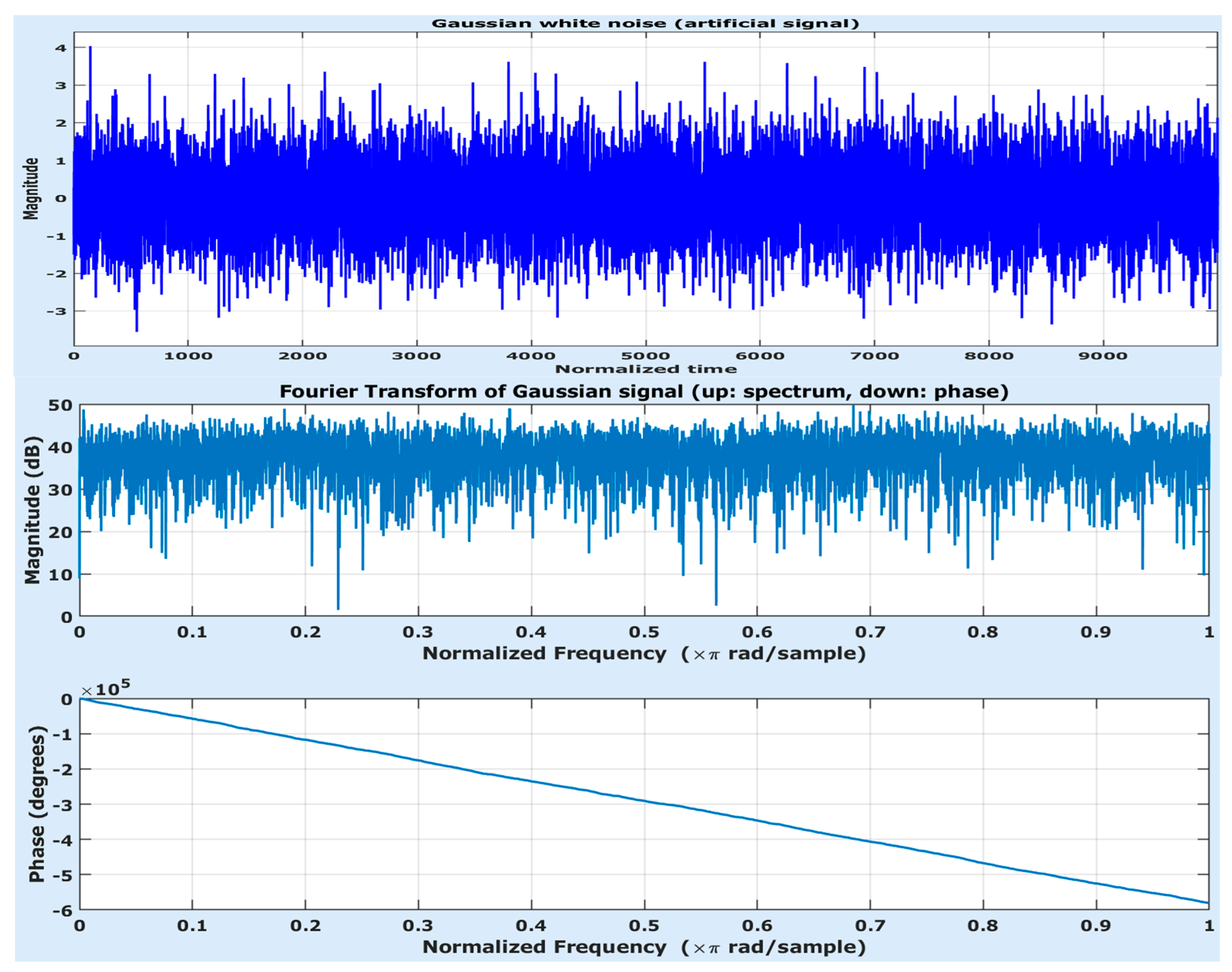
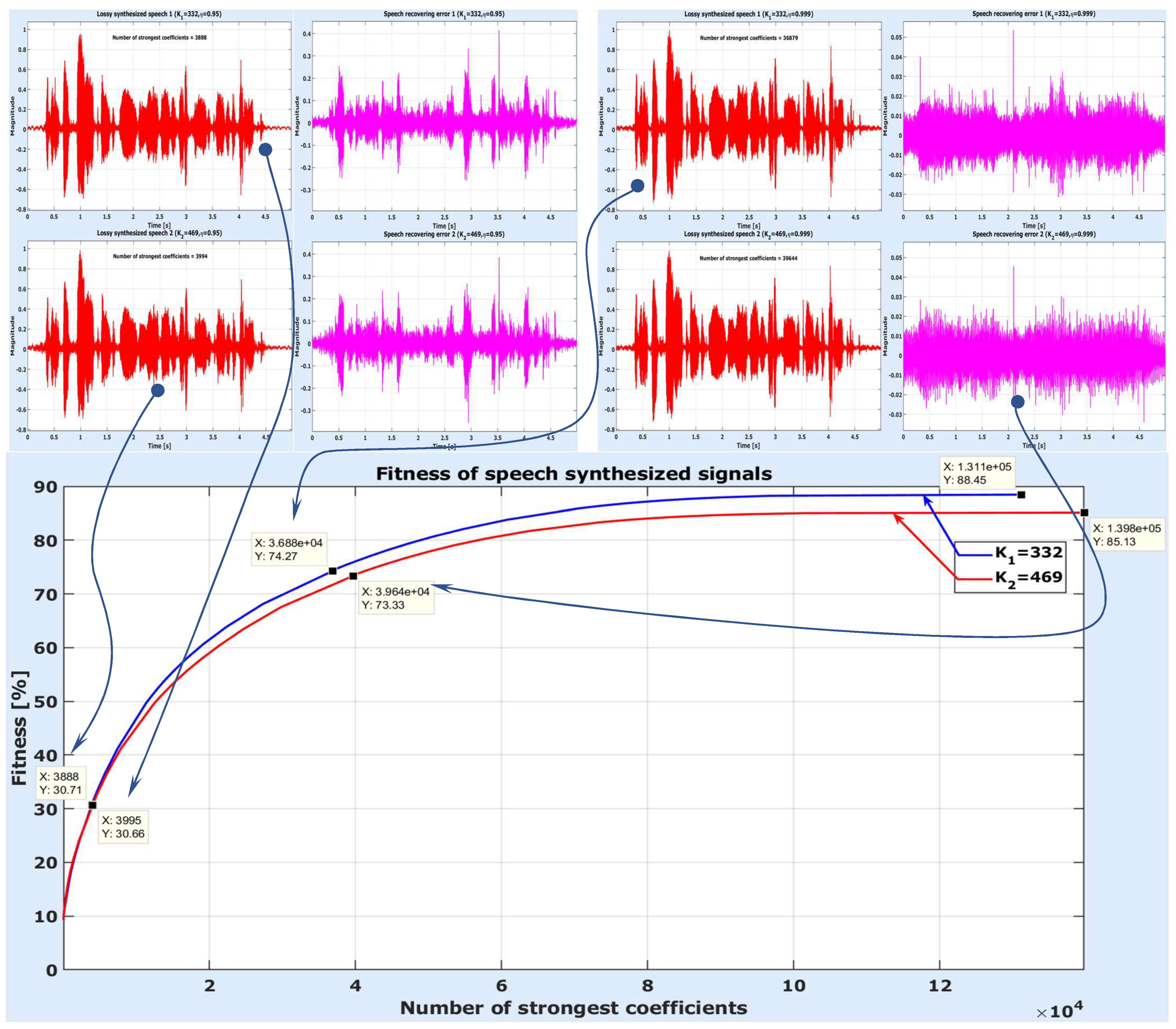
Table 1.
Performance parameters of JvNTs in the case of a Gaussian pseudo-random signal.
| Signal Length | Sampling Rate | Relative std of Error [%] | Accuracy [%] | Analysis Runtime [s] | Synthesis Runtime [s] |
|---|---|---|---|---|---|
| 1000 | 100 | 1.37 | 87.96 | 3.93 | 0.61 |
| 141 | 1.83 | 84.55 | 4.32 | 0.62 |
Table 2.
Relative energy versus JvN coefficients number for a speech signal.
| 20 | 25 | 30 | 35 | 40 | 45 | 50 | 55 | 60 | 65 | 70 | 75 | 80 | 85 | 90 | 95 | Angle | ||
|---|---|---|---|---|---|---|---|---|---|---|---|---|---|---|---|---|---|---|
| 30 | 48 | 74 | 107 | 149 | 204 | 268 | 340 | 424 | 521 | 642 | 799 | 1028 | 1426 | 2169 | 3888 | 17.60° | ||
| 26 | 43 | 65 | 92 | 124 | 162 | 210 | 268 | 336 | 422 | 531 | 686 | 926 | 1339 | 2110 | 3994 | 20.37° |
Table 3.
Performance parameters of JvNTs in the case of a speech signal.
| Signal Length | Sampling Rate | Relative std of Error [%] | Accuracy [%] | Analysis Runtime [s] | Synthesis Runtime [s] |
|---|---|---|---|---|---|
| 110,033 | 332 | 1.31 | 88.45 | 342.68 | 56.27 |
| 469 | 1.75 | 85.13 | 370.27 | 57.24 |
Disclaimer/Publisher’s Note: The statements, opinions and data contained in all publications are solely those of the individual author(s) and contributor(s) and not of MDPI and/or the editor(s). MDPI and/or the editor(s) disclaim responsibility for any injury to people or property resulting from any ideas, methods, instructions or products referred to in the content. |
© 2023 by the authors. Licensee MDPI, Basel, Switzerland. This article is an open access article distributed under the terms and conditions of the Creative Commons Attribution (CC BY) license (https://creativecommons.org/licenses/by/4.0/).
Share and Cite
MDPI and ACS Style
Stefanoiu, D.; Culita, J. John von Neumann’s Time-Frequency Orthogonal Transforms. Mathematics 2023, 11, 2607. https://doi.org/10.3390/math11122607
AMA Style
Stefanoiu D, Culita J. John von Neumann’s Time-Frequency Orthogonal Transforms. Mathematics. 2023; 11(12):2607. https://doi.org/10.3390/math11122607
Chicago/Turabian StyleStefanoiu, Dan, and Janetta Culita. 2023. "John von Neumann’s Time-Frequency Orthogonal Transforms" Mathematics 11, no. 12: 2607. https://doi.org/10.3390/math11122607
Note that from the first issue of 2016, this journal uses article numbers instead of page numbers. See further details here.