The Analysis of Risk Measurement and Association in China’s Financial Sector Using the Tail Risk Spillover Network

Abstract

This study focused on analyzing the complexities and risk spillovers that arise among financial institutions due to the development of financial markets. The research employed the conditional value at risk (CoVaR) methodology to quantify the extent of tail risk spillover and constructed a risk spillover network encompassing Chinese financial institutions. The study further investigated the characteristics, transmission paths, and dynamic evolution of this network under different risk conditions. The empirical findings of this research highlighted several important insights. First, financial institutions play distinct roles in the risk spillover process, with the securities and banking sectors as risk exporters and the insurance and diversified financial sectors as risk takers. The closest risk spillover relationships were observed between banking and insurance and between securities and diversified financial sectors. Second, in high-risk scenarios, there is significant intrasectoral risk transmission between banks and the diversified financial sector, as well as dual-sectoral risk contagion between banks and securities, with the most-common transmission occurring between diversified financial and securities sectors. Finally, the securities sector acts as the pivotal node for risk spillovers, being the main transmitter of intersectoral risks. The formation and evolution of risk spillover networks are influenced by endogenous mechanisms, in particular the convergence effect.

1. Introduction

Financial institutions play a crucial role in the functioning of the financial system. The advancement of financial innovation and liberalization has brought about close network relations among financial institutions, creating interdependence and interconnectedness. While this has led to increased efficiency in financial allocation, it has also increased the risk of instability in the financial system. Financial markets are inherently unstable due to fluctuations in asset prices and the transmission of volatility. This instability can quickly spread from one institution to another through interconnected channels, exacerbating systemic risks and potentially leading to a partial crisis that can spiral into a full-blown systemic crisis. The consequences of such a crisis can be devastating for the market as a whole, potentially causing significant harm to the economy and the public at large.

China’s financial system is undergoing a period of rapid growth characterized by increasing levels of mixed operations in the financial industry. The growing interconnectedness of the various financial sectors, including the banking, securities, insurance, and diversified finance sectors, is increasing the possibility for risk contagion. However, the current regulatory framework of China is not equipped to handle systemic risks effectively. The framework places a greater emphasis on the financial risks of individual institutions than on the overall risk flow pattern, making it difficult to prevent risk from spreading across the financial sector [1]. This is why studying the cross-sectoral risk spillover effects of Chinese financial institutions and understanding the nature of the networks formed among them is of significant academic value and importance in the context of ensuring a stable financial system. Thus, the findings of this research can contribute to improvements in regulatory policies and the development of more effective risk management strategies.

Contagion and risk spillover effects are two important characteristics of systemic risk. Traditional measures of systemic risk focus on changes in economic characteristics around the time that a risk arises and are used to construct a system of early warning indicators. The disadvantage of this approach is that it isolates the risks faced by individual financial institutions, but ignores the spillover effects of risk on other institutions, preventing the specific risks of an institution from being correctly assessed [2,3]. As research in this area continues to grow, new risk measurement techniques are being proposed (primarily indicators, including CoVaR, MES, and SRISK) and have become a topic of great interest in the field of financial risk measurement. The CoVaR and $\Delta$CoVaR measure the value at risk of a single financial institution to the system when financial markets are in crisis [4,5]. Jin [6] examined the risk contagion effect of China on the stock markets of Asian countries based on the CoVaR method with Copula functions and found that the trade links and investment flows between China and Asian economies exhibit a consistent trend in risk spillovers. Jian et al. [7] constructed a semiparametric CoVaR model that captured the two-way lag tail risk effect and found a significant two-way downside spillover effect between the Chinese stock and futures markets. Employing the CoVaR methodology, Bellavite Pellegrini et al. [8] used data from 476 financial institutions in Europe to analyze the correlation among the size, leverage ratio, and Beta values regarding their degree of contribution to systemic risk. Acharya et al. [9] proposed the MES, which represented the expected return of a single financial institution following losses from a financial crisis and the marginal contribution of a single institution to systemic risk. Brownlees and Engle [10] extended the MES to the systemic risk index (SRISK) to quantify the impact of systemic risk on capital shortfalls in financial institutions and found similarities in the results of the three indicators.

Bellavite Pellegrini et al. [11] employed the CoVaR, MES, and SRISK as measures of systemic risk for financial institutions to assess the impact of fundamental information on financial institutions on the level of systemic risk. The above risk measures focused on the interactions between financial institutions and the financial system; however, from a network perspective, they ignored the complex relationships among financial institutions, leading to a failure to capture the multisubject to multisubject risk spillover relationships from multiple entities to multiple entities in financial networks [3,12]. In the real financial system, such complex relationships are common, especially in the context of the Chinese stock market crash of 2015, when the prices of thousands of A-shares produced strong resonance phenomena. Therefore, we need to consider the risk spillover relationships among multiple agents [13].

The complex relationships among financial institutions become a vehicle for systemic risk, with the direction and intensity of risk spillovers being determined by associated patterns and structures [14]. As a result, the analysis of risk spillovers from the perspective of complex networks has become a new research tool in the field of financial risk. The focus of research has shifted to how to build a network of financial institutions that is similar to the real market. Financial institutions may be linked by multiple channels that encompass different forms of relationships, such as business partnerships (investments, loans, derivatives, futures contracts) and equity relationships (ownership, coinvestments, joint ventures, cross-shareholdings), which allows for overly redundant information about the construction of networks among financial institutions.

Some research work has focused on the construction of networks with asset–liability relationships [15,16]. The lack of transparency in the overall asset–liability relationships among financial institutions, the infrequency of updates, and the limitation to a specific form of association of assets and liabilities among financial institutions make such networks relatively unreliable. Financial market data and their fluctuations are the most-direct market performance indicators of financial institutions, with characteristics such as high frequency, a forward-looking orientation, and multichannel coverage; this means that the use of a network built on financial market data has a relatively high degree of credibility [17]. Most of the relevant studies have been based on market data with correlation coefficients and traditional measures used to construct networks of financial institutions.

Wang et al. [18] used the Pearson coefficients of market trading data as the main indicator of firm relevance, while product similarity was used as supplementary information for the construction of a network of firms based on a threshold selection approach to analyze structural differences in listed firms. In some literature, mutual information has been used to measure the correlation dependence among stock returns; for example, Yang et al. [19] used the mutual information of stock return series as a measure of dependence to extract a maximum spanning tree from the mutual information matrix, observing that the topology of the maximum spanning tree changed from star-like to chain-like after the crisis. Barbi and Prataviera [20] found that mutual information minimum spanning trees exhibit greater robustness and power-law tail properties in the degree distribution after a comparison with minimum spanning trees composed of mutual information and linear correlations, suggesting that they are relatively effective for measuring nonlinearities in financial markets. Gong et al. [14] proposed the use of principal component analysis and Granger causality networks to quantify interdependencies in the financial system, capturing the connectivity of the four sectors of finance and finding that the banking and insurance sectors play an important role in the formation and aggregation of systemic risk. Diebold and Yılmaz [21] constructed a high-dimensional network based on the VAR variance decomposition method and proposed net and gross volatility spillover indexes that not only portray the risk spillover relationship of financial institutions in the financial market, but also measure the overall risk level of the financial system. Using the volatility spillover analysis framework, Lundgren et al. [22] explored the source relationships of uncertainty among five different types of assets: energy, stocks, currencies, government bonds, and oil. Zeng et al. [23] and Ji et al. [24] studied the influencing factors of the volatility spillovers of virtual currencies and found that market size is not significantly correlated with volatility.

However, the above studies applied correlation and information spillovers to the field of risk spillovers. The tail-risk-driven network was proposed by Härdle et al. [25]. Networks constructed based on tail risk spillover effects can directly reflect changes in tail risk spillover, thus better capturing the path of risk contagion. Liu et al. [26] used the LASSO-CoVaR method to construct a tail risk network to assess the risk spillover effects of oil markets on the global financial system. There are few papers on the construction of tail risk networks to explore risk spillovers from financial institutions, and the literature on risk spillovers has focused too much on risk spillover relationships and contagion in the banking sector, ignoring other financial institutions. Against the backdrop of significantly increased risk spillovers across sectors, this approach undoubtedly underestimates the real impact that financial institutions bring to the table.

The structure of financial networks shows the distribution of individual financial institutions in the network, which can be used as an indicator to measure systemic risk [27] and to discuss the stability of the system and the efficiency of risk transmission [28,29]. In most related literature, the analysis of financial institution risk has relied on the topological indicators of the constructed networks, and comparisons of indicators reflect the characteristics of risk spillover relationships among financial institutions. The out-degree can reveal the extent of the impact of risk spillovers from a single institution [12,14,25]. The clustering coefficient reflects whether the risk spillover relationships among institutions are associative, making risk contagion deeper and more efficient [30]. Other metrics, such as centrality [31] and PageRank value [32], have also been used in these studies. Moreover, some scholars have explored the relevance of network topology indicators to financial market risk. Chen et al. [27] used a dynamic topology indicator to measure systemic risk. Li et al. [33] numerically simulated bank networks with different risk scenarios and found that as network connectivity increases, risks are effectively diversified, resulting in a downward trend in systemic risk.

Although a substantial amount of research has been conducted on topological indicators in the network of financial institutions, these studies are limited in their scope and reflect only single characteristics of the network. They tend to focus too much on individual financial institutions or provide only a relatively broad view of the network while failing to delve deeper into the finer details of association structures within financial institutions. The use of higher-order topological indicators and the identification of motifs is still relatively uncommon, leading to a lack of understanding of the relatively complex relationships within the network. This results in a gap in our understanding of the formation and evolution mechanism of the network. Thus, further research is needed to fully comprehend the intricacies of the association structure and how it changes over time.

Our work makes significant contributions to the field of financial risk analysis. First, we utilized the time-varying SJC-Copula-CoVaR method to effectively measure the tail risk of Chinese financial institutions and analyze the tail correlation and risk spillover characteristics among different sectors. Doing so provides valuable insights into the tail risk of financial institutions and their interconnections. Second, we constructed a tail risk spillover network for Chinese financial institutions, providing a comprehensive view of the risk transmission pathways among sectors. We identified the triad and four sectoral base motifs of the risk spillover network, explored the transmission paths of risks among sectors, and identified the sectors that play leading roles in the risk spillover process. This enables a deeper understanding of the relationships among financial institutions and the risks these relationships pose to the overall financial system. Finally, we innovatively used TERGM to explore the generation and evolutionary mechanisms of the networks of financial institutions. We examined the impact of the network topology on network evolution and investigated the coevolutionary properties of networks with different degrees of risk spillover. This provides important insights into the formation and evolution of the financial institution network and helps identify key factors that drive change over time.

Our work aimed to contribute valuable insights to risk management in financial institutions and the overall financial system. It provides a deeper understanding of tail risk, risk spillover, network formation, and evolution, facilitating informed decision-making and enhancing the stability and resilience of the financial system.

This paper consists of the following sections. In Section 2, we describe the selection and characteristics of the data. The main models and methods used are outlined in Section 3. Section 4 presents the empirical analysis, and Section 5 concludes the paper.

2. Data Description

Sectoral cluster effects are common in financial networks. To study changes in intersectoral financial risk spillover relationships, we refer to the results of other works [34,35] and the actual situation in China’s financial market and divided financial institutions into four categories: banking, securities, insurance, and diversified institutions. The former three are the major traditional components of the overall financial sector, and the latter refers to all other financial sectors, including trusts, Internet finance, and consumer finance.

To fully reflect the basic characteristics, actual situation, and market state of each financial sector and to ensure the reliability and integrity of the data, 63 listed financial institutions in China were selected as the research object; the total market value and trading volume of these institutions account for more than 80% of the financial sector, and such coverage is typically considered representative and able to reflect the overall characteristics of the risk spillover of financial institutions.

To measure the risk spillover relationships among financial sectors, we selected a sample interval including a total of 2155 observation samples from 11 January 2011 to 31 December 2020, at a daily frequency, and the forward compounded closing price was used for the stock prices of the financial institutions (the data source was the Wind database). The selected time period from 11 January 2011 to 31 December 2020 was chosen for several reasons. Firstly, it provides a sufficient length of approximately ten years, allowing for a substantial sample size for analysis. This extended duration enabled us to observe and analyze long-term trends, cyclicality, and potential structural changes in the financial markets. Additionally, by incorporating data up to 31 December 2020, we ensured that our analysis included recent market developments, accounting for any potential shifts or events that may have occurred in the financial system. This helped to capture the most up-to-date information available and enhance the relevance of our findings. Furthermore, the selected time period aligns with previous studies and research conducted in the field, ensuring comparability and facilitating building upon prior findings. Overall, these considerations support the robustness and validity of our analysis within the chosen time frame.

The yield series is calculated according to the following formula:

$$R_{it}=ln(P_{it}/P_{it-1})$$

where $P_{it}$ represents the closing price of financial institution i at time t.

We counted the basic characteristics of the financial sector yield series. As shown in

Table 1. Descriptive statistics for the financial sector yield series.

	Mean	Standard Deviation	Maximum	Minimum	Skewness	Kurtosis	Jarque–Bera	Ljung–Box
Banking	$0.049$	$1.342$	$7.573$	$-9.116$	$0.227$	$10.460$	$4988.93$ ***	$76.41$ ***
Securities	$0.078$	$2.041$	$8.757$	$-8.882$	$0.088$	$6.538$	$1119.70$ ***	$46.10$ ***
Insurance	$0.071$	$1.888$	$9.818$	$-9.407$	$0.216$	$6.023$	$831.81$ ***	$61.67$ ***
Diversified	$0.059$	$1.702$	$8.219$	$-8.582$	$-0.538$	$6.077$	$948.73$ ***	$51.20$ ***

*** represents the significance of the Jarque–Bera and Ljung–Box values at the 1% levels.

, the average returns of each financial sector are positive during the sample period; the return rate of the banking sector fluctuates the least, and the return rate of the securities sector fluctuates the most. As seen from the skewness and kurtosis, the returns of diversified financial institutions showed a left-skewed profile, and the remaining financial sectors showed a right-skewed profile.

Skewness refers to the asymmetry of a distribution. A positive skewness indicates a longer tail on the right side, while a negative skewness indicates a longer tail on the left side. In this case, it was found that the returns of diversified financial institutions exhibited a left-skewed profile. This means that the distribution of returns for these institutions had a longer left tail and was skewed towards the negative side. This suggested that there may be more occurrences of lower or negative returns for diversified financial institutions. On the other hand, the remaining financial sectors showed a right-skewed profile. This indicated that their returns had a longer right tail and were skewed towards the positive side. This suggested that these sectors may experience more instances of higher or positive returns. Kurtosis, on the other hand, measures the thickness of the tails of a distribution. Higher kurtosis implies fatter tails, indicating a higher probability of extreme events or outliers compared to a normal distribution. The returns across all financial sectors exhibited pronounced peaks and fat tails, indicating inefficiency in return volatility within this financial market. In other words, there was a higher likelihood of extreme events or outliers occurring in the returns compared to what would be expected under a normal distribution. The presence of fat tails suggested that there may be more instances of large gains or losses in the financial market, indicating a higher level of risk and potentially nonlinear relationships between different variables affecting returns.

The Jarque–Bera statistic was used to test the assumption that the returns of the financial sectors follow a normal distribution. The rejection of the original hypothesis of normality for all sectors implied that the returns do not conform to a traditional bell-shaped curve. This suggested that the returns exhibited significant deviations from a normal distribution and may display more extreme or non-standard patterns. The Ljung–Box statistic was employed to assess the presence of autocorrelation or serial dependence in the series of returns. The finding that all series exhibited fluctuating aggregation indicated that there was the presence of temporal dependence or autocorrelation in the returns of all sectors. This suggests that the past values of returns had a significant influence on future returns, indicating patterns of persistence or clustering in the data.

The non-normality of the returns highlighted the need for caution when using traditional statistical methods that assume normality in the financial sector. This suggested that alternative models may be required to capture the unique characteristics and patterns present in the returns. The presence of fluctuating aggregation indicated that there were persistent patterns in the returns, which can have implications for risk management and forecasting. Understanding and modeling the autocorrelation in the returns becomes crucial for accurately estimating risks and predicting future movements in the financial market.

3. Research Methods

3.1. Risk Spillover Measure

The CoVaR method, which was proposed by Tobias and Brunnermeier [4] and draws on the core ideas of the VaR method to measure the extent to which institutions and industries contribute to systemic risk [5] and to examine risk transmission and spillovers among multiple financial institutions [36], was used as a theoretical framework for risk contagion analysis in this paper.

There are currently three main types of representative approaches to CoVaR estimation: the quantile regression method [4,37,38], the DDC-GARCH model [39,40], and the Copula model [41]. The CoVaR method based on the Copula model is increasingly being used to measure systemic risk in financial institutions due to its ability to measure asymmetric risk characteristics and examine the tail dependence structure of variables; moreover, the Copula method further extends static framework analysis to dynamic framework analysis to enable better examinations of the time-varying nature of systemic risk spillover effects in financial institutions [42]. Therefore, this paper integrated the GJR-GARCH and SJC-Copula models into the CoVaR framework. As the GARCH model captures the typical characteristics of the volatility of financial institutions and the Copula function can characterize the dependency structure among financial institutions, a combination of the two can effectively measure the time-varying risk spillover relationships among financial institutions.

3.1.1. Marginal Distribution Fitting: The GARCH Model

To enhance the accuracy of our analysis, we adopted the AR(1)-GJR-Skew(t) model to estimate the edge distribution of each financial institution’s return series, which is a crucial step in using the Copula function to identify the tail dependence structure among financial institutions. The use of traditional GARCH models is limited in this context, as such models are equipped to handle only normally distributed financial return series, while the actual return series of financial assets exhibited more complex characteristics, such as spikes, biases, heteroskedasticity, and leverage effects. On the other hand, the AR(1)-GJR-Skew(t) model considers these characteristics and provides a relatively comprehensive characterization of the volatility of each financial institution, thereby ensuring the validity of our analysis and the robustness of our results. The mean equation, variance equation, and residual distribution of the AR(1)-GJR-Skew(t) model are

$$\begin{array}{c}\hfill \begin{array}{cc}\hfill r_{i,t}& =c_0+c_1{R}_{i,t-1}+e_{i,t}\hfill \\ \\ \hfill e_{i,t}& =h_{i,t}{\epsilon }_{i,t},{\epsilon }_{i,t}\sim SKT(v,\lambda )\hfill \\ \\ \hfill h_{i,t}& ={\omega }_{i,t}+\alpha e_{i,t-1}^2+\beta h_{i,t-1}+\gamma e_{i,t-1}^{2}I\left(e_{i,t-1}<0\right)\hfill \end{array}\end{array}$$

(1)

where $r_{it}$ denotes the return series of financial institution i, $e_{i,t}$ is a random disturbance term that obeys the skewed t-distribution of the independent identical distribution, $h_{i,t}^2$ is the conditional variance, v is the kurtosis parameter, and $\lambda$ is the asymmetry parameter. $I\left(e_{i,t-1}<0\right)$ is an indicative indicator. When $e_{i,t-1}<0$, I equals 1; otherwise, I equals 0, indicating that the volatility of the return series in the face of a negative shock is greater than that in the face of a positive shock.

3.1.2. Tail Dependence Measure: SJR-Copula Model

The use of the Copula function is widely accepted in financial risk measurement to characterize the joint distribution of variables. Sklar’s description of the Copula link function explains how it connects the joint distribution of random variables to the marginal distribution, enabling the creation of any two-dimensional joint distribution function by linking it to the corresponding marginal distribution.

$$F(x,y)=C\left(F\right(x),G(y\left)\right)$$

(2)

where $C(·,·)$ is the Copula-dependent structure.

The time-varying SJC-Copula model is a good choice for describing the risk dependence structure among financial institutions due to its several benefits. First, the model is relatively nonrestrictive and does not require that the joint distribution form be specified, making it easier to determine the marginal distribution and choose the appropriate Copula model. Second, the model is capable of capturing more accurately the nonlinear and heavy-tailed risk dependence characteristics among financial institutions’ return series than are other methods, such as Pearson correlation coefficients or Granger causality tests. Third, the model is designed to account for the time-varying nature of financial market dependencies and can accurately reflect tail dependencies in various market scenarios, including positive and negative events [43,44], by providing a comprehensive analysis of the dynamic upper- and lower-tail dependency coefficients among financial institutions.

The distribution function of the SJC-Copula function is:

$$\begin{array}{cc}\hfill C_{SJC}(u,v)=& \frac{1}{2}\left\{1-{\left\{1-{\left\{{\left[1-{(1-u)}^{\kappa }\right]}^{-\gamma }+{\left[1-{(1-v)}^{\kappa }\right]}^{-\gamma }-1\right\}}^{-\frac{1}{\gamma }}\right\}}^{-\frac{1}{\kappa }}+\right.\hfill \\ \hfill & \left.{\left\{1-{\left[{\left(1-u^{\kappa }\right)}^{-\gamma }+{\left(1-v^{\kappa }\right)}^{-\gamma }-1\right]}^{-\frac{1}{\gamma }}\right\}}^{-\frac{1}{\kappa }}+u+v\right\}\hfill \end{array}$$

(3)

The time-varying SJC-Copula function is a dynamic evolution process of its relational parameters based on the SJC-Copula function. Patton [45] suggested that current correlations can be explained by the historical correlations and historical averages of the cumulative probabilities of the focal variables, namely by using a process similar to ARMA(1,10) to describe the dynamic tail dependence coefficients. Considering that the time-varying SJC-Copula function proposed by Patton may be biased in describing the cotrend between two random sequences, Chen et al. [46] improved the dynamic evolution relation of the tail dependence coefficient $\tau$ proposed by Patton and then obtained the improved dynamic evolution equation of the tail dependence coefficient $\tau$ as follows:

$$\begin{array}{cc}\hfill {\tau }_t^U& =\Lambda \left({\omega }_U+{\beta }_U{\tau }_{t-1}^U+{\alpha }_U\times \frac{1}{q}\sum _{i=1}^q\left|u_{1t-i}-u_{2t-i}\right|\right)\hfill \\ \hfill {\tau }_t^L& =\Lambda \left({\omega }_L+{\beta }_L{\tau }_{t-1}^L+{\alpha }_L\times \frac{1}{q}\sum _{i=1}^q\left|u_{1t-i}-u_{2t-i}\right|\right)\hfill \end{array}$$

(4)

where $\Lambda (·)$ is a $logistic$ transformation function that ensures that the tail-dependent parameters lie within the interval $(0,1)$ and is defined as $\Lambda \left(x\right)=\frac{1}{1+e^{-x}}$.

3.1.3. Risk Spillover Measure: CoVaR Model

The CoVaR method indicates that, at a certain probability level, when the loss of an institution at a specific time in the future equals the VaR, the maximum loss of other institutions is:

$$Pr\left(X^j\le CoVa{R}_q^{j|i}\mid X^i=Va{R}_q^i\right)=q$$

(5)

$CoVa{R}_q^{j|i}$ reflects the total value at risk of institution j, comprising the unconditional value at risk and the value of the risk that spills over to it from institution i. To measure the absolute value of the risk spillover contribution of institution i to institution j, the value of the spillover risk is defined as

$$\Delta CoVa{R}_q^{j|i}=CoVa{R}_q^{j|i}-CoVa{R}_q^{j|i=Median}$$

(6)

To remove the influence of the dimension and, thus, facilitate comparisons among different financial institutions to fully reflect the intensity of the risk spillover effect, we can standardize the value at risk of spillovers. This value represents the intensity of risk spillover, which reflects the relative ratio of the incremental risk faced by financial institution j that is induced by financial institution i on the risk of financial institution j. The %CoVaR contains more information and is more informative than the $\Delta$CoVaR.

$$\%CoVa{R}_q^{j|i}=\frac{\Delta CoVa{R}_q^{j|i}}{CoVa{R}_q^{j|i=Median}}$$

(7)

3.2. Risk Spillover Networks

The increasing interconnectedness of financial institutions in China due to financial relationships has led to the formation of complex financial networks, through which risks can be transmitted through spillovers from one institution to another. The study of spillover networks offers a comprehensive understanding of the flow and extent of risk contagion in the financial industry. By utilizing the complex network framework, the relationships and dependencies among financial institutions can be relatively accurately represented, providing valuable insights into the transmission of risks and their impact on the overall stability of the financial system. The analysis of spillover networks serves as an essential tool for monitoring and managing systemic risks in the financial sector, helping to mitigate the potential for negative outcomes and promote stability in the financial industry. We refer to the research ideas of Hautsch et al. [3], Martinez-Jaramillo et al. [47], Huang et al. [48] and provide the risk spillover matrix among financial institutions at time t in

Table 2. The risk spillover matrix.

	$r_1$	$r_2$		$r_n$	To
$r_1$	0	$d_{12}$	⋯	$d_{1n}$	${\sum }_{j=1}^n{d}_{1j}$
$r_2$	$d_{21}$	0	⋯	$d_{2n}$	${\sum }_{j=1}^n{d}_{2j}$
⋯	⋯	⋯	⋯	⋯	⋯
$r_n$	$d_{n1}$	$d_{n2}$	⋯	0	${\sum }_{j=1}^n{d}_{nj}$
From	${\sum }_{i=1}^n{d}_{i1}$	${\sum }_{i=1}^n{d}_{i2}$	⋯	${\sum }_{i=1}^n{d}_{in}$	TC

in conjunction with the risk spillover effect %CoVaR measured above.

$d_{ij}=\%CoVa{R}_q^{j|i}$ represents the standardized marginal risk spillover effect of financial institution i on financial institution j at time t. By summing the jth column of the adjacency matrix of the risk contagion network, we can obtain the total systemic financial risk overflow level $TI{C}^{\mathrm{From}}$ of financial institution j. Moreover, the total spillover level $TI{C}^{\mathrm{To}}$ of systemic financial risk from financial institution i to all other institutions can be obtained by adding the ith row of the adjacency matrix of the risk contagion network. Furthermore, all elements of the risk spillover matrix are normalized and summed to obtain the total level TC of systemic financial risk, i.e.,

$$\begin{array}{c}{\mathrm{TIC}}^{\mathrm{To}}=\sum _{\mathrm{i}=1}^{\mathrm{n}}{\mathrm{d}}_{\mathrm{ij}}\hfill \\ \\ {\mathrm{TIC}}^{\mathrm{From}}=\sum _{\mathrm{j}=1}^{\mathrm{n}}{\mathrm{d}}_{\mathrm{ij}}\hfill \\ \\ \mathrm{TC}=\frac{{\sum }_{\mathrm{i},\mathrm{j}=1}^{\mathrm{n}}{\mathrm{d}}_{\mathrm{ij}}}{\mathrm{n}}=\frac{{\sum }_{\mathrm{i}=1}^{\mathrm{n}}{\mathrm{TIC}}^{\mathrm{To}}}{\mathrm{n}}=\frac{{\sum }_{\mathrm{j}=1}^{\mathrm{n}}{\mathrm{TIC}}^{\mathrm{From}}·}{\mathrm{n}}\hfill \end{array}$$

(8)

However, while the risk spillover matrix provides a comprehensive view of the interconnections within the financial industry, it can be difficult to interpret and analyze. The level of risk spillover is a crucial factor in determining the level of risk correlation and potential impact among financial institutions. To address this issue, this paper used a percentile-based approach to categorize the risk spillover matrix into three levels: high-, moderate-, and low-risk spillover networks. This categorization process allows for a more intuitive understanding of risk spillover relationships and provides a framework for multilevel analysis of the spillover network. The results of this categorization are presented in

Table 3. The setting of risk spillover.

The Degree of Risk Spillover	Percentile	The Network Relation ($\mathit{i}\to \mathit{j}$)
High	Top 30%	The value is 1; otherwise, it is 0
Moderate	30–60%	The value is 1; otherwise, it is 0
Low	60–100%	The value is 1; otherwise, it is 0

and reveal a clear division among the various levels of risk spillover.

In this paper, three types of risk spillover networks—high, moderate, and low—were constructed through threshold filtering, and the topological characteristics of each network were further analyzed (see

Table 4. Topology properties of the network.

Index	Function	Diagram
Density	The ratio of extant edges to potential edges
Reciprocity	The ratio of bidirectional edges to all edges
Cluster coefficient	The degree to which nodes tend to cluster together
Betweenness centrality	The proportion of nodes that are intermediaries

).

3.3. Research on Network Generation and Evolutionary Mechanisms

In general, the generation and evolution of networks are influenced by a variety of social processes, including both exogenous and endogenous mechanisms, which influence the formation of networks with a particular structure [49]. The social process of network self-organization can be understood as follows: network relationships can form certain network patterns through the self-organization process, thus promoting the formation of other network relationships. These local network patterns are called network structures and are endogenous effects. The exogenous mechanism includes the actor attributes of network nodes and exogenous scenarios. Actor attributes are divided into sender effects, receiver effects, and convergence or divergence between senders and receivers; moreover, exogenous situational factors include the entrainment effects of other networks [49]. In relation to a financial institution’s risk spillover network, an exogenous mechanism refers to the financial institution’s ability to affect the individual information generated by the network, and an endogenous mechanism refers to the law of network self-evolution in the risk spillover network. Traditional logistic models ignore the influence of the network structure on the formation of network relationships. The time-exponential random graph model (TERGM) is an econometric model of relationship data in complex networks that can be used to investigate the influence of exogenous and endogenous mechanisms on network connectivity to test whether an observed network structure is consistent with hypothesized trends [50,51,52]. Therefore, based on the risk spillover network constructed by the SJC-Copula-CoVaR, a TERGM was used to empirically analyze the evolutionary dynamics and influence mechanisms of the risk spillover network in terms of exogenous and endogenous mechanisms.

The general form of the TERGM is:

$$P(Y=y|\theta )=(1/k)exp\left\{{\theta }^{T}Z\left(y\right)+{\theta }_A^T{z}_a(y,x)\right\}$$

(9)

The normalized parameter k ensures that the network structure probability y falls between 0 and 1. $\theta$ represents the coefficient of the internal network structure statistic $z\left(x\right)$, and ${\theta }_A$ refers to the attribute statistic $z_a(y,x)$ of the network node. The magnitude and direction of the estimated parameters indicate the level and trend of the corresponding statistic’s influence on the generation and evolution of the network.

In this research, the focus was on the endogenous mechanism of the risk spillover network of the financial industry as explained through the lens of complex network theory. This theory highlights the importance of both structure-dependent effects (such as reciprocity, convergence, transmission, and connectivity) and time-dependent effects (such as stability and variability) in shaping the risk spillover network.

To understand the impact of these factors on the network, the authors of this paper drew from existing network generation and evolution theories and proposed six hypotheses. These hypotheses were based on the results of a network topology analysis that suggested that the financial network has structural properties, such as reciprocity, convergence, transmission, and connectivity, and time-dependent properties, such as stability and variability. To test these hypotheses, the authors used a TERGM to perform empirical analyses, investigating the interplay between these structural and time-dependent properties and their impacts on the evolution of the risk spillover network.

3.3.1. Structure-Dependent Effects

Reciprocity is an important feature of directed networks that explains the relationships formed by nodes through feedback. Reciprocity is a measure of the simplest interaction processes occurring in the network and is widely used when modeling complex networks [53]. Garlaschelli and Loffredo [54] found that the detection of reciprocity helps reveal the formation mechanisms of the observed network topology and explain its organization principles. In a risk spillover network, one institution has a risk spillover effect on another institution, and the connection between the two institutions is closed and prone to synchronous resonance, making the risk spillover interaction two-way in nature [55]. Therefore, the following is proposed:

Hypothesis 1.

There is a reciprocal effect in the risk spillover network that is evidenced by the tendency for financial institution risk spillovers to form reciprocal relationships.

Convergence is a key endogenous mechanism driving the dynamic evolution of networks and was first proposed by Barabási and Albert [56]. Convergence was then gradually applied to the study of networks with the aim of constructing relational models to reveal the evolutionary characteristics of network structures. Convergence means that network nodes tend to connect with nodes that have more connections, thus contributing to the formation of a network. Due to factors such as business linkages, financial institutions can be divided into receivers and exporters in the risk communication process. When an institution is at the center of a network, it can have an impact on most of the remaining institutions, creating a convergence effect [57]. Therefore, we propose the following:

Hypothesis 2.

There is a convergence effect in the risk spillover network, i.e., the presence of subjects in the risk spillover network generates risk spillovers and overflows to a large number of the remaining institutions.

Transmissibility refers to the ease with which the network node connections form triadic transmission closures, allowing for the creation of tighter communities within the network. Empirical evidence suggests that triadic transfer closure is an important endogenous mechanism that influences relationship selection and drives network cluster formation [58]. In a risk spillover network, close cooperation or business similarities among financial institutions can lead to the creation of communities in which risk spillover relationships tend to be closed. On the other hand, listed companies may hold shares in each other for specific purposes, creating cross-shareholding relationships. Guo et al. [59] studied cross-shareholdings in listed companies and found that cross-shareholding behavior can feature embedded social network patterns that contribute to the formation of transmission effects. Therefore, we propose the following:

Hypothesis 3.

There is a transmission effect in the risk spillover network, i.e., there is a tendency for risk spillovers among financial institutions to form a triad of transmission closures.

Connectivity is one of the more specific network constructs in the network, meaning that relationships connect two nodes through one or more third-party nodes. In risk spillover networks, connectivity is reflected in the existence of multiple paths for the transmission of risk spillover to achieve the transmission of indirect spillover relationships, accelerating the risk spillover. Therefore, the following is proposed:

Hypothesis 4.

There is a contagion effect in the risk spillover network, i.e., risk spillovers tend to take multiple paths among financial institutions.

3.3.2. Time-Dependent Effects

A dynamic network relationship can continue to evolve over time. On the one hand, this relationship manifests in the emergence of new nodes and the death of nodes. On the other hand, this relationship manifests in the change in connections among nodes. Due to the limitations of our research model and data, this paper discusses only the latter. Lusher et al. [49] suggested that the passage of time tends to have two effects on the generation and evolution of network relationships: in one effect, the relationship from the previous stage remains in each new stage; in the other effect, a change in the relationship occurs with the arrival of each stage. In a risk spillover network, the formation and maintenance of financial institution relationships may incorporate both long-term factors together—the external relationships of financial institution entities—and short-term factors—changes in the market environment—both of which drive the dynamic evolution of the network. Therefore, we propose the following:

Hypothesis 5.

Risk spillover networks have stability, i.e., risk spillover network relationships have path-dependent characteristics.

Hypothesis 6.

Risk spillover networks have variability, i.e., risk spillover network relationships tend to change over time.

Consequently, in this paper, we considered the structure-dependent effects—reciprocity, dependence, transmission, and connectivity—and the time-dependent effects—stability and variability—which have strong explanatory power for the generation and evolution of risk spillover networks. We chose the seven network structures shown in

Table 5. Network high-order statistics.

	Index	Function	Diagram
	edges		Basic directed network relationship
	mutual		Network relationships have feedback
Structure- dependent effects	gwideg		Network nodes have convergence
	transity		Network forms triadic transmission closures
	gwdsp		Network has multipath nodes
Time- dependent effects	stability		Network has path dependency
	variability		Network is time-varying

for the network statistics.

3.3.3. Network Node Properties

In addition to the endogenous network structure variables described above, the TERGM model can incorporate node attributes and interaction terms into the analysis. Node attributes represent the individual characteristics of network nodes, which measure whether an institution with specific properties tends to accept/reject more risk spillover relationships than other institutions [60]. In this paper, important exogenous institutional influences were added to the model, including earnings per share (epsTTM), the debt-to-asset ratio (reliabilityToAsset), net profit growth (YOYNI), and net profit (npMargin). In contrast, interaction terms for node attributes are concerned with the interaction characteristics of two members of a binary group, the most-common interaction term being the homogeneity problem between the two members of the binary group. There are four types of financial institutions in this paper: banking, securities, insurance, and diversified financial. To test whether there is a stronger risk spillover effect among financial institutions in the same sector, a certain interaction term—homogeneity (industry)—was added to the model. In addition, different levels of risk spillover networks from the previous period were included in the model to measure the evolution of their relationships.

In summary, in this paper, the following model is constructed:

$$\begin{array}{cc}\hfill Pr\left(E_{ij}\right)=& \frac{1}{c}exp({\theta }_{0}edges+{\theta }_{1}mutual+{\theta }_{2}gwideg+{\theta }_{3}gwesp+{\theta }_{4}gwdsp+\hfill \\ \hfill & {\theta }_{5}stability+{\theta }_{6}variability+{\theta }_{7}industry+{\theta }_{8}epsTTM+\hfill \\ \hfill & {\theta }_{9}liabilityToAsset+{\theta }_{10}YOYNI+{\theta }_{11}npMargin+{\theta }_{12}covnet)\hfill \end{array}$$

(10)

4. Empirical Results

4.1. Measurements of Systemic Risk Spillover Effects from Financial Institutions

4.1.1. Marginal Distribution Model Fitting Results

We chose the GARCH(1,1) model for the following reasons: First, GARCH(1,1) models are relatively simple and computationally efficient compared to higher-order GARCH models. They have a smaller number of parameters to estimate, which is advantageous when dealing with limited data or limited computational resources. Furthermore, empirical studies have widely utilized GARCH(1,1) models and have demonstrated their effectiveness in capturing volatility patterns in various financial time series. They provide reasonably accurate and robust estimates of volatility in practical applications. Finally, GARCH(1,1) models strike a balance between capturing the persistence of volatility (ARCH effect) and the short-term volatility reaction (GARCH effect). Higher-order GARCH models with larger values of p and q tend to introduce unnecessary complexity without substantial improvements in forecasting performance.

To obtain the parameters of the ARMA (1,0)-GJR-GARCH (1,1) model, we employed a two-step approach. First, we estimated the parameters of the ARMA (1,0) model using the method of maximum likelihood estimation (MLE). This was performed by minimizing the negative log-likelihood function associated with the ARMA model. The resulting ARMA parameters were then used as inputs for the subsequent estimation of the GJR-GARCH (1,1) parameters. Second, we estimated the parameters of the GJR-GARCH (1,1) model using the conditional maximum likelihood estimation (cMLE) approach. This estimation method took into account the conditional heteroscedasticity and asymmetric effects in the data. The GJR-GARCH (1,1) model allows for time-varying volatility and captures the leverage effect often observed in financial time series data. We utilized the GARCH (1,1) specification to effectively model the volatility dynamics in our study.

When using numerical optimization algorithms to maximize the likelihood function and estimate the parameters of an ARMA(1,0)-GJR-GARCH(1,1) model, several techniques have been employed to enhance convergence: (a) optimization algorithm selection: the iterative Quasi-Newton algorithm, which is an extension of the Broyden–Fletcher–Goldfarb–Shannon (BFGS) method for nonlinear optimization, was used in GARCH model estimation; (b) constraints and bounds: setting appropriate constraints and bounds on the parameters; (c) convergence criteria: specify convergence criteria that determine when to stop the optimization process. The criteria are based on the maximum number of iterations.

The results of the parameter estimation in

Table 6. Parameter estimation results for ARMA (1,0)-GJR-GARCH (1,1).

	Banking	Securities	Insurance	Diversified
$c_0$	$0.0606$ ***	$0.0205$	$-0.0732$ **	0.0196
$c_1$	$-0.0199$	$-0.0231$ **	$-0.0156$	$0.0506$ **
$\omega$	$0.0303$ ***	$0.0393$ **	$0.0281$ *	$0.0300$ **
$\alpha$	$0.0593$ ***	$0.0572$ ***	$0.0596$ ***	$0.0688$ ***
$\beta$	$0.9078$ ***	$0.9373$ ***	$0.9352$ ***	$0.9186$ ***
$\gamma$	$-0.0225$ *	$-0.0112$ *	$0.0025$ *	$0.01043$ **
v	$3.3025$ ***	$3.4708$ ***	$4.7907$ ***	$5.4532$ ***
$\lambda$	$0.1437$ ***	$0.0348$	$0.1154$ ***	$-0.1334$ ***
$LL$	$-3140.982$	$-4233.006$	$-4153.916$	$-3870.935$
$AIC$	$6297.964$	$8482.013$	$8323.833$	$7757.869$
$BIC$	$6343.469$	$8527.418$	$8369.237$	$7803.274$

***, **, * represent the significance of t-statistics values at the $1\%$, $5\%$, $10\%$ levels, respectively.

show that the GARCH term parameter $\alpha +\beta$ was greater than 0.9, which indicated that financial market volatility was highly aggregated; that is, the characteristics of strong persistence and prolonged memory were present. The $\alpha$ coefficients for the securities and insurance sectors were slightly lower than those for the banking and diversified sectors, and the $\beta$ coefficients were slightly higher, indicating that the securities and insurance sectors were less information-sensitive and relied heavily on their memorability for market fluctuations. The parameter $\gamma$ of the asymmetric effect term clearly showed that all four financial sectors were characterized by asymmetric volatility in the face of external information shocks, with leverage effects. The insurance and diversified sectors were more exposed to negative news, while the banking and securities sectors were more vulnerable to positive news. In addition, the estimates of the skewness parameter v and the shape parameter $\lambda$ illustrated the significant asymmetry and thick tails of the distribution of the standard residual series of each financial sector.

The results of the parameter estimation in Table 6 revealed intriguing insights into the nature of volatility in financial markets. As the GARCH term parameter $\alpha +\beta$ was greater than 0.9, the financial market volatility was shown to be highly persistent and exhibited prolonged memory, meaning that past events had a lasting impact on the present. Furthermore, a comparison of the $\alpha$ coefficients between the securities and insurance sectors and the banking and diversified sectors revealed that the former was less information-sensitive and heavily relied on its memorability to adapt to market fluctuations. The presence of an asymmetric effect term, represented by the parameter $\gamma$, highlighted that all four financial sectors were characterized by asymmetric volatility in response to external information shocks, displaying leverage effects. The insurance and diversified sectors were more vulnerable to negative news, while the banking and securities sectors were more susceptible to positive news. Additionally, the estimates of the skewness v and shape $\lambda$ parameters further reinforced the notions of significant asymmetry and thick tails in the distribution of the standard residual series of each financial sector. These results provided a comprehensive and nuanced understanding of the financial market’s volatility dynamics, emphasizing the importance of considering both persistence and asymmetry in the contexts of risk management and decision-making.

4.1.2. Results of the Tail Dependence Measures

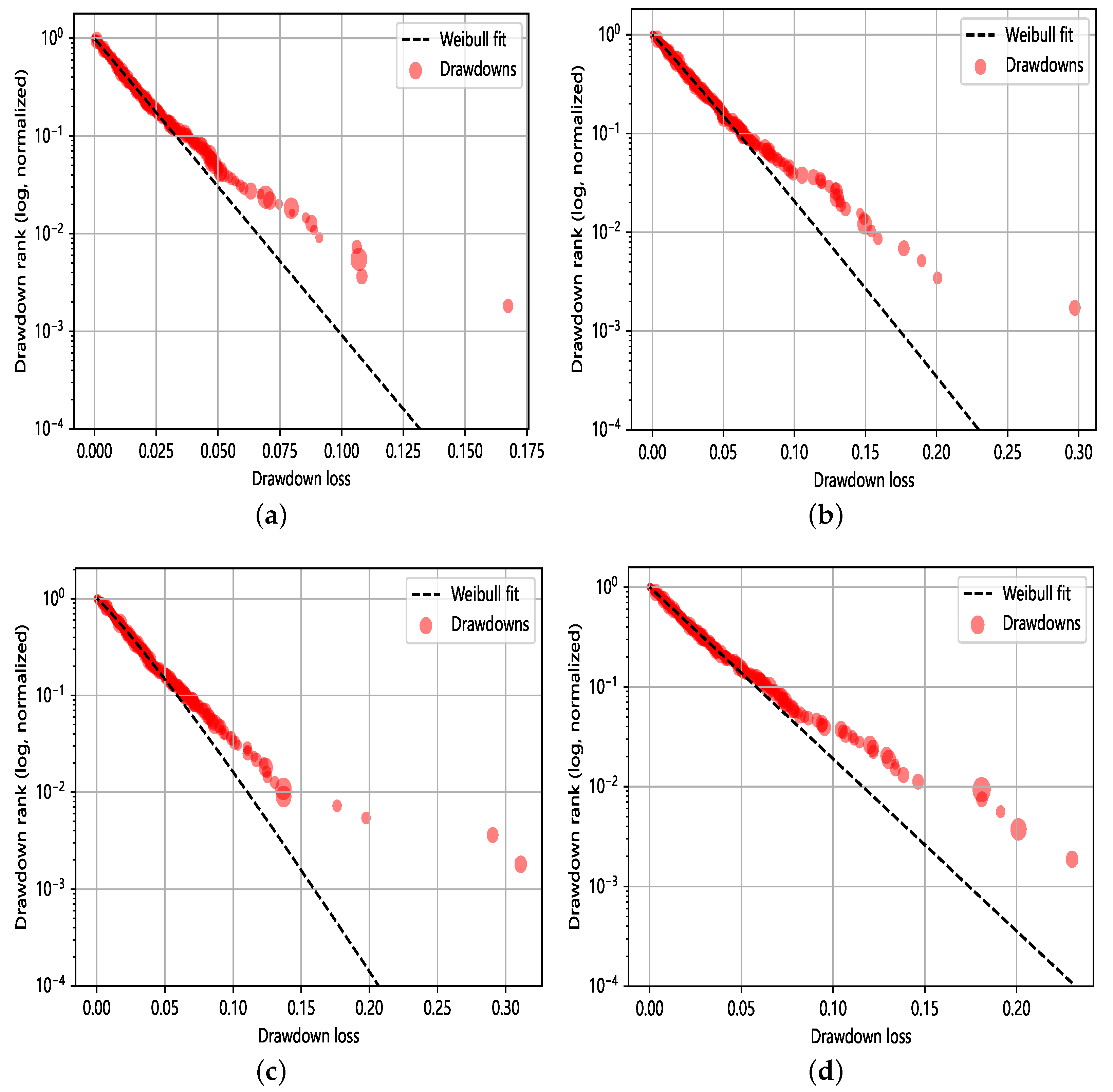
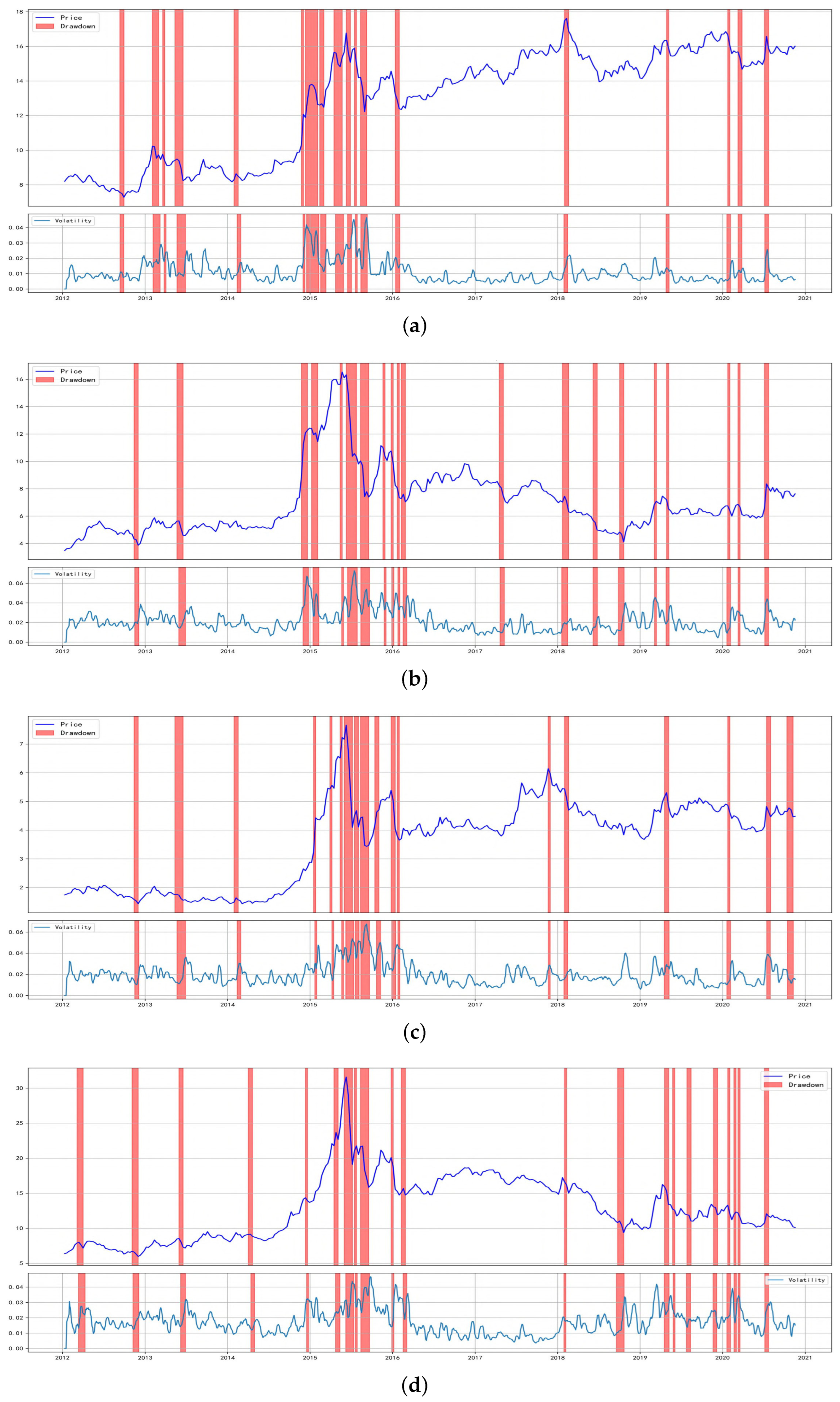
Definition and Identification of Extreme Scenarios

To investigate the characteristics of the financial sector in extreme scenarios, in this paper, the Weibull distribution model ($X\sim Weibull(\alpha ,\beta ),F\left(x\right)=1-e^{-{(x/\beta )}^{\alpha })}$) was used to fit a series of yields of financial institutions to identify extreme scenarios.

Figure 1 shows the returns for the persistent decline scenario, ranked by the size of the return. The size of the circles in the diagram corresponds to the duration of each scenario, and it can be seen that the larger retracements in the downturn scenarios did not necessarily last longer, which is consistent with the damaging and rapid outbreaks that characterize risk. Figure 1 gives a visual indication of the presence of outliers, which are defined in this paper as extreme downside scenarios.

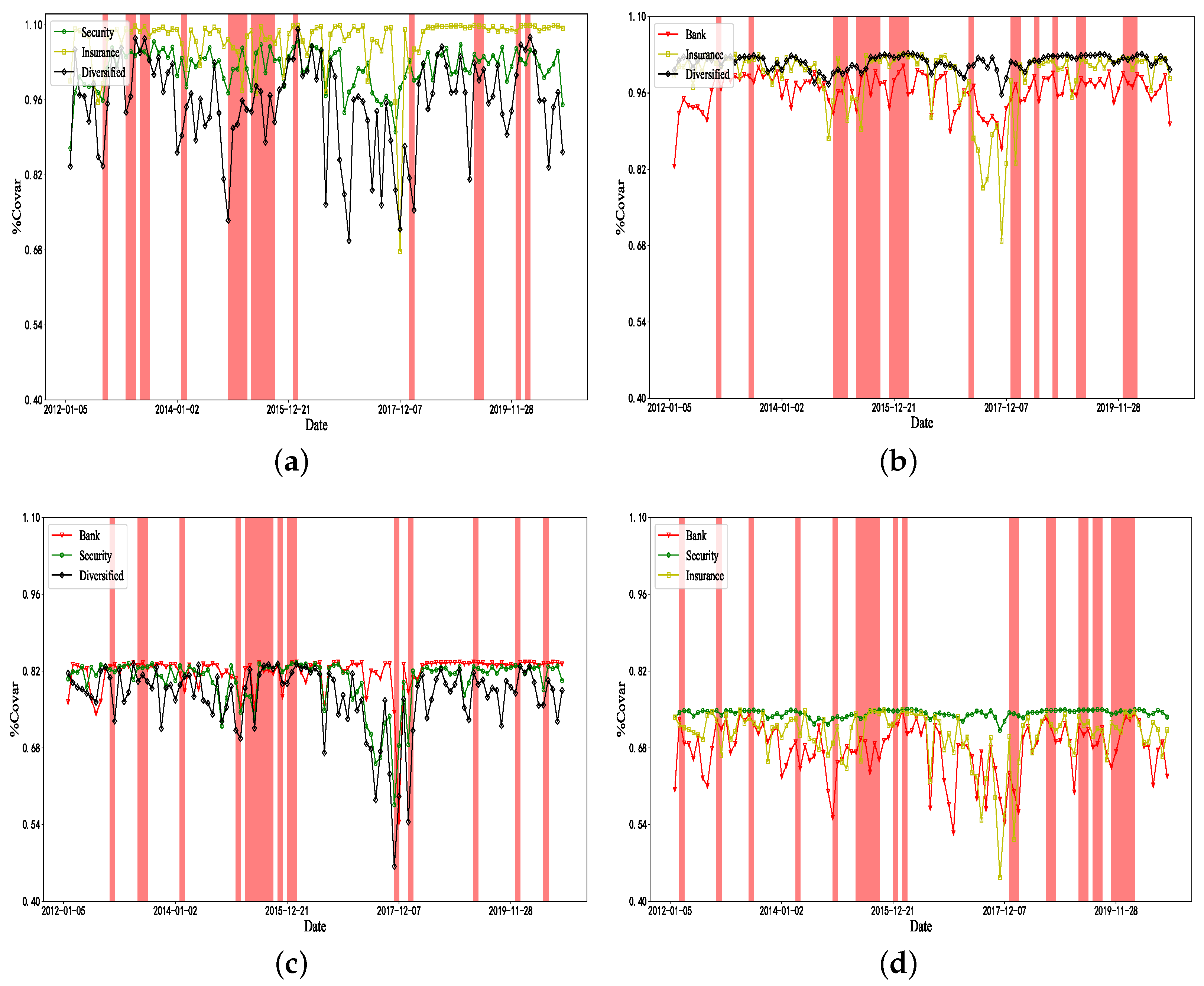
The Tail Dependence among Financial Sectors

Figure 2 shows the dynamics of the tail dependence of financial sectors. This figure shows that the trend in tail dependence was generally consistent across sectors, with a clear upward trend in extreme downturn scenarios, indicating that the tail dependence structure across financial sectors was relatively sensitive to market volatility. In particular, the tail correlations of the securities and diversified financial sectors remained consistently high following market shocks, indicating that these correlations of the securities and diversified sectors exhibited continuity from the influence of negative news, such as market declines and external crises.

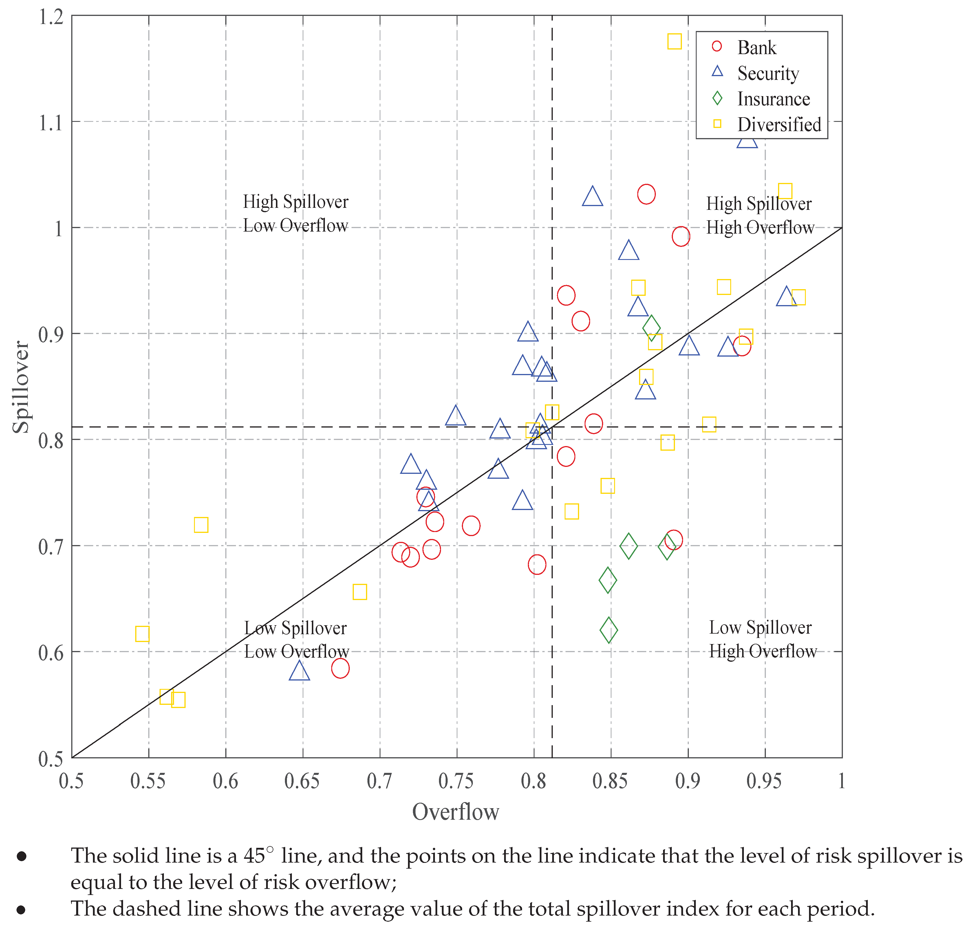
4.1.3. Financial Institution Risk Spillover Subsector Measures

Table 7. The result of risk spillover.

Full Sample Period							Extreme Scenarios
	Overflow	Banking	Securities	Insurance	Diversified	To	Banking	Securities	Insurance	Diversified	To
Spillover
Banking		0.000	1.019	1.071	0.951	3.040	0.000	1.133	1.151	1.0521	3.336
Securities		0.963	0.000	0.988	1.016	2.968	1.071	0.000	1.125	1.1281	3.324
Insurance		0.818	0.803	0.000	0.773	2.394	0.881	0.913	0.000	0.884	2.679
Diversified		0.676	0.743	0.703	0.000	2.122	0.744	0.824	0.801	0.000	2.369
From		2.458	2.565	2.762	2.740	2.631	2.696	2.871	3.077	3.065	2.927

shows the risk spillover matrix for the full sample period and the extreme scenarios, where the elements on the nonprincipal diagonal measure the directional risk spillover effect of the two interactions. The From indicator in the table indicates a sector’s exposure to aggregate risk spillovers from other sectors, with higher values indicating that the sector faces more exposure to volatility. The To indicator in the table indicates the total risk spillover from one sector to other sectors, with higher values indicating that the sector faces more exposure to volatility in the remaining sectors. In addition, the bottom-right element of each spillover matrix measures the risk spillover index of the financial system and equals the sum of all of the From or To elements.

An analysis of the overall characteristics of risk spillovers showed an asymmetry in the risk spillover relationships in the Chinese financial market, with different financial sectors playing different roles in the risk spillover process. In terms of the direction of risk absorption, the insurance and diversified financial sectors had the highest degree of risk absorption in the full sample period, reaching 2.76 and 2.74, respectively; in terms of the direction of the risk spillover, the banking and securities sectors had the most-significant risk spillover effects, reaching $3.04$ and $2.97$, respectively. This result implied that the insurance and diversified financial sectors absorbed risk spillovers, while the banking and securities sectors exported risk spillovers in the financial system. Insurance and diversified financial firms are generally seen as absorbers of risk spillovers because they are designed to take on and manage risks as a core part of their business. They are able to spread and manage risk across a large and diverse portfolio of investments. On the other hand, banks and securities firms are often seen as exporters of risk spillovers because they are more closely tied to the financial markets and are often heavily invested in securities that are susceptible to market fluctuations. Additionally, banks have a high degree of interconnectedness within the financial system, which can amplify the effects of risk spillovers. This is in line with the findings of Wang et al. [35] on the characteristics of risk spillovers among financial sectors in the U.S. In addition, in the extreme scenario, the level of risk contagion across financial institutions in all sectors increased significantly, with the total spillover coefficient increasing from $2.87$ to $2.93$.

For investors, this information suggested that investing in companies in the insurance and diversified financial sectors may provide a hedge against risk, as these sectors tend to absorb risk spillovers from other sectors. On the other hand, investing in companies in the banking and securities sectors may expose investors to increased systemic risk due to exports of risk spillovers from these sectors. For regulators, this information highlighted the need for increased oversight and regulation of the banking and securities sectors to reduce their risk-exporting behavior and prevent potential systemic risk. Regulators may also need to ensure that companies in the insurance and diversified financial sectors have sufficient risk management systems in place to effectively absorb risk spillovers. Overall, this information can inform the development of financial stability policies aimed at reducing systemic risk and promoting stability in the financial system.

Figure 3 displays the time-varying results of risk spillovers among financial sectors as a percentage of risk spillovers from one financial sector to other financial sectors. The results showed that the risk spillovers among the banking and insurance sectors, securities sector, and diversified financial sector were relatively similar throughout the sample period. This similarity can be attributed to the cross-sectoral flows of credit facilities between banks and insurance institutions, which enhance risk transmission, and the close business connections between the securities and diversified financial sectors, which lead to cross-sectoral flows of risk. In extreme downturn scenarios, external shocks result in increased risk spillovers, leading to an increase in the value at risk of the sector [2]. This result highlighted the impact of economic activity and external factors on risk transmission among financial sectors and the importance of monitoring and managing risk in these sectors. This information can be useful for investors and regulators when making informed decisions and developing strategies to mitigate risk.

The cross-sectoral risk spillover effect was highly stable in risk transmission channels between the banking and insurance sectors and between the securities and diversified financial sectors. However, in extreme situations, the risk transmission channels among other sectors can be activated, leading to an increase in the risk spillover effect. Figure 4 can further explain this relationship. The activation degree measures the proportion of the cross-sectoral risk spillover effects that are stronger than the average in the sample. In extreme scenarios, the activation of risk channels among other sectors was similar to that of the two main channels. However, as the decline weakened, there was a noticeable difference in risk transmission among sectors.

The stability in the risk transmission channels between the banking and insurance sectors and the securities and diversified financial sectors suggested that these sectors were interdependent and that the risk in one sector can easily spread to others, highlighting the importance of monitoring and managing risk in these sectors and of considering their interconnections when making investment decisions. However, in extreme situations, the activation of risk channels among other sectors can also result in an increase in the risk spillover effect, indicating that even sectors that may not typically be considered a source of risk can contribute to systemic risk. This finding highlights the need for regulators to monitor and regulate the entire financial system and to have contingency plans in place to address sudden spikes in risk.

4.1.4. Financial Institution Risk Spillover Subinstitutional Measures

To analyze the characteristics of the risk spillover of each financial institution, in this paper, a scatterplot of the level of spillover and overflow using the risk spillover index ($TI{C}^{\mathrm{To}}$) and the risk overflow index ($TI{C}^{\mathrm{From}}$) is drawn (see Figure 5). The main difference between risk spillover and risk overflow is that risk spillover is an indirect transfer of risk, while risk overflow is a direct transfer of risk.

First, financial institutions within the same sector exhibited a high level of homogeneity and similar distribution patterns. Typically, banks and securities companies were predominantly near the ${45}^{\circ }$ line of the scatterplot, but the diversified finance industry was polarized, with concentrations in both the high and low spillover and overflow areas. The insurance sector primarily operated in the high spillover-low overflow region, reflecting its inherent operational risk and impact on the overall financial system. This was due to its high level of operational complexity and diverse business model encompassing insurance, banking, and securities. For financial regulators, the distribution of each financial sector along the ${45}^{\circ }$ line provided a useful way to evaluate the stability of the financial system as a whole. Regulators should monitor firms in high spillover–high overflow regions closely, as they are more likely to experience problems that could lead to a financial crisis. On the other hand, regulators may be less concerned about firms in the low spillover–low overflow region. The concentration of the insurance sector in the high spillover–low overflow region highlighted the importance of effective regulation and supervision of the insurance sector to ensure that it does not threaten the stability of the financial system.

Second, the level of risk spillover from financial institutions was mostly clustered around the vertical dotted line, suggesting that the level of risk being transferred from one institution to another was relatively consistent across institutions. However, there was higher volatility in the level of risk overflow than in the level of risk spillover, indicating that the level of risk being transferred from one institution to another through direct transactions or financial linkages was relatively prone to fluctuations. This highlighted the need for regulators to closely monitor the level of risk overflow in the financial system to ensure that it does not threaten stability. This information may be useful for investors when evaluating the level of risk associated with different financial institutions and the stability of the financial system as a whole.

As shown in Figure 5, there was a clear sectoral echelon in the risk spillover and overflow effect, with all of the top-ranked institutions in terms of spillover and overflow intensity belonging to the diversified financial and securities sectors, suggesting that these sectors were relatively prone to rapid risk accumulation in the event of a crisis through the risk-tail-linkage process. Moreover, the risk spillover and overflow rankings of these institutions were relatively similar, suggesting that financial institutions that can spread risks to external sources also tend to have a greater ability to absorb risk. The correlation between these two risk-related capabilities may be linked to the type of business that these institutions are involved in. In the banking industry, large state-owned commercial banks are known for their stability with minimal risk spillover and overflow. This is because these government-supported banking institutions have access to timely bailouts in the case of any risks, which helps maintain their solvency and reduces overall risk. In contrast, urban commercial and joint-stock banks are more proactive in financial innovation and engage in more cutting-edge interbank transactions, which creates greater potential for risk spillover or overflow to other financial institutions.

4.2. Risk Spillover Networks for Financial Institutions

In this paper, the risk spillover matrix was filtered based on thresholds (Table 3), and the relationships among institutions were categorized into high-, moderate-, and low-risk spillovers. These relationships are presented as network diagrams.

The period from 2015 to 2017 holds specific significance as it represents the beginning and end of over-correlation in the financial market. To capture the dynamic evolution of the Chinese financial market in recent years, we evenly divided the entire period into three sub-periods. Starting from 2015, the Internet finance sector in China experienced rapid growth, witnessing the emergence of various financial services and products such as Internet monetary funds, third-party Internet payment, peer-to-peer (P2P) lending, and crowdfunding. However, this growth was accompanied by numerous failures among Internet financial platforms, leading to substantial investor losses and increased instability within the financial market. This period marked a crucial transitional stage in the financial market’s structure. Furthermore, in mid-2015, the Chinese stock market faced a period of “stock market turbulence” characterized by a widespread decline in stock prices, with thousands of stocks reaching their daily limit. This event signaled a crisis within the Chinese financial system, occurring when the overall interconnectedness among financial institutions reached its peak. At the end of 2017, China implemented stringent financial regulatory measures to address these issues. The implementation of strict scrutiny on channel business resulted in a significant reduction in cross-department collaboration, and consequently, a decline in the interconnectedness among financial institutions. These events and regulatory measures played a pivotal role in shaping the dynamics and interconnectedness of the Chinese financial market during the specified time period.

As shown in Figure 6, the high-, moderate-, and low-risk spillover networks from 2018 to 2020 are plotted from top to bottom, and the spillover networks from 2012 to 2014 and from 2015 and 2017 can be seen in Appendix A. The financial institutions were differentiated by sector, and it was discovered that the number of risk spillover connections among them varied significantly across sectors, which implied that each institution played a different role in the risk spillover network under different risk states. Moreover, the positions of the institutions in the network were found to be relatively stable over time, indicating that the risk spillover relationships among them remained consistent over time.

An examination of the high-risk spillover network diagram revealed a typical “center-edge” distribution, with the nodes corresponding to the securities sector being predominantly in the central region. However, in comparison, from 2015 to 2017 and 2018 to 2020, some joint-stock bank nodes moved toward the center and assumed a more central position in the highly risky spillover networks. The financial institution risk spillover network is a “scale-free network”, where a few nodes have more connections than do the majority of the nodes. These few highly connected financial institution nodes play a significant role in the transmission of risk and can greatly impact the stability of the network as a whole when they experience a negative impact. In the moderate- and low-risk spillover networks, there were no differences in the node distribution across sectors, with key financial sectors present in both the central and peripheral regions, but with significant intrasectoral differences. This implied that, in low- to moderate-risk conditions, each financial sector had nodes that played a crucial role in risk transmission, whereas in high-risk states, the majority of the crucial nodes for risk transmission were in the securities sector.

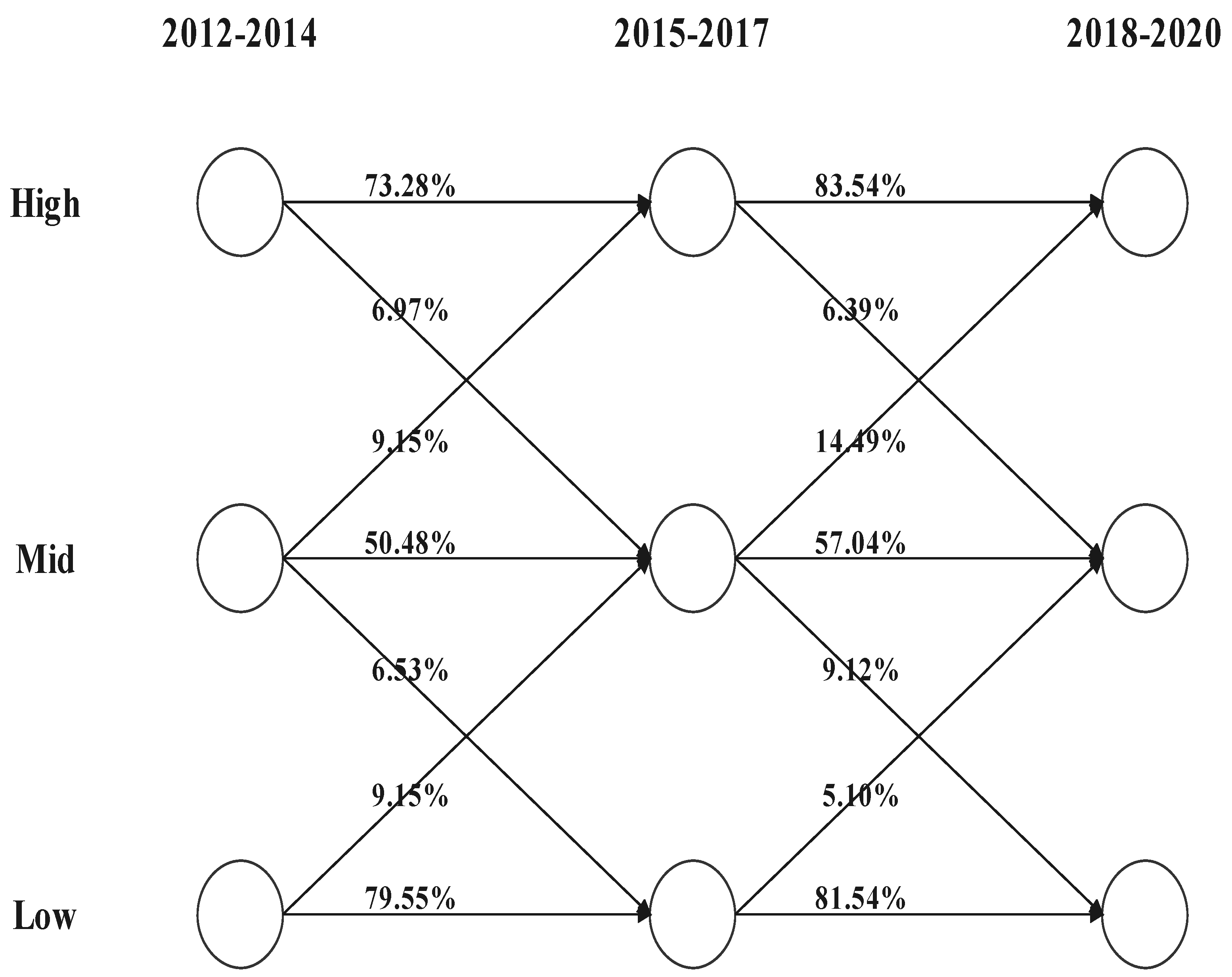
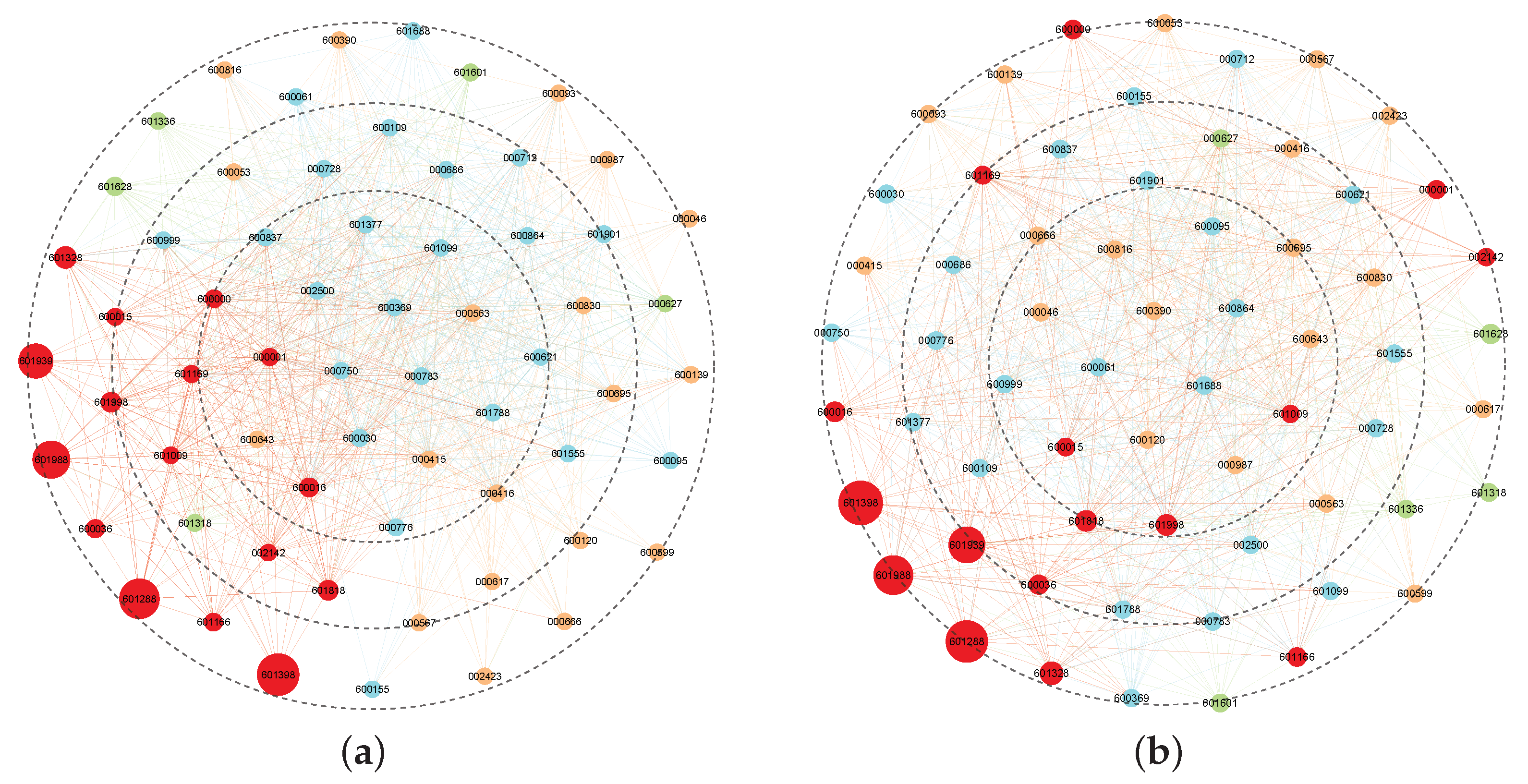
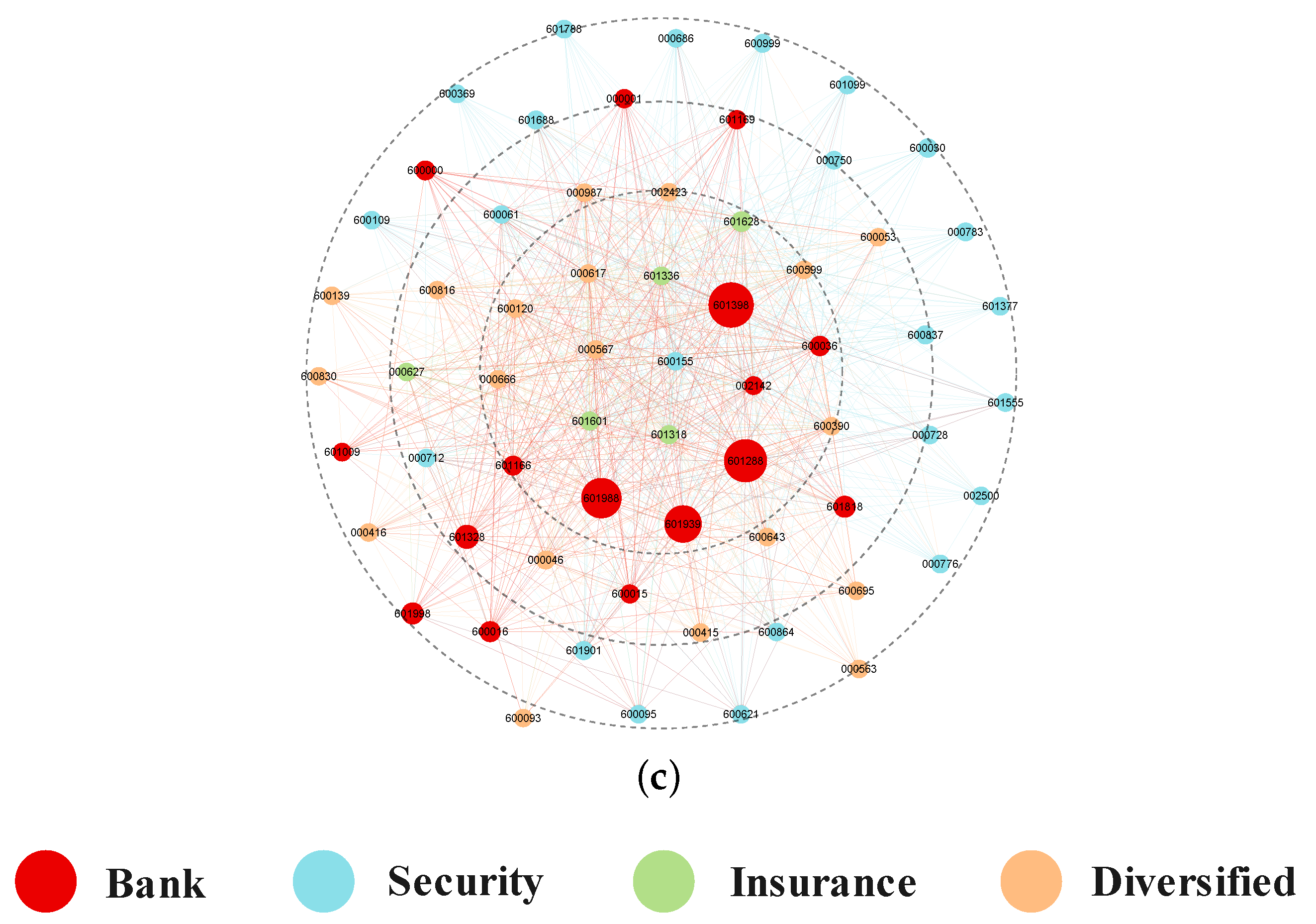
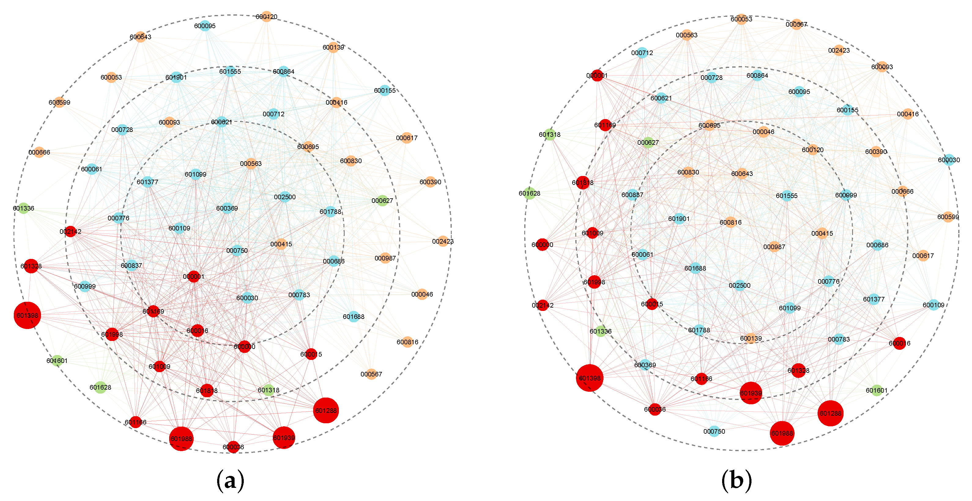
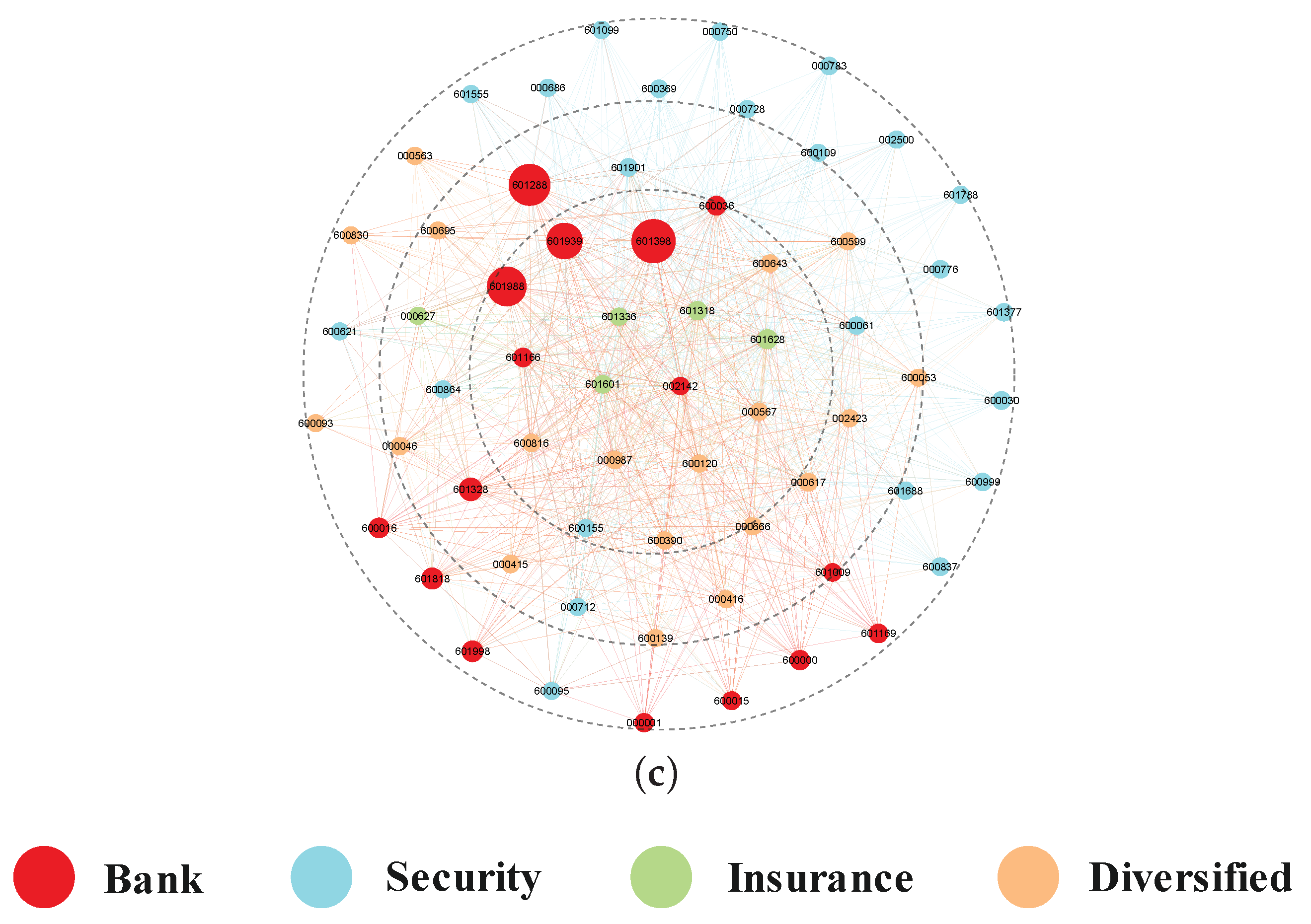
4.2.1. Evolution Analysis of Multistage Network Association Features

The correlation characteristics of the network were analyzed using four correlation indexes: density, reciprocity, aggregation coefficient, and intermediary centrality. These indexes not only reflect the extent of risk spillover correlation at different levels and stages of the network, but also reveal the hierarchical relationships within the network, providing insights into the positions of the different industries within it (Figure 7).

The network density dynamics indicated significant variability in the density of high- and low-risk spillover networks, whereas moderate-risk spillover networks featured relative stability. From 2016 to 2018, the density of high- and moderate-risk spillover networks was low, whereas the density of low-risk spillover networks was high, indicating a low level of risk spillover intensity.

The small-world effect is another metric that indicates the importance of a network. As shown in Figure 7, the aggregation coefficients demonstrated consistent changes across the three risk spillover networks, with high values and minimal variations for the high-risk spillover network. This finding indicated a strong aggregation of industry fluctuations and high transmission intensity within the high-risk spillover network and a relatively stable correlation. Conversely, reciprocity and the aggregation coefficient moved in opposite directions, implying a mutually inhibiting effect between the binary structure created by reciprocity and the ternary structure defined by the aggregation coefficient in risk spillover networks, particularly during low network density stages. Additionally, the low reciprocity of the high- and moderate-risk spillover networks suggested an asymmetric relationship among institutions, where dominant institutions had a strong impact on the risk spillover effect on other institutions. For investors, the high values and stable correlations of the aggregation coefficients in the high-risk spillover network suggested a high concentration of industry fluctuations and a high intensity of transmission effects. This may indicate not only higher risk and potentially higher returns on investments in this network, but also a greater potential for losses if the network experiences significant fluctuations. For regulators, these findings suggest a need to monitor the risk spillover effects of dominant institutions in high- and moderate-risk spillover networks, as their asymmetric relationships with other institutions may have a significant impact on the stability of the financial system. The low reciprocity in these networks highlights the potential for imbalanced risk transmission, and regulators may need to take steps to address this issue to maintain financial stability. Additionally, the mutually inhibiting effect between the binary and ternary structures in risk spillover networks, particularly at low network density stages, may also warrant regulatory attention to prevent potential systemic risks.

We analyzed the closed triads within the risk spillover networks, which consisted of single-sector, two-sector, and three-sector triads (refer to

Table 8. Risk spillover network triad in single sector.

	Triad Composition	High	Mid	Low
	Banking	187	18	5
	Securities	38	75	0
	Diversified	133	126	169
	Total	358	219	174

,

Table 9. Risk spillover network triad in two sectors.

	Triad Composition	High	Mid	Low
	Bank, Securities	1016	459	220
	Bank, Insurance	91	24	138
	Bank, Diversified	103	194	981
	Securities, Insurance	169	51	37
	Securities, Diversified	1874	1108	354
	Diversified, Insurance	14	65	315
	Total	3267	1901	2045

and

Table 10. Risk spillover network triad in three sectors.

	Triad Composition	High	Mid	Low
	Bank, Securities, Insurance	298	181	659
	Bank, Securities, Diversified	466	553	786
	Bank, Insurance, Diversified	23	83	874
	Securities, Insurance, Diversified	126	143	503
	Total	913	960	2822

for the results). The high-risk spillover network had a higher number of single-sector triads than did the moderate- or low-risk spillover networks, with a large proportion of single-sector triads consisting of the banking and diversified financial sectors. This suggested that, in high-risk states, the banking and diversified financial sectors had a strong internal risk transmission relationship. In both the high- and moderate-risk spillover networks, two-sector triads accounted for a higher share than did the other components with the securities and diversified financial sectors and the securities and banking sectors, dominating the triads. Moreover, three-sector triads were less prevalent in the high- and moderate-risk spillover networks. This implied that most of the closed-loop transmission of moderate to high risk occurred between two financial sectors rather than within a single sector or among three sectors. The results of the closed triad analysis suggested that the banking and diversified financial sectors had a strong internal risk transmission relationship in high-risk states. This highlights the potential risk of these sectors to investors, particularly during high-risk periods. Investors should closely monitor these sectors and their interactions with other sectors when evaluating their investment portfolios. The results showing that most moderate- to high-risk transmission occurred between two financial sectors highlighted the importance of monitoring and regulating the relationships among these sectors to prevent or mitigate the spread of risk. Additionally, the dominance of the securities and banking sector triad and the securities and diversified financial sector triad in both the high- and moderate-risk spillover networks suggested that regulators should focus their efforts on these sectors to prevent or mitigate the spread of risk.

Figure 8 shows the evolution of the network triad. Over 70% of the triads in the high- and low-risk spillover networks persisted to the next stage, indicating high stability. Conversely, almost half of the triads in the moderate-risk spillover network changed, with many evolving into high-risk triads. The second stage revealed a higher retention of triads at the same level and a slight improvement in the transfer of triads at different levels, suggesting that the risk spillover relationships among triads tended to stabilize during network evolution. The stability in the high- and low-risk spillover networks might indicate more predictable and stable investment opportunities for investors. However, the instability in the moderate-risk spillover network suggested that investments in these triads might be relatively risky and unpredictable. For regulators, the stability in the high- and low-risk spillover networks might imply that regulations designed to address risk spillovers in these networks could have a lasting impact. However, the relatively great instability in the moderate-risk spillover network highlighted the need for ongoing monitoring and regulation to address evolving risks in these triads.

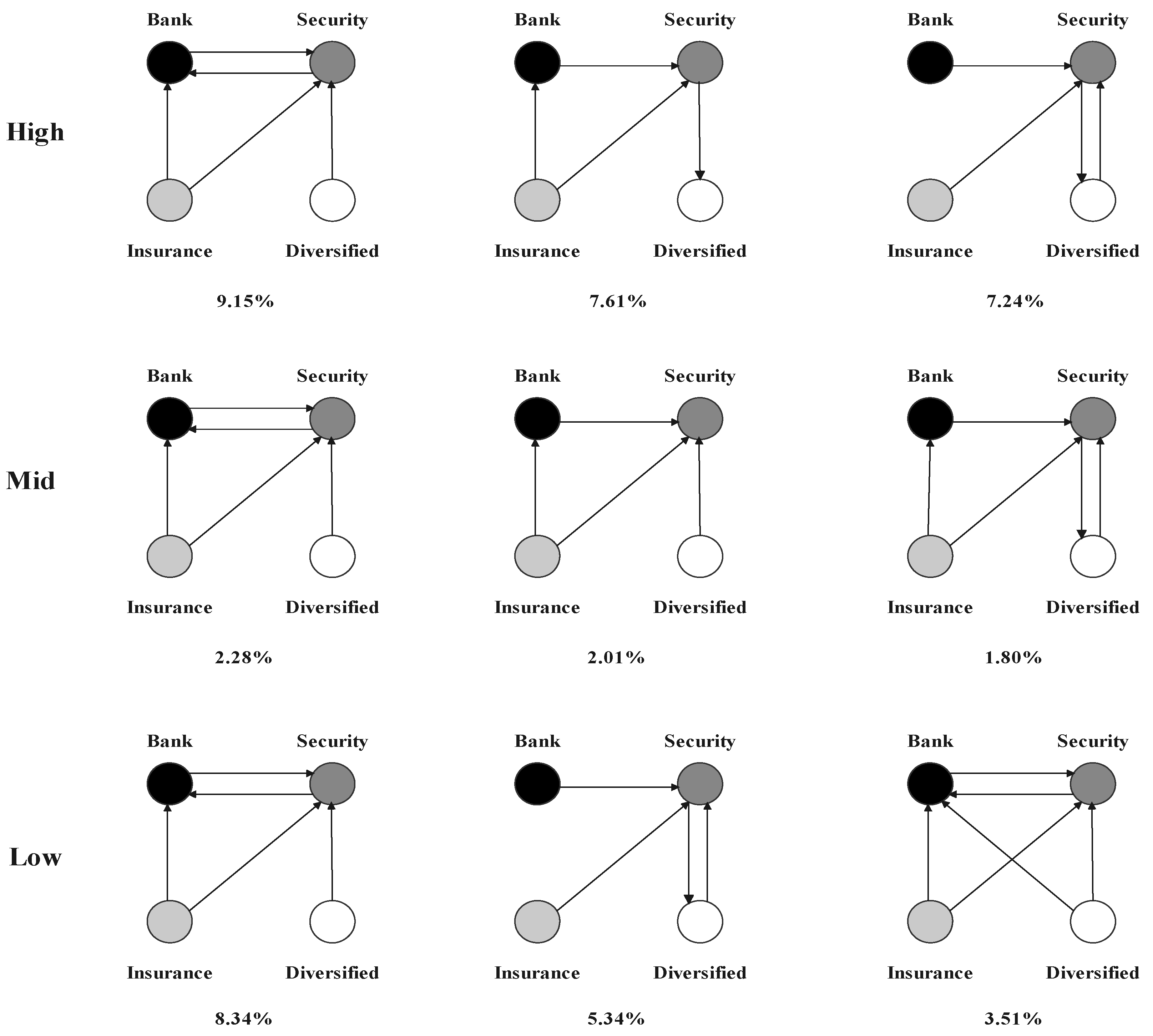
4.2.2. Motif Analysis of Risk Spillover Networks

For the risk spillover network, we conducted a network correlation analysis to identify the top three base motifs of cross-sectoral risk spillover. As shown in Figure 9, three distinct characteristics were identified at the base of the spillover network:

(1)

The securities sector was exposed to risk spillovers from all other sectors and was the primary recipient of these spillovers. Moreover, the banking and insurance sectors did not have direct risk spillover relationships with the diversified financial sectors, making the securities sector a crucial node for their risk spillovers. This implied that, in the case of a risk event, the securities sector was the first to be affected by significant risk contagion, amplifying the risk spillover effect and transmitting it to other sectors. As a result, the securities sector should be closely monitored. On the other hand, the insurance sector acted as a source of risk spillover in motifs that had significant spillovers to the banking and securities sectors.

(2)

The banking and securities sectors, as well as the securities and diversified financial sectors formed a reciprocal relationship, indicating the close transmission of risk spillovers among these three sectors. For regulators, this conclusion highlighted the need for a comprehensive and coordinated approach to monitoring and regulating these sectors. In the event of a risk event, regulators need to be aware of the potential for risk to spread quickly to other sectors and take appropriate measures to minimize the impact of such a spillover. This requires close collaboration among the different regulatory bodies responsible for each sector and a coordinated approach to mitigating potential risks.

(3)

The base motifs of the moderate- and low-risk spillover networks were comparable to those of the high-risk spillover network; however, the proportion of these motifs was significantly lower, indicating a higher concentration of base motifs in the high-risk spillover network. The base motifs with the highest proportion in the high-, moderate-, and low-risk spillover networks were the same, suggesting that these motifs revealed the most-prevalent transmission pathways for intersectoral risk spillovers. By identifying the most-common pathways for risk transmission, investors can better assess the potential impact of a risk event in one sector on other sectors and make decisions accordingly.

4.3. Study on the Mechanism of Risk Spillover Network Generation and Evolution

4.3.1. TERGM Analysis

The analysis of risk spillover networks led to the following conclusions:

(1)

Risk spillover networks had a “small-world” network topology characterized by a large number of pairwise interdependencies and a small number of highly centralized institutions that formed clusters around other institutions.

(2)

The attributes of the nodes in the network played a role in the formation of connections and preferences in the risk spillover network.

(3)

The relationships among the nodes in the network were both stable and variable over time, with coevolutionary relationships existing among different levels of risk spillover networks.

Based on these conclusions, a study of risk spillover networks was conducted through an empirical test using the TERGM to explore the endogenous mechanisms that shape the formation and evolution of risk spillover networks.

In this study, the financial institution risk spillover network was divided into yearly intervals with eight time points ranging from 2012 to 2020. The analysis focused on the moderate- and high-risk spillover networks, as the low-risk spillover network had a weak effect. The base model used for the TERGM estimation was Model (11). The results of the empirical test are presented in

Table 11. The TERGM results.

Dependent Variable:		High-Risk Spillover Network			Moderate-Risk Spillover Network
		(1)	(2)	(3)	(4)	(5)	(6)
	edges	$-0.837$ **	$-1.357$ ***	$-0.{583}^{}$	$-2.561$ ***	$-1.889$ ***	$-1.016$ **
		$\left(0.307\right)$	$\left(0.157\right)$	$\left(0.508\right)$	$\left(0.267\right)$	$\left(0.266\right)$	$\left(0.343\right)$
Structure dependent	mutual		$1.529$ ***	$1.249$ ***		$0.435$ ***	$0.505$ ***
			$\left(0.143\right)$	$\left(0.303\right)$		$\left(0.048\right)$	$\left(0.034\right)$
	gwideg		$-3.349$ ***	$-1.945$ ***		$-2.222$ ***	$-2.076$ ***
			$\left(0.268\right)$	$\left(0.216\right)$		$\left(0.197\right)$	$\left(0.253\right)$
	gwesp		$0.793$ **	$0.565$ **		$0.160$ ***	$0.145$ **
			$\left(0.139\right)$	$\left(0.138\right)$		$\left(0.042\right)$	$\left(0.044\right)$
	gwdsp		$-0.175$ ***	$-0.109$ ***		$-0.149$ ***	$-0.127$ ***
			$\left(0.011\right)$	$\left(0.021\right)$		$\left(0.014\right)$	$\left(0.007\right)$
Time- dependent	stability			$2.083$ ***			$1.167$ ***
				$\left(0.135\right)$			$\left(0.102\right)$
	variability			$0.029$ **			$0.{014}^{}$
				$\left(0.013\right)$			$\left(0.027\right)$
Sender properties	epsTTM	$-0.038$ *	$-0.036$ *	$-0.{028}^{}$	$0.023$ *	$-0.{006}^{}$	$-0.{018}^{}$
		$\left(0.020\right)$	$\left(0.018\right)$	$\left(0.020\right)$	$\left(0.013\right)$	$\left(0.013\right)$	$\left(0.013\right)$
	liability- ToAsset	$-0.341$ **	$-0.223$ *	$-0.192$ *	$0.292$ **	$0.{148}^{}$	$0.{008}^{}$
		$\left(0.127\right)$	$\left(0.13\right)$	$\left(0.112\right)$	$\left(0.128\right)$	$\left(0.130\right)$	$\left(0.166\right)$
	YOYNI	$0.029$ ***	$0.020$ *	$0.{012}^{}$	$0.{005}^{}$	$0.007$ *	$0.013$ *
		$\left(0.006\right)$	$\left(0.009\right)$	$\left(0.018\right)$	$\left(0.007\right)$	$\left(0.004\right)$	$\left(0.006\right)$
	npMargin	$0.019$ ***	$0.022$ **	$0.026$ **	$0.{008}^{}$	$-0.{002}^{}$	$0.{0003}^{}$
		$\left(0.005\right)$	$\left(0.005\right)$	$\left(0.013\right)$	$\left(0.013\right)$	$\left(0.008\right)$	$\left(0.014\right)$
Receiver properties	epsTTM	$-0.{057}^{}$	$-0.{044}^{}$	$-0.{085}^{}$	$-0.150$ *	$-0.{057}^{}$	$-0.{006}^{}$
		$\left(0.087\right)$	$\left(0.095\right)$	$\left(0.084\right)$	$\left(0.087\right)$	$\left(0.060\right)$	$\left(0.064\right)$
	liability- ToAsset	$0.860$ ***	$0.535$ **	$-0.{282}^{}$	$-0.353$ **	$-0.274$ **	$-0.{159}^{}$
		$\left(0.368\right)$	$\left(0.212\right)$	$\left(0.319\right)$	$\left(0.138\right)$	$\left(0.110\right)$	$\left(0.179\right)$
	YOYNI	$0.018$ *	$0.{014}^{}$	$0.022$ *	$0.{018}^{}$	$0.{011}^{}$	$0.{003}^{}$
		$\left(0.008\right)$	$\left(0.013\right)$	$\left(0.013\right)$	$\left(0.013\right)$	$\left(0.009\right)$	$\left(0.013\right)$
	npMargin	$-0.{001}^{}$	$0.{002}^{}$	$0.{007}^{}$	$-0.{007}^{}$	$-0.{037}^{}$	$-0.{041}^{}$
		$\left(0.024\right)$	$\left(0.019\right)$	$\left(0.019\right)$	$\left(0.041\right)$	$\left(0.043\right)$	$\left(0.047\right)$
Sectoral properties	industry	$0.162$ **	$0.168$ ***	$0.167$ ***	$-0.{053}^{}$	$-0.092$ *	$-0.{025}^{}$
		$\left(0.052\right)$	$\left(0.027\right)$	$\left(0.026\right)$	$\left(0.061\right)$	$\left(0.045\right)$	$\left(0.070\right)$
Coevolutionary properties	high-risk spillover network				$1.706$ ***	$1.513$ ***	$0.676$ ***
					$\left(0.083\right)$	$\left(0.079\right)$	$\left(0.164\right)$
	moderate-risk spillover network	$3.738$ ***	$3.201$ ***	$1.222$ **
		$\left(0.402\right)$	$\left(0.313\right)$	$\left(0.424\right)$
	low-risk spillover network	$-7.273$ **	$-5.031$ *	$-2.616$ ***	$-3.397$ ***	$-2.688$ ***	$-2.501$ ***
		$\left(2.864\right)$	$\left(2.341\right)$	$\left(0.667\right)$	$\left(0.516\right)$	$\left(0.561\right)$	$\left(0.607\right)$

* p < 0.1; ** p < 0.05; *** p < 0.01.

. Six regressions were run, with Regressions (1) and (4) including only exogenous mechanism variables and Regressions (2) and (5), (3), and (6) including variables for structure- and time-dependent effects, respectively, to examine the endogenous mechanism of the network. The final model estimated the parameters of the various effects, representing the frequency at which the corresponding network structure appeared in the network.

The results of the regressions in Groups (3) and (6) provided strong evidence that supported Hypothesis 1, which posits that reciprocity has a positive impact on the formation of both high- and moderate-risk spillover networks. This was demonstrated by the significant and positive coefficients of reciprocity (${\theta }_1$), which had a value of 1.249 in Group (3) and 0.505 in Group (6). These findings suggested that the presence of reciprocal connections led to the development of stronger risk spillover relationships among financial institutions and a greater number of two-way connections. The magnitude of the coefficients indicated that the reciprocal effect was more pronounced in high-risk than in moderate-risk spillover networks. Additionally, the results supported Hypothesis 2, which states that the degree of nodes in highly risky spillover networks is not uniformly distributed. This was evidenced by the significant and negative coefficients of convergence (${\theta }_2$), which had values of −1.945 in Group (3) and −2.076 in Group (6). The negative coefficients indicated that a small number of financial institutions were more vulnerable to risk spillovers and, thus, evolved into central nodes within the network. These findings demonstrated the importance of considering the network structure in the analysis of risk spillover dynamics among financial institutions. The results of the regressions in Groups (2) and (5) highlighted the interplay between convergence and time-dependent effects on the formation of risk spillover relationships. The partially offsetting effect of convergence was reflected in a comparison of the convergence coefficients in these regressions, showcasing the complexity of risk spillover dynamics. Furthermore, the significant coefficients of transmittance (${\theta }_3$) in Regressions (3) and (6) with values of 0.565 and 0.145, respectively, provided evidence for the existence of a transmission effect in the risk spillover network. This suggests that financial institutions tend to form closed triads, making the risk spillover relationship more communicative. The significant coefficient supports the validity of Hypothesis 3, indicating the presence of a transmission effect in the risk spillover network. Additionally, the significant and negative connectivity coefficient (${\theta }_4$) of −0.109 in Group (3) and the positive coefficient of 0.127 in Group (6) suggested that the risk spillover network had connectivity and the potential for multiple-path propagation. This highlighted the importance of considering network connectivity in the analysis of risk spillover dynamics among financial institutions. Finally, the largest parameter estimate among the structural variables was the convergence coefficient (${\theta }_2$), which suggested that convergence had the greatest impact on the formation and evolution of risk spillover relationships among financial institutions.

The significant stability coefficients (${\theta }_6$) in Regressions (3) and (6), with values of 2.083 and 1.167, respectively, indicated that the risk spillover networks had some degree of stability over time. This suggested that the risk spillover relationships among financial institutions tended to persist, with higher-risk spillover networks being more stable. The significant stability coefficients provided evidence to support Hypothesis 5, which posits that the risk spillover networks are stable. Additionally, the coefficient of variability (${\theta }_7$) in Regression (3) with a value of 0.014 was significant, indicating that the time effect had a dampening impact on the relationship generation and evolution of the high-risk spillover network. This suggested that the risk spillover relationship tended to fade away over time. In contrast, the coefficient of variability (${\theta }_7$) in Regression (6) was not significant, which meant that Hypothesis 6 cannot be tested for moderate-risk spillover networks. This lack of significance may indicate that the time effect did not have a significant impact on the formation or evolution of moderate-risk spillover networks.

The results of the study revealed that, as structural and time-dependent effects were incorporated into the model, the influence of exogenous mechanisms appeared to decline, and some variables underwent a change in significance. For instance, the sender attribute (epsTTM) coefficient increased from −0.038 to −0.028. This change highlighted the impact of the additional effects on the sender attribute’s significance. Additionally, this study showed that the coefficients of the structural dependence variables in Regression Group (3) were lower than those of Regression Group (2), demonstrating the partially offsetting effect of structural dependence on a highly risky spillover network under the influence of the time dependence effect. This observation highlighted the interplay between structural and time-dependent effects on the formation and evolution of risk spillover networks. The decrease in the coefficients of the structural dependence variables suggested that the effect of structural dependence was less pronounced when the time-dependent effect was considered.

Industry homogeneity gauges the likelihood that financial institutions in the same sector form risk spillover relationships. The results of Regression Group (3) revealed a positive coefficient $thet{a}_8$ of homogeneity, demonstrating that financial institutions were inclined to establish high-risk spillover relationships with others in the same sector, as previously analyzed. Additionally, the high-risk spillover network’s coefficient for the evolution of the moderate-risk spillover network relationship was positive and significant, indicating that the moderate-risk spillover network’s spillover relationship in the preceding period amplified the formation of its high-risk spillover relationship in the following period. On the other hand, the coefficient $thet{a}_8$ of homogeneity in Regression Group (6) was not significant, indicating a lack of sectoral preference in the connections in the moderate-risk spillover network. The positive and significant coefficient of the evolution of the high-risk spillover relationship in this case showed that the high-risk spillover network’s spillover relationship from the previous period affected the formation of the moderate-risk spillover relationship in the next period, suggesting a symbiotic and mutually reinforcing relationship between the high- and moderate-risk spillover network.

In conclusion, this paper’s empirical findings suggested that the formation and progression of risk spillover networks were influenced by a mixture of external and internal factors. Among these factors, the structural and time-related effects within internal mechanisms hold relatively great explanatory power for the formation and development of these networks.

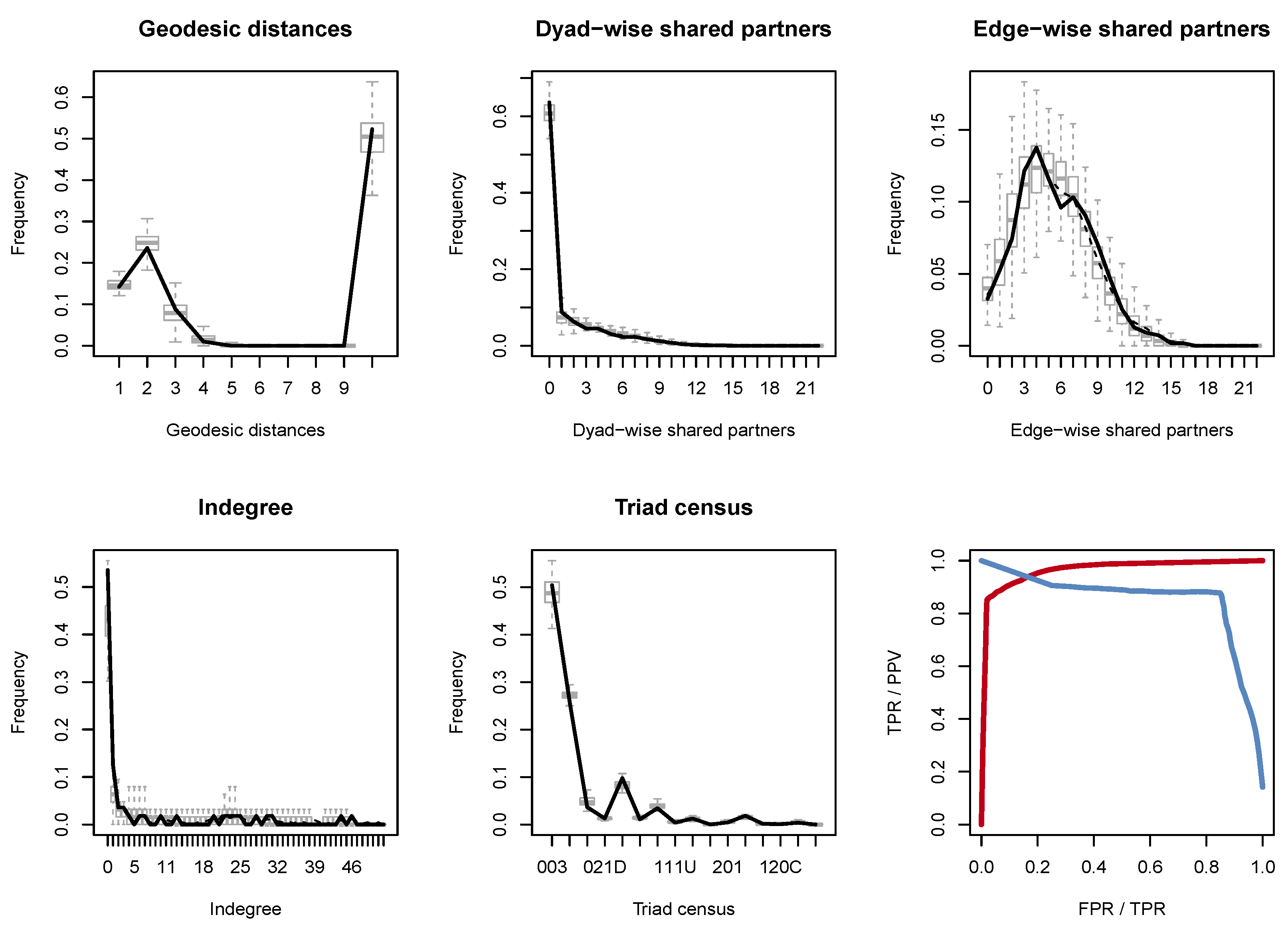
4.3.2. Goodness-of-Fit Test

In this paper, the fit of the TERGM was assessed using a model simulation-based goodness-of-fit evaluation method. One thousand networks were simulated based on Model 3, as shown in Figure 10, with the solid black line representing real network metrics and the box plot representing the 95% confidence interval of the simulated network metrics. The results showed that key network features, such as indegree, gwesp, gwdsp, triad census, and geodesic distance, were within the 95% confidence interval of the simulated network, indicating a close fit between the simulated and real networks and suggesting that the TERGM accurately captured the endogenous generation mechanism of the real network.

5. Conclusions

The development of financial markets leads to increased complexity and risk spillovers among institutions. This study constructed a risk spillover network based on the CoVaR estimates. This network represented the relationships and interactions among financial institutions in terms of risk spillover. Each institution was considered a node in the network, and the connections between nodes represented the strength and direction of risk transmission. The study examined the characteristics of the risk spillover network, including the degree of interconnectedness, the centrality of institutions, and the overall structure of the network. It also analyzed the risk transmission paths within the network, identifying how risks propagate from one institution to another. To gain a comprehensive understanding of the network, the study investigated the dynamic evolution of the risk spillover network under different risk states. This analysis allowed for an examination of how the network’s structure and risk transmission patterns changed during different market conditions or periods of heightened risk.

The empirical results suggested the following. First, financial institutions play different roles in the risk spillover process, with the securities and banking sectors being risk exporters and the insurance and diversified financial sectors being risk takers. The closest risk spillover relationships existed between the banking and insurance sectors and between the securities and diversified financial sectors. The conclusion highlighted that the securities and banking sectors are risk exporters. This finding is in line with the understanding that investment banks and other securities firms, as well as commercial banks often have significant exposures to various financial instruments and markets. Their interconnectedness and the potential for fire sales or contagion effects can contribute to the transmission of risks across the system. Likewise, the identification of the insurance and diversified financial sectors as risk takers suggested that these sectors might be more susceptible to absorbing risks from other parts of the financial system. Insurance companies, for instance, may face risks related to underwriting, investment activities, and exposure to catastrophic events. Diversified financial institutions, such as conglomerates or financial holding companies, typically have diverse business lines and may have exposures across multiple sectors.

Second, there is a significant amount of intrasectoral risk transmission between banks and the diversified financial sector in high-risk situations, as well as dual-sectoral risk contagion between banks and the securities sector, with transmission between the diversified financial and securities sectors being the most-common; moreover, risk transmission across multiple sectors existed to a lesser extent. The conclusion’s finding of significant intrasectoral risk transmission between banks and the diversified financial sector aligns with previous research indicating that risks can propagate within a particular sector. Financial institutions within the same sector often share similar exposures, interconnectedness, and risk profiles, which can lead to the transmission of risks among them. In high-risk situations, such intrasectoral risk transmission becomes more prominent. The observation of dual-sectoral risk contagion between banks and the securities sector suggests that risks can flow between these two sectors in a mutually reinforcing manner. This finding is consistent with the understanding that banks and securities firms often have interconnected activities and exposures, such as lending, trading, and investments in securities. During periods of stress or high-risk events, adverse developments in one sector can amplify risks in the other, leading to dual-sectoral risk contagion. The conclusion highlights that transmission between the diversified financial and securities sectors is the most-common. This implies that risks are particularly prone to flow between these two sectors. This aligns with the understanding that diversified financial institutions often have exposures across various sectors and may engage in activities similar to securities firms, such as investment banking or asset management. Therefore, the interconnectedness between diversified financial and securities sectors can facilitate risk transmission.

Finally, the securities sector serves as the pivotal node for risk spillovers, transmitting intersectoral risks. The formation and evolution of risk spillover networks are influenced by endogenous mechanisms, with the convergence effect being the most-notable. This study found coevolutionary relationships for different degrees of spillover networks.

The conclusion’s finding that the securities sector serves as the pivotal node for risk spillovers aligns with previous research on systemic risk and interconnectedness in financial systems. The securities sector, which includes investment banks, brokerage firms, and exchanges, often plays a crucial role in facilitating the flow of capital and financial transactions. Consequently, it can serve as a key channel for the transmission of risks across different sectors of the financial system. The notion that the formation and evolution of risk spillover networks are influenced by endogenous mechanisms is also consistent with previous research. Endogenous mechanisms refer to the internal dynamics and interactions among financial institutions that shape the transmission of risks. These mechanisms can include interconnectedness, contagion effects, feedback loops, and the behavior of market participants. The conclusion suggested that the convergence effect, which refers to the tendency of risks to converge towards specific nodes or sectors, is particularly notable in influencing the risk spillover networks. Furthermore, the mention of coevolutionary relationships in different degrees of spillover networks implied that the characteristics and dynamics of the risk spillover networks are not static. Coevolutionary relationships suggested that the network structure and the behavior of institutions within the network influence each other in an interconnected manner. This finding aligns with the understanding that the interconnectedness and behavior of financial institutions can evolve over time, leading to changes in the patterns and strength of risk transmission.

Overall, using the Copula-CoVaR to analyze risk spillover relationships and dynamics within and across the four sectors of banking, securities, insurance, and diversified finance and examining the mechanisms for the generation and evolution of risk spillover networks are important to understanding risk spillovers and financial sector linkages in China’s financial markets.

To prevent intersectoral overdependence, regulators can take several measures to address the complexities and risks in the financial system. Firstly, they should formulate policies that account for the specific characteristics and vulnerabilities of each major financial sector, promoting resilience within each sector. Additionally, adopting a risk-based approach to regulation enables regulators to identify and monitor intersectoral risks, facilitating the formulation of targeted and effective regulatory measures. Strengthening supervisory frameworks and monitoring systems allows regulators to assess and manage intersectoral risks by regularly evaluating the risk exposure and interconnectedness of financial institutions. Lastly, fostering collaboration and information sharing among regulatory authorities responsible for different sectors enhances the understanding of intersectoral risks, improves coordination during crises, and supports the development of a stable network of polycentric nodes. These measures collectively contribute to a more robust and resilient financial system.

References

1. Acharya, V.V.; Pedersen, L.H.; Philippon, T.; Richardson, M. Measuring Systemic Risk. Rev. Financ. Stud. 2016, 30, 2–47. [Google Scholar] [CrossRef] [Green Version]
2. Adams, Z.; Füss, R.; Gropp, R. Spillover Effects among Financial Institutions: A State-Dependent Sensitivity Value-at-Risk Approach. J. Financ. Quant. Anal. 2014, 49, 575–598. [Google Scholar] [CrossRef] [Green Version]
3. Hautsch, N.; Schaumburg, J.; Schienle, M. Financial Network Systemic Risk Contributions. Rev. Financ. 2014, 19, 685–738. [Google Scholar] [CrossRef] [Green Version]
4. Tobias, A.; Brunnermeier, M.K. CoVaR. Am. Econ. Rev. 2016, 106, 1705–1741. [Google Scholar]
5. Girardi, G.; Tolga Ergün, A. Systemic risk measurement: Multivariate GARCH estimation of CoVaR. J. Bank. Financ. 2013, 37, 3169–3180. [Google Scholar] [CrossRef]
6. Jin, X. Downside and upside risk spillovers from China to Asian stock markets: A CoVaR-Copula approach. Financ. Res. Lett. 2018, 25, 202–212. [Google Scholar] [CrossRef]
7. Jian, Z.; Wu, S.; Zhu, Z. Asymmetric extreme risk spillovers between the Chinese stock market and index futures market: An MV-CAViaR based intraday CoVaR approach. Emerg. Mark. Rev. 2018, 37, 98–113. [Google Scholar] [CrossRef]
8. Bellavite Pellegrini, C.; Cincinelli, P.; Meoli, M.; Urga, G. The role of shadow banking in systemic risk in the European financial system. J. Bank. Financ. 2022, 138, 106422. [Google Scholar] [CrossRef]
9. Acharya, V.; Engle, R.; Richardson, M. Capital Shortfall: A New Approach to Ranking and Regulating Systemic Risks. Am. Econ. Rev. 2012, 102, 59–64. [Google Scholar] [CrossRef] [Green Version]
10. Brownlees, C.; Engle, R.F. SRISK: A Conditional Capital Shortfall Measure of Systemic Risk. Rev. Financ. Stud. 2016, 30, 48–79. [Google Scholar] [CrossRef] [Green Version]
11. Bellavite Pellegrini, C.; Cincinelli, P.; Meoli, M.; Urga, G. The contribution of (shadow) banks and real estate to systemic risk in China. J. Financ. Stab. 2022, 60, 101018. [Google Scholar] [CrossRef]
12. Wang, G.J.; Jiang, Z.Q.; Lin, M.; Xie, C.; Stanley, H.E. Interconnectedness and systemic risk of China’s financial institutions. Emerg. Mark. Rev. 2018, 35, 1–18. [Google Scholar] [CrossRef]
13. Ji, Q.; Liu, B.Y.; Nehler, H.; Uddin, G.S. Uncertainties and extreme risk spillover in the energy markets: A time-varying Copula-based CoVaR approach. Energy Econ. 2018, 76, 115–126. [Google Scholar] [CrossRef]
14. Gong, X.L.; Liu, X.H.; Xiong, X.; Zhang, W. Financial systemic risk measurement based on causal network connectedness analysis. Int. Rev. Econ. Financ. 2019, 64, 290–307. [Google Scholar] [CrossRef]
15. Minoiu, C.; Reyes, J.A. A network analysis of global banking: 1978–2010. J. Financ. Stab. 2013, 9, 168–184. [Google Scholar] [CrossRef]
16. Georg, C.P. The effect of the interbank network structure on contagion and common shocks. J. Bank. Financ. 2013, 37, 2216–2228. [Google Scholar] [CrossRef] [Green Version]
17. Benoit, S.; Colliard, J.E.; Hurlin, C.; Pérignon, C. Where the Risks Lie: A Survey on Systemic Risk. Rev. Financ. 2016, 21, 109–152. [Google Scholar] [CrossRef]
18. Wang, Y.; Li, H.; Guan, J.; Liu, N. Similarities between stock price correlation networks and co-main product networks: Threshold scenarios. Phys. A Stat. Mech. Its Appl. 2019, 516, 66–77. [Google Scholar] [CrossRef]
19. Yang, C.; Zhu, X.; Li, Q.; Chen, Y.; Deng, Q. Research on the evolution of stock correlation based on maximal spanning trees. Phys. A Stat. Mech. Its Appl. 2014, 415, 1–18. [Google Scholar] [CrossRef]
20. Barbi, A.; Prataviera, G. Nonlinear dependencies on Brazilian equity network from mutual information minimum spanning trees. Phys. A Stat. Mech. Its Appl. 2019, 523, 876–885. [Google Scholar] [CrossRef] [Green Version]
21. Diebold, F.X.; Yılmaz, K. On the network topology of variance decompositions: Measuring the connectedness of financial firms. J. Econom. 2014, 182, 119–134. [Google Scholar] [CrossRef] [Green Version]
22. Lundgren, A.I.; Milicevic, A.; Uddin, G.S.; Kang, S.H. Connectedness network and dependence structure mechanism in green investments. Energy Econ. 2018, 72, 145–153. [Google Scholar] [CrossRef]
23. Zeng, T.; Yang, M.; Shen, Y. Fancy Bitcoin and conventional financial assets: Measuring market integration based on connectedness networks. Econ. Model. 2020, 90, 209–220. [Google Scholar] [CrossRef]
24. Ji, Q.; Bouri, E.; Lau, C.K.M.; Roubaud, D. Dynamic connectedness and integration in cryptocurrency markets. Int. Rev. Financ. Anal. 2019, 63, 257–272. [Google Scholar] [CrossRef]
25. Härdle, W.K.; Wang, W.; Yu, L. TENET: Tail-Event driven NETwork risk. J. Econom. 2016, 192, 499–513. [Google Scholar] [CrossRef]
26. Liu, B.Y.; Fan, Y.; Ji, Q.; Hussain, N. High-dimensional CoVaR network connectedness for measuring conditional financial contagion and risk spillovers from oil markets to the G20 stock system. Energy Econ. 2022, 105, 105749. [Google Scholar] [CrossRef]
27. Chen, L.; Han, Q.; Qiao, Z.; Stanley, H.E. Correlation analysis and systemic risk measurement of regional, financial and global stock indices. Phys. A Stat. Mech. Its Appl. 2020, 542, 122653. [Google Scholar] [CrossRef]
28. Silva, T.C.; Guerra, S.M.; Tabak, B.M.; de Castro Miranda, R.C. Financial networks, bank efficiency and risk-taking. J. Financ. Stab. 2016, 25, 247–257. [Google Scholar] [CrossRef]
29. Poledna, S.; Bochmann, O.; Thurner, S. Basel III capital surcharges for G-SIBs are far less effective in managing systemic risk in comparison to network-based, systemic risk-dependent financial transaction taxes. J. Econ. Dyn. Control 2017, 77, 230–246. [Google Scholar] [CrossRef] [Green Version]
30. Sun, Q.; Gao, X.; Wen, S.; Chen, Z.; Hao, X. The transmission of fluctuation among price indices based on Granger causality network. Phys. A Stat. Mech. Its Appl. 2018, 506, 36–49. [Google Scholar] [CrossRef]
31. Ji, Q.; Bouri, E.; Roubaud, D. Dynamic network of implied volatility transmission among US equities, strategic commodities, and BRICS equities. Int. Rev. Financ. Anal. 2018, 57, 1–12. [Google Scholar] [CrossRef]
32. Yun, T.S.; Jeong, D.; Park, S. “Too central to fail” systemic risk measure using PageRank algorithm. J. Econ. Behav. Organ. 2019, 162, 251–272. [Google Scholar] [CrossRef]
33. Li, S.; Liu, M.; Wang, L.; Yang, K. Bank multiplex networks and systemic risk. Phys. A Stat. Mech. Its Appl. 2019, 533, 122039. [Google Scholar] [CrossRef]
34. Billio, M.; Getmansky, M.; Lo, A.W.; Pelizzon, L. Econometric measures of connectedness and systemic risk in the finance and insurance sectors. J. Financ. Econ. 2012, 104, 535–559. [Google Scholar] [CrossRef]
35. Wang, G.J.; Xie, C.; He, K.; Stanley, H. Extreme risk spillover network: Application to financial institutions. Quant. Financ. 2017, 17, 1417–1433. [Google Scholar] [CrossRef]
36. Karimalis, E.N.; Nomikos, N.K. Measuring systemic risk in the European banking sector: A Copula CoVaR approach. Eur. J. Financ. 2018, 24, 944–975. [Google Scholar] [CrossRef] [Green Version]
37. Drakos, A.A.; Kouretas, G.P. Bank ownership, financial segments and the measurement of systemic risk: An application of CoVaR. Int. Rev. Econ. Financ. 2015, 40, 127–140. [Google Scholar] [CrossRef]
38. Bernard, C.; Czado, C. Conditional quantiles and tail dependence. J. Multivar. Anal. 2015, 138, 104–126. [Google Scholar] [CrossRef]
39. Trabelsi, N.; Naifar, N. Are Islamic stock indexes exposed to systemic risk? Multivariate GARCH estimation of CoVaR. Res. Int. Bus. Financ. 2017, 42, 727–744. [Google Scholar] [CrossRef]
40. Fang, L.; Chen, B.; Yu, H.; Qian, Y. Identifying systemic important markets from a global perspective: Using the ADCC ΔCoVaR approach with skewed-t distribution. Financ. Res. Lett. 2018, 24, 137–144. [Google Scholar] [CrossRef]
41. Bernardi, M.; Durante, F.; Jaworski, P. CoVaR of families of Copulas. Stat. Probab. Lett. 2017, 120, 8–17. [Google Scholar] [CrossRef]
42. Kayalar, D.E.; Küçüközmen, C.C.; Selcuk-Kestel, A.S. The impact of crude oil prices on financial market indicators: Copula approach. Energy Econ. 2017, 61, 162–173. [Google Scholar] [CrossRef]
43. Talbi, M.; de Peretti, C.; Belkacem, L. Dynamics and causality in distribution between spot and future precious metals: A Copula approach. Resour. Policy 2020, 66, 101645. [Google Scholar] [CrossRef]
44. Abakah, E.J.A.; Addo, E.; Gil-Alana, L.A.; Tiwari, A.K. Re-examination of international bond market dependence: Evidence from a pair Copula approach. Int. Rev. Financ. Anal. 2021, 74, 101678. [Google Scholar] [CrossRef]
45. Patton, A.J. Modelling Asymmetric Exchange Rate Dependence. Int. Econ. Rev. 2006, 47, 527–556. [Google Scholar] [CrossRef] [Green Version]
46. Chen, W.; Wei, Y.; Zhang, B.; Yu, J. Quantitative measurement of the contagion effect between US and Chinese stock market during the financial crisis. Phys. A Stat. Mech. Its Appl. 2014, 410, 550–560. [Google Scholar] [CrossRef]
47. Martinez-Jaramillo, S.; Alexandrova-Kabadjova, B.; Bravo-Benitez, B.; Solórzano-Margain, J.P. An empirical study of the Mexican banking system’s network and its implications for systemic risk. J. Econ. Dyn. Control 2014, 40, 242–265. [Google Scholar] [CrossRef]
48. Huang, W.Q.; Zhuang, X.T.; Yao, S.; Uryasev, S. A financial network perspective of financial institutions’ systemic risk contributions. Phys. A Stat. Mech. Its Appl. 2016, 456, 183–196. [Google Scholar] [CrossRef]
49. Lusher, D.; Koskinen, J.; Robins, G. Exponential Random Graph Models for Social Networks: Theory, Methods, and Applications; Cambridge University Press: Cambridge, UK, 2013. [Google Scholar]
50. Pircalabelu, E.; Claeskens, G. Focused model selection for social networks. Soc. Netw. 2016, 46, 76–86. [Google Scholar] [CrossRef] [Green Version]
51. Yu, G.; Xiong, C.; Xiao, J.; He, D.; Peng, G. Evolutionary analysis of the global rare earth trade networks. Appl. Math. Comput. 2022, 430, 127249. [Google Scholar] [CrossRef]
52. Obando, C.; Rosso, C.; Siegel, J.; Corbetta, M.; De Vico Fallani, F. Temporal exponential random graph models of longitudinal brain networks after stroke. J. R. Soc. Interface 2022, 19, 20210850. [Google Scholar] [CrossRef] [PubMed]
53. Yin, M.; Zhu, L. Reciprocity in directed networks. Phys. A Stat. Mech. Its Appl. 2016, 447, 71–84. [Google Scholar] [CrossRef] [Green Version]
54. Garlaschelli, D.; Loffredo, M.I. Patterns of Link Reciprocity in Directed Networks. Phys. Rev. Lett. 2004, 93, 268701. [Google Scholar] [CrossRef] [Green Version]
55. Drehmann, M.; Tarashev, N. Measuring the systemic importance of interconnected banks. J. Financ. Intermediat. 2013, 22, 586–607. [Google Scholar] [CrossRef] [Green Version]
56. Barabási, A.L.; Albert, R. Emergence of Scaling in Random Networks. Science 1999, 286, 509–512. [Google Scholar] [CrossRef] [PubMed] [Green Version]
57. Battiston, S.; Delli Gatti, D.; Gallegati, M.; Greenwald, B.; Stiglitz, J.E. Liaisons dangereuses: Increasing connectivity, risk sharing, and systemic risk. J. Econ. Dyn. Control 2012, 36, 1121–1141. [Google Scholar] [CrossRef] [Green Version]
58. Giuliani, E. Network dynamics in regional clusters: Evidence from Chile. Res. Policy 2013, 42, 1406–1419. [Google Scholar] [CrossRef]
59. Guo, H.; Sun, Y.; Qiu, X. Cross-shareholding network and corporate bond financing cost in China. N. Am. J. Econ. Financ. 2021, 57, 101423. [Google Scholar] [CrossRef]
60. Goodreau, S.; Kitts, J.; Morris, M. Birds of a feather, or friend of a friend? Using exponential random graph models to investigate adolescent social networks. Demography 2009, 46, 103–125. [Google Scholar] [CrossRef]
Figure 1. The results of the Weibull distribution model. (a) Bank; (b) security; (c) insurance; (d) diversified.
Mathematics 11 02574 g001
Figure 2. The dynamics of tail dependence among financial sectors. (a) Bank; (b) security; (c) insurance; (d) diversified.
Mathematics 11 02574 g002
Figure 3. The risk spillovers among financial sectors. (a) Banking; (b) securities; (c) insurance; (d) diversified.
Mathematics 11 02574 g003
Figure 4. The relationship between cross-sectoral risk and decline degree.
Mathematics 11 02574 g004
Figure 5. The risk spillover and overflow of financial institutions.
Mathematics 11 02574 g005
Figure 6. 2018–2020 Risk spillover graph. (a) High; (b) mid; (c) low.
Mathematics 11 02574 g006
Figure 7. The topology indicators of risk spillover networks. (a) High-risk spillover network; (b) medium-risk spillover network; (c) low-risk spillover network.
Mathematics 11 02574 g007
Figure 8. The evolution of triads.
Mathematics 11 02574 g008
Figure 9. The model of cross-sectoral risk spillover.
Mathematics 11 02574 g009
Figure 10. The goodness-of-fit. The dark red and blue curves represent receiver operating characteristics (ROC) and precision-recall (PR) separately.
Mathematics 11 02574 g010