Scrambling Reports: New Estimators for Estimating the Population Mean of Sensitive Variables

Abstract

Warner proposed a methodology called randomized response techniques, which, through the random scrambling of sensitive variables, allows the non-response rate to be reduced and the response bias to be diminished. In this document, we present a randomized response technique using simple random sampling. The scrambling of the sensitive variable is performed through the selection of a report R_i, i = 1,2,3. In order to evaluate the accuracy and efficiency of the proposed estimators, a simulation was carried out with two databases, where the sensitive variables are the destruction of poppy crops in Guerrero, Mexico, and the age at first sexual intercourse. The results show that more accurate estimates are obtained with the proposed model.

1. Introduction

When carrying out survey sampling, the goal of the sampler is to collect, based on a sample, the greatest amount of information in order to estimate a certain characteristic of the population under study. To accomplish the objective of having accurate and truthful measurements, the sampler must have a sufficient amount of financial and methodological resources. If the sampler cannot solve any of the aforementioned issues, in practice, problems will arise in the collection of the information of interest, and these problems are a component of so-called “sampling errors”. These errors are mainly due to a lack of response (non-response) or response bias. In addition, these sampling errors increase when the information to be obtained is about a sensitive characteristic. That is, respondents are more likely to avoid answering or give untruthful responses to questions on topics such as drugs, sexual violence, alcoholism, crime, etc.

We can find in the literature different techniques or methodologies to obtain answers to direct questions of a sensitive nature, such as the bogus pipeline developed by Jones and Sigall [1], unmatched count developed by Raghavarao and Federer in [2], and randomized response (RR) proposed by Warner [3]. The bogus pipeline and unmatched count techniques serve their purpose of protecting the confidentiality of respondents. However, their shortcomings compared to randomized response techniques lie in the implementation costs, the veracity of the results due to the lack of unbiased estimators, and their characteristics (variance, estimation error, and so on); see [4,5]. Due to its methodology and statistical foundations, Warner’s [3] proposal is the most appropriate for reducing response bias and non-response rates, estimating the characteristic of interest, and maintaining the confidentiality of the respondent so as to protect them from being stigmatized when providing a sensitive response.

In the first work on randomized responses by Warner [3], he considered a dichotomous population U of size N; that is, the elements of the population are classified according to their possible responses in the groups $U\left(A\right)$, consisting of people who have the sensitive characteristic Y, and $U\left(\overline{A}\right)$, consisting of people who do not have the sensitive characteristic Y. Using simple random sampling (SRS), a sample s of size n is selected in order to estimate the proportion of people with the sensitive qualitative characteristic: ${\pi }_A$. Using the following model, he scrambled the sensitive response of the respondent, assisted by a randomization device that selects the sensitive question with the probability P. Hence, ${\pi }_y=P{\pi }_A+(1-P)(1-{\pi }_A)$. Warner’s proposal for estimating the population proportion ${\mathsf{\pi }}_{\mathrm{A}}$of a sensitive characteristic A is ${\widehat{\pi }}_A=\frac{{\rho }_{ys}-(1-P)}{2P-1}$. Extensions to deal with quantitative sensitive variables were developed by Greenberg et al. [6], Eriksson et al. [7], Huang [8], Bouza [9], Arnab [10], Singh and Gorey [11], Hussain and Shahid [12], Narjis et al. [13], Bouza et al. [14], Hussain et al. [15], and Azeem and Ali [16], among other works. Another utility of RR techniques is their applicability to sensitive issues, such as health areas (see Murtaza et al. [17]), social issues (see Chong et al. [18]), and drug use (see Perri et al. [19] and Kirtasze et al. [20]), among other sensitive issues. We present a variation of Saleem et al.’s [21] paper, in which the authors proposed a scrambling procedure for quantitative sensitive variables.

In this study, we used two databases to evaluate the estimators. One of them was obtained from a census on the cultivation of illegal drugs in the State of Guerrero, Mexico (see México Unido Contra La Delincuencia [22]). The sensitive variable is the area devoted to such crops. This research is very important because, despite efforts to curb the production of illicit drugs, their cultivation increases. A goal of the involved authorities is to examine behavior when using scrambling techniques to provide farmers with the confidence that their reports are not going to stigmatize them. Eradication efforts of such crops have an impact on ecosystems, as policies disproportionately affect not only smallholders, pushing them to marginality, but also programs such as the aerial spraying of herbicides, which affect biodiversity by fragmentizing and degrading forest habitat and wildlife. Severe damage to the environment, which may be a consequence of eradication policies, imposes the need to periodically review their effects from societal perspectives. Sample surveys should be developed periodically. The other database was provided by research on the age of first sexual intercourse (see Secretaria De Salud [23]). Early sexual activity in adolescence has multiple short- and long-term negative impacts on further emotional development and the quality of health, both mental and physical. Different studies maintain that having sex before the age of 13 increases the likelihood of sexually transmitted infections and other unhealthy behaviors, such as alcohol abuse. It is also associated with delinquency, violence, intergenerational health due to unintended pregnancies, etc. See Epstein et al. [24] for a discussion on these facts. Previous reliability studies on first intercourse have given some idea of the rates of falsified answers. See Brener et al. [25] as an example. Obtaining truthful answers while protecting privacy is possible with the use of RR techniques. They also provide higher rates of response from surveyed persons.

The content of this document is organized as follows. In the first part, we propose a variation of the model proposed by Saleem et al. [21] under SRS. The goal of this variation is to improve Saleem et al.’s [21] model in terms of precision, resulting in an R₃ report with an unbiased estimator of the mean under specified conditions. In the second section, we evaluate the quality of the estimators in terms of accuracy and efficiency. We developed numerical studies on the behavior of the RR techniques presented using the two databases. Both studies provide recommendations on the use of the estimators derived for the considered scrambling procedures. Numerical and graphical studies were performed using simulations.

2. Materials and Methods

Proposed RR Scrambling Procedure Using SRSWR

Randomized response techniques increase the participation of respondents to direct questions regarding a sensitive characteristic by providing them with confidence when reporting the value of their sensitive characteristic Y. Otherwise, the sampler is generally faced with a high proportion of non-responses and/or false responses. In practice, RR techniques, which are better at scrambling the sensitive value Y, will be perceived with more confidence by the respondents, who are more likely to supply its true value. We propose a variation of the work of Saleem et al. [21]. The RR proposed is a compulsory randomized response technique, in which the respondent’s response is randomly scrambled by one of the following three reports:

$$R_1=Y_i+S_i,R_2=Y_i-S_i\mathrm{or}{R}_3=Y_i{S}_i.$$

They individually scramble the true value of Y.

Take g $\in \left[\mathrm{0,1}\right]$ and $\alpha \in \{-\mathrm{1,1}\}$, which are independent constants known and/or generated by the sampler. S is an auxiliary or scrambling variable, with the mean $E\left(S\right)={\mu }_S=0$ and variance ${\sigma }_S^2$ fixed by the sampler. The report is

$$Z^{*}=g\left(Y+\alpha S\right)+\left(1-g\right)YS$$

(1)

Our proposal substitutes the last alternative report with $R_{\left(3\right)}=Y_i/S_i$ and S with the mean ${\mu }_S>0$ and variance ${\sigma }_S^2$. It is also a compulsory randomized response technique. Now, the respondent’s response is randomly scrambled by $R_1,$ $R_2$, or $R_{\left(3\right)}$. Therefore, the RR model is given by:

$$Z=g\left(Y+\alpha S\right)+\left(1-g\right)Y/S,$$

(2)

SRSWR (simple random sampling with replacement) is used to select a sample s of size n from a population U in the reports. It is of interest to know the population characteristics of the sensitive value Y. Looking at the characteristics for $R_1$ and $R_2$ proposed by Saleem et al. [21]:

${\overline{Y}}_{\left(R_1\right)}={\overline{R}}_1-{\mu }_S$, and its variance $V\left[{\overline{R}}_1\right]=\frac{{\sigma }_Y^2+{\sigma }_S^2}{n}$ for $R_1$; ${\overline{Y}}_{\left(R_2\right)}={\overline{R}}_2+{\mu }_S$, and its variance is $V\left[{\overline{R}}_2\right]=\frac{{\sigma }_Y^2+{\sigma }_S^2}{n}$ for $R_2$. For both reports, $\widehat{V}\left[{\overline{R}}_i\right]=\frac{{\widehat{\sigma }}_Y^2+{\sigma }_S^2}{n}$ for i = 1, 2, where ${\widehat{\sigma }}_Y^2=\frac{S_Z^2-{\sigma }_S^2}{n}$ with $S_Z^2=\frac{1}{n-1}\sum _{i=1}^n{\left(Z_i-\overline{Z}\right)}^2$. His proposal of an estimator of ${\mu }_Y^{*}$ for the Z* model is ${\widehat{\mu }}_Y^{*}=\frac{\overline{Z}}{g}$ with the variance $V\left[{\widehat{\mu }}_Y^{*}\right]=\frac{1}{n}\left[g^2\left({\sigma }_Y^2+{\alpha }^2{\sigma }_S^2\right)+{\left(1-g\right)}^2{\sigma }_S^2\left({\sigma }_Y^2+{\overline{Y}}^2\right)+2\alpha g\left(1-g\right)\overline{Y}{\sigma }_S^2\right]$. We propose the following estimator of the variance: $\widehat{V}\left[{\widehat{\mu }}_Y^{*}\right]=\frac{1}{n}\left[g^2\left({\widehat{\sigma }}_Y^2+{\alpha }^2{\sigma }_S^2\right)+{\left(1-g\right)}^2{\sigma }_S^2\left({\widehat{\sigma }}_Y^2+{{\widehat{\mu }}_Y^{*}}^2\right)+2\alpha g\left(1-g\right){\widehat{\mu }}_Y^{*}{\sigma }_S^2\right]$, where ${\widehat{\sigma }}_Y^2=\frac{S_z^2-g^2{\alpha }^2{\sigma }_S^2-{\left(1-g\right)}^2{\sigma }_S^2{{\widehat{\mu }}_Y^{*}}^2-2\alpha g\left(1-g\right){\widehat{\mu }}_Y^{*}{\sigma }_S^2}{g^2+{\left(1-g\right)}^2{\sigma }_S^2}$.

Our proposal uses $R_{\left(3\right)i}=Y_i/S_i$ instead of $R_{3i}=Y_i{S}_i$. It seems that respondents will perceive that $R_{\left(3\right)i}$ provides more confidence in scrambling Y_i. The next lemma gives the statistical properties of an estimation of the population mean based on reports $R_{\left(3\right)i}$, i = 1,…,n.

Lemma 1.

The estimator of the mean of Y using the scrambling procedure $R_{\left(3\right)}is$${\overline{Y}}_{\left(R_{\left(3\right)}\right)}\approx {\overline{R}}_{\left(3\right)}/\left(\frac{1}{{\mu }_S}+\frac{1}{{{\mu }_S}^3}{\sigma }_S^2\right)$ with the variance $V\left[{\overline{Y}}_{\left(R_{\left(3\right)}\right)}\right]\approx \frac{1}{n}\left[{\sigma }_Y^2+\left(\frac{\left(\frac{1}{{\mu }_S^2}+\frac{3}{{{\mu }_S}^4}{\sigma }_S^2\right)}{{\left(\frac{1}{{\mu }_S}+\frac{1}{{{\mu }_S}^3}{\sigma }_S^2\right)}^2}-1\right)({\sigma }_Y^2+{\mu }_Y^2)\right]$.

Proof. 

Expectation. Note that it is a ratio estimator. Note that the expectation of $R_{\left(3\right)}$ under the model is $E_{R_{\left(3\right)}}\left(R_{\left(3\right)i}|i\right)=E_{R_{\left(3\right)}}\left(\left(\frac{Y_i}{S_i}\right)|i\right)=Y_i{E}_{R_{\left(3\right)}}\left(\left(\frac{1}{S_i}\right)|i\right)\approx Y_i\left(\frac{1}{{\mu }_S}+\frac{1}{{{\mu }_S}^3}{\sigma }_S^2\right)$. This expression is derived by using a Taylor Series approximation E $\left(\frac{1}{S_i}\right)\approx \frac{1}{E\left(S_i\right)}+\frac{1}{E{\left(S_i\right)}^3}Var\left[S_i\right]=\frac{1}{{\mu }_S}+\frac{1}{{{\mu }_S}^3}{\sigma }_S^2$. See Singh [26]. Therefore, $E\left({\overline{Y}}_{\left(R_{\left(3\right)}\right)}\right)\approx \overline{Y}/\left(\frac{1}{{\mu }_S}+\frac{1}{{{\mu }_S}^3}{\sigma }_S^2\right)$. Calculating the design expectation, $E\left(E\left[R_{\left(3\right)i}|i\right]\right)=E_d\left(E_{R_{\left(3\right)}}\left(\left(\frac{Y_i}{S_i}\right)|i\right)\right)\approx E_d\left(Y_i\left(\frac{1}{{\mu }_S}+\frac{1}{{{\mu }_S}^3}{\sigma }_S^2\right)\right)={\mu }_Y\left(\frac{1}{{\mu }_S}+\frac{1}{{{\mu }_S}^3}{\sigma }_S^2\right)$.

Hence, the estimator $\frac{{\overline{R}}_{\left(3\right)}}{\left(\frac{1}{{\mu }_S}+\frac{1}{{{\mu }_S}^3}{\sigma }_S^2\right)}={\mu }_{Y_{R_{\left(3\right)}}}$ is an approximately unbiased estimator of ${\mu }_Y$.

Variance of the estimator. The variance of $R_{\left(3\right)}$ under the model is $V_{R_{\left(3\right)}}\left[R_{\left(3\right)i}|i\right]=V_{R_{\left(3\right)}}\left[\left(\frac{Y_i}{S_i}\right)|i\right]={Y_i^{2}V}_{R_{\left(3\right)}}\left[\left(\frac{1}{S_i}\right)|i\right]\approx Y_i^2\left[\left(\frac{1}{{\mu }_S^2}+\frac{3}{{{\mu }_S}^4}{\sigma }_S^2\right)-{\left(\frac{1}{{\mu }_S}+\frac{1}{{{\mu }_S}^3}{\sigma }_S^2\right)}^2\right]$, where $V\left[\frac{1}{S_i}\right]=E\left(\frac{1}{{S_i}^2}\right)-{\left(E\left(\frac{1}{S_i}\right)\right)}^2\approx \left[\left(\frac{1}{{\mu }_S^2}+\frac{3}{{{\mu }_S}^4}\right){\sigma }_S^2-{\left(\frac{1}{{\mu }_S}+\frac{1}{{{\mu }_S}^3}{\sigma }_S^2\right)}^2\right]$. Using, in both expectations, a Taylor Series approximation, as developed by Singh [26],

$$\begin{gathered} V\left[{\stackrel{-}{R}}_{\left(3\right)}\right]\approx V\left[{\stackrel{-}{R}}_{\left(3\right)}/\left(\frac{1}{{\mu }_S}+\frac{1}{{{\mu }_S}^3}{\sigma }_S^2\right)|i\right]=V_d\left[\frac{1}{\left(\frac{1}{{\mu }_S}+\frac{1}{{{\mu }_S}^3}{\sigma }_S^2\right)n}{\displaystyle \sum _{i\in s}}{E}_R\left(R_{\left(3\right)i}\right)\right]+ \\ {E}_d\left[\frac{1}{{\left(\frac{1}{{\mu }_S}+\frac{1}{{{\mu }_S}^3}{\sigma }_S^2\right)}^2{n}^2}{\displaystyle \sum _{i\in s}}{V}_R\left(R_{\left(3\right)i}\right)\right]\approx V_d\left[\frac{1}{\left(\frac{1}{{\mu }_S}+\frac{1}{{{\mu }_S}^3}{\sigma }_S^2\right)n}{\displaystyle \sum _{i\in s}}{Y}_i\left(\frac{1}{{\mu }_S}+\frac{1}{{{\mu }_S}^3}{\sigma }_S^2\right)\right]+ \\ {E}_d\left[\frac{1}{{\left(\frac{1}{{\mu }_S}+\frac{1}{{{\mu }_S}^3}{\sigma }_S^2\right)}^2{n}^2}{\displaystyle \sum _{i\in s}}{Y}_i^2\left[\left(\frac{1}{{\mu }_S^2}+\frac{3}{{{\mu }_S}^4}{\sigma }_S^2\right)-{\left.\left(\frac{1}{{\mu }_S}+\frac{1}{{{\mu }_S}^3}{\sigma }_S^2\right.\right)}^2\right]\right]={\frac{1}{n^2}{\displaystyle \sum _{i\in s}}V}_d\left[Y_i\right]+ \\ \frac{\left(\frac{1}{{\mu }_S^2}+\frac{3}{{{\mu }_S}^4}{\sigma }_S^2\right)-{\left(\frac{1}{{\mu }_S}+\frac{1}{{{\mu }_S}^3}{\sigma }_S^2\right)}^2}{{\left(\frac{1}{{\mu }_S}+\frac{1}{{{\mu }_S}^3}{\sigma }_S^2\right)}^2{n}^2}{\displaystyle \sum _{i\in s}}{E}_d\left[Y_i^2\right]=\frac{1}{n}\left[{\sigma }_{Y_{R\left(3\right)}}^2+\left(\frac{\left(\frac{1}{{\mu }_S^2}+\frac{3}{{{\mu }_S}^4}{\sigma }_S^2\right)}{{\left(\frac{1}{{\mu }_S}+\frac{1}{{{\mu }_S}^3}{\sigma }_S^2\right)}^2}-1\right)({\sigma }_{Y_{R\left(3\right)}}^2+{\mu }_{Y_{R\left(3\right)}}^2)\right] \end{gathered}$$

Then, the lemma is proved. □

Since the estimator is not unbiased, the bias is:

$$\begin{array}{ll}E\left(E\left[R_{\left(3\right)i}|i\right]\right)& =E_d\left[E_{R_{\left(3\right)}}\left(\left(\frac{Y_i}{S_i}\right)|i\right)\right]\approx E_d\left[Y_i\left(\frac{1}{{\mu }_S}+\frac{1}{{{\mu }_S}^3}{\sigma }_S^2\right)\right]\\ & ={\mu }_Y\left(\frac{1}{{\mu }_S}+\frac{1}{{{\mu }_S}^3}{\sigma }_S^2\right)=\frac{{\stackrel{-}{R}}_{\left(3\right)}}{\left(\frac{1}{{\mu }_S}+\frac{1}{{{\mu }_S}^3}{\sigma }_S^2\right)}={\mu }_{Y_{\left(3\right)}}\end{array}$$

$$B=\left[E\left({\mu }_{Y_{R\left(3\right)}}\right)-{\mu }_Y\right]=\frac{{\mu }_Y}{\left(\frac{{{\mu }_S^2+\sigma }_S^2}{{{\mu }_S}^3}\right)}-{\mu }_Y={\mu }_Y\left[\frac{1}{\left(\frac{{{\mu }_S^2+\sigma }_S^2}{{{\mu }_S}^3}\right)}-1\right]$$

Remark 1.

The sampler is able to diminish this bias using a variable S such that $\frac{1}{\left(\frac{{{\mu }_S^2+\sigma }_S^2}{{{\mu }_S}^3}\right)}\cong 1.$ Then, the Mean Squared Error of ${\mu }_{Y_{R\left(3\right)}}$ is

$$MSE\left[{\mu }_{Y_{R\left(3\right)}}\right]=\frac{1}{n}\left[{\sigma }_{Y_{R\left(3\right)}}^2+\left(\frac{\left(\frac{1}{{\mu }_S^2}+\frac{3}{{{\mu }_S}^4}{\sigma }_S^2\right)}{{\left(\frac{1}{{\mu }_S}+\frac{1}{{{\mu }_S}^3}{\sigma }_S^2\right)}^2}-1\right)({\sigma }_{Y_{R\left(3\right)}}^2+{\mu }_{Y_{R\left(3\right)}}^2)\right]+{\left[{\mu }_Y\left[\frac{1}{\left(\frac{{{\mu }_S^2+\sigma }_S^2}{{{\mu }_S}^3}\right)}-1\right]\right]}^2$$

Remark 2.

Note that $\left(\frac{{{\mu }_S^2+\sigma }_S^2}{{{\mu }_S}^3}\right)$, and then the estimator will be unbiased if ${\sigma }_S^2\cong {{\mu }_S}^3-{{\mu }_S}^2$ or, in the same way, if a large sample n is taken such that it satisfies the equality $\sqrt[3]{{\sigma }_S^2}={\mu }_S$. All these conditions are possible as long as the distributions of ${\mu }_S$ and ${\sigma }_S^2$ are fixed by the researcher, as we pointed out above. Note that $n\to \infty$, and hence, R₍₃₎ is consistent.

Our proposal uses the estimator

$${\widehat{\mu }}_Y=\frac{\overline{Z}-\alpha g{\mu }_S}{g+\left(1-g\right)S_P}.$$

(3)

An estimation theory for this RR scrambling procedure is given in Lemma 2.2.

Lemma 2.

The use of the $Z$ report has the following characteristics:

(i)

${\widehat{\mu }}_Y\approx \frac{\stackrel{-}{Z}-\alpha g{\mu }_S}{g+\left(1-g\right)S_P}$, which is an estimator of the population mean of Y.

(ii)

$V\left[{\widehat{\mu }}_Y\right]\approx \frac{1}{{\left(g+\left(1-g\right)S_P\right)}^{2}n}\left[{\sigma }_Y^2\left(g^2+{{\left(1-g\right)}^2\left(S_P\right)}^2\right)+\left({g^2\alpha }^2{\sigma }_S^2+{\left(1-g\right)}^2{S}_{PV}\left({\sigma }_Y^2+{\mu }_Y^2\right)\right)\right]$, which is the variance of the estimator.

(iii)

$MSE\left[{\widehat{\mu }}_Y\right]=V\left[{\widehat{\mu }}_Y\right]+{\left\{\frac{{\mu }_Y-\alpha g{\mu }_S}{g+\left(1-g\right)S_P}-{\mu }_Y\right\}}^2$.

(iv)

$\widehat{V}\left[{\widehat{\mu }}_Y\right]\approx \frac{1}{{\left(g+\left(1-g\right)S_P\right)}^{2}n}\left[{\widehat{\sigma }}_Y^2\left(g^2+{{\left(1-g\right)}^2\left(S_P\right)}^2\right)+\left({g^2\alpha }^2{\sigma }_S^2+{\left(1-g\right)}^2{S}_{PV}\left({\widehat{\sigma }}_Y^2+{\widehat{\mu }}_Y^2\right)\right)\right]$ is an estimator of the variance, where ${\widehat{\sigma }}_Y^2\approx \frac{S_z^2\left({\left(g+\left(1-g\right)S_P\right)}^{2}n\right)-\left({g^2\alpha }^2{\sigma }_S^2+{\left(1-g\right)}^2{S}_{PV}{\widehat{\mu }}_Y^2\right)}{\left(g^2+{{\left(1-g\right)}^2\left(S_P\right)}^2\right)+{\left(1-g\right)}^2{S}_{PV}}$, and $S_z^2=\frac{{\displaystyle \sum _{i\in s}}{(z_i-\overline{z})}^2}{n-1}$.

Proof. 

The conditional expectation of $Z_i$ is $E\left(Z_i|i\right)=E_d\left\{E_{Z_i}\left[\left[g\left(Y_i+\alpha S_i\right)+\left(1-g\right)Y_i/S_i\right]|i\right]\right\}=E_d\left[\left[g\left(Y_i+\alpha E_{Z_i}\left[S_i\right]\right)+\left(1-g\right)Y_i{E}_{Z_i}\left[\frac{1}{S_i}\right]\right]|i\right]\approx E_d\left[g\left(Y_i+\alpha {\mu }_S\right)+\left(1-g\right)Y_i\left(\frac{1}{{\mu }_S}+\frac{1}{{{\mu }_S}^3}{\sigma }_S^2\right)\right]=g\left({\mu }_Y+\alpha {\mu }_S\right)+\left(1-g\right){\mu }_Y\left(\frac{1}{{\mu }_S}+\frac{1}{{{\mu }_S}^3}{\sigma }_S^2\right)=$

$g\left({\mu }_Y+\alpha {\mu }_S\right)+\left(1-g\right){\mu }_Y{S}_P$; hence, $\frac{\overline{Z}-\alpha g{\mu }_S}{g+\left(1-g\right)S_P}$ is the estimator of ${\mu }_Y$, where $S_P=\frac{1}{{\mu }_S}+\frac{1}{{{\mu }_S}^3}{\sigma }_S^2$.

The expectation of $Z_i$ under the model is $E_{Z_i}\left(Z_i|i\right)=E_M\left[g\left(Y_i+\alpha S_i\right)|i\right]+E_M\left[\left(1-g\right)Y_i/S_i|i\right]\approx g\left(Y_i+\alpha {\mu }_S\right)+\left(1-g\right)Y_i{S}_P$. The variance of $Z_i$ under the model is $V_{Z_i}\left[Z_i|i\right]=V_M\left[g\left(Y_i+\alpha S_i\right)|i\right]+V_M\left[\left(1-g\right)Y_i/S_i|i\right]\approx g^2{\alpha }^2{\sigma }_S^2+{\left(1-g\right)}^2{Y_i}^2{S}_{PV}$, where $S_{PV}=V\left(\frac{1}{S_i}\right)\approx \left(\frac{1}{{\mu }_S^2}+\frac{3}{{{\mu }_S}^4}{\sigma }_S^2\right)-{\left(\frac{1}{{\mu }_S}+\frac{1}{{{\mu }_S}^3}{\sigma }_S^2\right)}^2$.

Therefore, the variance of the estimator is given by

$$\begin{array}{l}V\left[{\widehat{\mu }}_Y\right]=V\left[\frac{\overline{Z}-\alpha g{\mu }_S}{g+\left(1-g\right)S_P}\right]=V\left[\frac{\overline{Z}}{g+\left(1-g\right)S_P}\right]=V_d\left[\frac{1}{g+\left(1-g\right)S_{P}n}{\displaystyle \sum _{i\in s}}\left(E_{Z_i}\left(Z_i|i\right)\right)\right]\\ +E_d\left[\frac{1}{{\left(g+\left(1-g\right)S_P\right)}^2{n}^2}{\displaystyle \sum _{i\in s}}\left(V_{Z_i}\left(Z_i|i\right)\right)\right]\\ \approx V_d\left[\frac{1}{g+\left(1-g\right)S_{P}n}{\displaystyle \sum _{i\in s}}g\left(Y_i+\alpha {\mu }_S\right)+\left(1-g\right)Y_i{S}_P\right]\\ +E_d\left[\frac{1}{{\left(g+\left(1-g\right)S_P\right)}^2{n}^2}{\displaystyle \sum _{i\in s}}{g}^2{\alpha }^2{\sigma }_S^2+{\left(1-g\right)}^2{Y_i}^2{S}_{PV}\right]\\ =\left[\frac{1}{{\left(g+\left(1-g\right)S_P\right)}^2{n}^2}{\displaystyle \sum _{i\in s}}{g}^2{V}_d\left(Y_i\right)+{\left(1-g\right)}^2{\left(S_P\right)}^2{V}_d\left(Y_i\right)\right]\\ +\left[\frac{1}{{\left(g+\left(1-g\right)S_P\right)}^2{n}^2}{\displaystyle \sum _{i\in s}}{g}^2{\alpha }^2{\sigma }_S^2+{\left(1-g\right)}^2{S}_{PV}{E}_d\left({Y_i}^2\right)\right]\\ =\left[\frac{g^2{\sigma }_Y^2+{{\left(1-g\right)}^2\left(S_P\right)}^2{\sigma }_Y^2}{{\left(g+\left(1-g\right)S_P\right)}^{2}n}\right]+\left[\frac{{g^2\alpha }^2{\sigma }_S^2+{\left(1-g\right)}^2{S}_{PV}\left({\sigma }_Y^2+{\mu }_Y^2\right)}{{\left(g+\left(1-g\right)S_P\right)}^{2}n}\right]\\ =\frac{1}{{\left(g+\left(1-g\right)S_P\right)}^{2}n}\left[\left({\sigma }_Y^2\left(g^2+{{\left(1-g\right)}^2\left(S_P\right)}^2\right)\right)+\left({g^2\alpha }^2{\sigma }_S^2)+{(\left(1-g\right)}^2{S}_{PV}\left({\sigma }_Y^2+{\mu }_Y^2\right)\right)\right]\end{array}$$

A natural estimator for the variance is

$$S_z^2=\frac{1}{{\left(g+\left(1-g\right)S_P\right)}^{2}n}\left[{\sigma }_Y^2\left(g^2+{{\left(1-g\right)}^2\left(S_P\right)}^2\right)+\left({g^2\alpha }^2{\sigma }_S^2+{\left(1-g\right)}^2{S}_{PV}\left({\sigma }_Y^2+{\mu }_Y^2\right)\right)\right]$$

Say,

$$\begin{array}{l}{S}_z^2{\left(g+\left(1-g\right)S_P\right)}^{2}n\\ =[{\sigma }_Y^2\left(g^2+{{\left(1-g\right)}^2\left(S_P\right)}^2\right)\\ +\left({g^2\alpha }^2{\sigma }_S^2+{\left(1-g\right)}^2{S}_{PV} {\sigma }_Y^2+{\left(1-g\right)}^2{S}_{PV} {\mu }_Y^2\right)]\end{array}$$

That is,

$$\begin{array}{l}{S}_z^2{\left(g+\left(1-g\right)S_P\right)}^{2}n\\ =\left[{\sigma }_Y^2\left[\left(g^2+{{\left(1-g\right)}^2\left(S_P\right)}^2\right)+{\left(1-g\right)}^2{S}_{PV}\right]+\left({g^2\alpha }^2{\sigma }_S^2+{\left(1-g\right)}^2{S}_{PV}{\mu }_Y^2\right)\right]\end{array}$$

We denote

$$\frac{S_z^2\left({\left(g+\left(1-g\right)S_P\right)}^{2}n\right)-\left({g^2\alpha }^2{\sigma }_S^2+{\left(1-g\right)}^2{S}_{PV}{\mu }_Y^2\right)}{\left(g^2+{{\left(1-g\right)}^2\left(S_P\right)}^2\right)+{\left(1-g\right)}^2{S}_{PV}}={\widehat{\sigma }}_Y^2.$$

The lemma is proved. □

Note that the bias is:

$$\begin{array}{l}B=\left[E\left({\widehat{\mu }}_Y\right)-{\mu }_Y\right]=E\left[\frac{\overline{Z}-\alpha g{\mu }_S}{g+\left(1-g\right)S_P}\right]-{\mu }_Y=\frac{{\mu }_Y-\alpha g{\mu }_S}{g+\left(1-g\right)S_P}-{\mu }_Y={\mu }_Y\left[\frac{1}{g+\left(1-g\right)S_P}-1\right]\\ -\frac{\alpha g{\mu }_S}{g+\left(1-g\right)S_P}\end{array}$$

With the same conditions fixed for the R₍₃₎ report, we have $g+\left(1-g\right)S_P\cong 1$. Then, the expression of the bias will be zero, and the choice of the researcher to use the proposed report R₍₃₎, that is, to have g = 0, will make the estimate unbiased.

3. Results

In this section, we evaluate the accuracy and efficiency of the estimators. Because the expectation of the $R_3$ report by Saleem et al. [21] is zero, it is not possible to make a comparison with the $R_{\left(3\right)}$ report, so only the Z* and Z models were compared using simple random sampling with replacement (SRSWR). We present two ways to analyze the behavior of the estimators: the first is numerically and the second is graphically. To carry out the analysis, two different databases were used. For each one, two simulations of 1000 iterations were carried out, and the averages were computed. We have fixed $\alpha =0.5$, because we want to have the same probability of choosing R₁ or R₂ since addition and subtraction are inverse processes of each other. Furthermore, in each database, we ran the simulation twice, fixing g = 0.7 for the first run and g = 0.3 for the second run. The values of the auxiliary variable S were fixed in such a way that the reports, R’s, produce results similar to the data in the databases.

This evaluation was performed with the following measurements. The ratio of the relative errors is the measure to evaluate the comparative accuracy of ${\widehat{\mu }}_Y$ between the estimators of models Z* and Z, which is ${Error\left[\frac{{RE}_{Z^{*}}}{{RE}_Z}\right]}_s$, where ${RE}_k=\left(\frac{\left|{\widehat{y}}_k-{\stackrel{-}{Y}}_k\right|}{{\overline{Y}}_k}\right)$. On the other hand, we have several measures to evaluate the efficiency of the estimator of the variance of the estimated mean in each model; these are:

(i) The average coefficient of variation, $ACV=100\ast \left(\raisebox{1ex}{$\sqrt{{\widehat{\sigma }}_Y^2}$}\!\left/ \!\raisebox{-1ex}{${\widehat{\mu }}_Y$}\right.\right)$; (ii) the actual coverage percentage, ACP = percentage of replicates for which the CI covers ${\mu }_Y$, where the confidence interval of 95% for ${\mu }_Y$ is $\left({\widehat{\mu }}_Y-1.96\sqrt{{\widehat{\sigma }}_Y^2},{\widehat{\mu }}_Y+1.96\sqrt{{\widehat{\sigma }}_Y^2},\right)$; (iii) the average length of the confidence intervals, AL; and (iv) the average of the ratio of variances, ${E\left[\frac{{\widehat{V}(Z}^{*})}{\widehat{V}\left(Z\right)}\right]}_s.$ For SRSWR, $n=\frac{N{\sigma }_Y^2}{N{\left(e\right)}^2+{\sigma }_Y^2}$ was calculated with a fixed sampling error $\left(e\right)$.

3.1. Simulation with Data of Illicit Crops in Guerrero, Mexico

In the first database, we considered a sensitive variable to be the amount, in hectares, of destruction of poppy crops by the federal government in Mexico; we only used data from the State of Guerrero [22]. We considered that variable to be sensitive due to the media and social repercussions for the State of Guerrero, since it is a state where the majority of inhabitants make a living from tourism. The parameters of the sensitive variable are $N=1157$, $\mu =35.0968$, and ${\sigma }^2=4947.115$. The data used for the simulation cover the period 2015–2021. We used $\left(e\right)=2.5$ as the error; therefore, n = 470 for SRSWR.

Table 1. Estimates and measures to evaluate the estimators of the models.

	Z*		Z
$\mathit{\alpha }=0.5$	g = 0.7	g = 0.3	g = 0.7	g = 0.3
${\widehat{\mu }}_Y=$	57.53	157.9	33.23	32.85
$ACV$ =	6.73%	3.35%	185.5%	129%
ACP =	1%	0%	100%	100%
AL =	15.33	20.77	241.8	181.54
$\widehat{V}\left({\widehat{\mu }}_Y\right)=$	15.64	28.55	3881	2216.5
$RE=$	0.639	3.489	0.097	0.109

shows the numerical results of the estimations and measures for the models Z* and Z.

Table 2. Accuracy and efficiency of the estimators.

$\mathit{\alpha }=0.5$	g = 0.7	g = 0.3
$Error\left(\frac{{RE}_{Z^{*}}}{{RE}_Z}\right)=$	6.587	32.009
$E\left(\frac{{\widehat{V}(Z}^{*})}{\widehat{V}\left(Z\right)}\right)=$	0.004	0.01

shows the results of the accuracy and efficiency of Z* against Z.

The numerical results in Table 2 show that, for the accuracy of the estimation of the sensitive value Y with respect to the parameter ${\mu }_Y$, it is better to use our proposed model Z than the Z* model because its estimate is closer to the true parameter ${\mu }_Y=35.096$ and thus is more accurate. This is confirmed by the relative errors in the parameter, which are smaller values for both cases where $g=0.7$ and $g=0.3$. Regarding efficiency, it is better to use the Z* model than the proposed Z model, since it provides smaller values of the variance estimator.

In Table 1, we can confirm what was described above; in addition, we can specify that scrambling the sensitive value Y with R₍₃₎ (g = 0.3) provides more accuracy than R₁/R₂ (g = 0.7, for Z* and Z) and R₃ (g = 0.3) in Z*. In addition, the ACP results for Z* show the inaccuracy of its estimator. On the other hand, the Z* model provides smaller values of ACV and AL.

3.2. Simulation with Data about First Sexual Intercourse

In the second database, we used data from the National Health and Nutrition Survey 2021 [23] collected by the Ministry of Health of Mexico. From these data, as the sensitive variable Y, we selected the question, “At what age did you have your first sexual intercourse?” The responses have numeric values between 1 and 49, with $N=7240$, ${\mu }_Y=18.1221$, and ${\sigma }^2=12.79736.$ It should be noted that this question from the survey was only posed to women and men between 20 and 49 years old. We set the sampling error $\left(e\right)=$ 0.1 for SRSWR, and the resulting n is 1087. As in the previous simulation, we show the results of accuracy and efficiency in

Table 3. Estimates and measures to evaluate the estimators of the models.

	Z*		Z
$\mathit{\alpha }=0.5$	g = 0.7	g = 0.3	g = 0.7	g = 0.3
${\widehat{\mu }}_Y=$	29.03	77.34	17.56	17.77
$ACV$ =	0.88%	1.09%	26.89%	29.85%
ACP =	0%	0%	100%	100%
AL =	1.005	3.331	18.51	20.79
$\widehat{V}\left({\widehat{\mu }}_Y\right)=$	0.065	0.722	22.32	28.15
$RE=$	0.601	3.268	0.0311	0.0195

and

Table 4. Accuracy and efficiency of the estimators.

$\mathit{\alpha }=0.5$	g = 0.7	g = 0.3
$Error\left(\frac{{RE}_{Z^{*}}}{{RE}_Z}\right)=$	19.324	167.589
$E\left(\frac{{\widehat{V}(Z}^{*})}{\widehat{V}\left(Z\right)}\right)=$	0.0029	0.0025

.

Regarding accuracy and efficiency when using Z* or Z, the numerical results in Table 4 coincide with the conclusions of the previous simulation; that is, the estimation is more accurate when using our proposed model than when using Z*. Again, like the previous simulation, Table 3 shows that the R₍₃₎ report (g = 0.3) is more accurate than the others, and the percentage of replicates for which the CI covers ${\mu }_Y$ is zero when using the Z* model. In addition, it is better to use Z* than Z to reduce the variance.

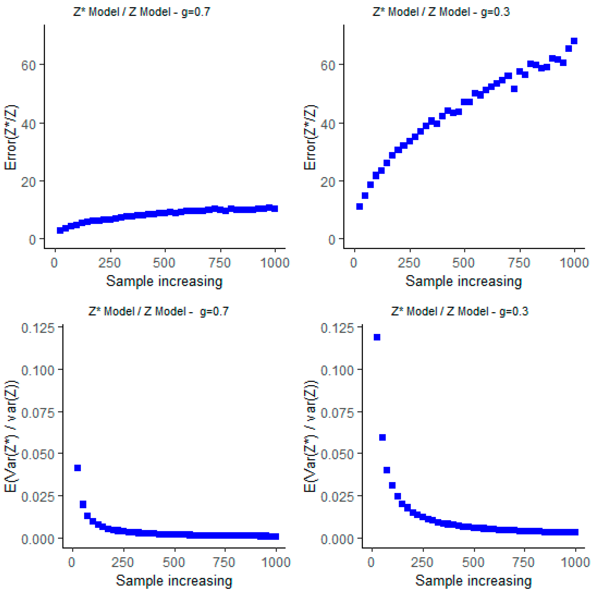
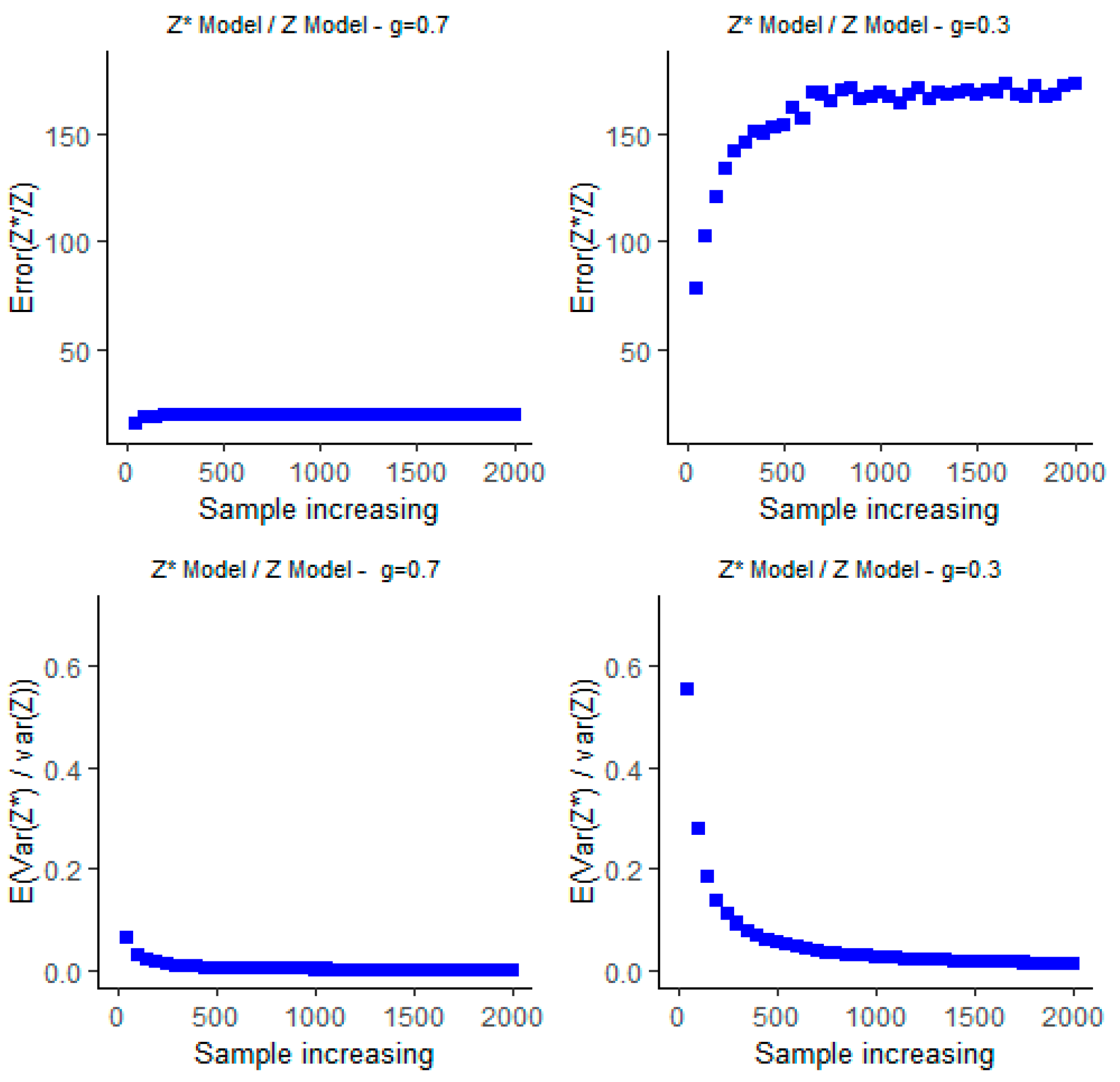
3.3. Graphical Simulation

Another way to analyze the behavior of Z* and Z with both databases is by visualizing the values of the following statistics: $Error\left(\frac{{RE}_{Z^{*}}}{{RE}_Z}\right)$ and $E\left(\frac{{\widehat{V}(Z}^{*})}{\widehat{V}\left(Z\right)}\right)$. For the first database, the sample size increases to n = 25, 50, …, 1000, and for the second database, the sample size increases to n = 50, 100, …, 2000. In the next figures, we can observe the accuracy and efficiency using both designs when we fixed $\alpha =0.5$, where g = 0.7 and g = 0.3.

In Figure 1, in terms of the accuracy of the estimator ${\widehat{\mu }}_Y$, it can be seen that it is better to use the Z model than the Z* model; as in the numerical results, it is more accurate to use the R₍₃₎ report (g = 0.3). Using the Z* model over the Z model with any report produces the minimum variance in the results. The graphs in Figure 2 agree with all the results already shown, where it is better to use the Z model for greater accuracy and the Z* model for the minimum variance.

4. Discussion

In this document, we propose a new randomized response technique, which allows us to obtain information on a variable of interest Y considered sensitive. In the study of the behavior of the proposed estimators, as already mentioned in this document, we treated the following as sensitive variables: the amount, in hectares, of destruction of poppy crops by the federal government of Mexico in the State of Guerrero and “At what age did you have your first sexual intercourse?”.

As a consequence of this study, for the first sensitive variable, it is preferable for researchers to use the proposed Z model to more accurately estimate the amount of poppy destruction. This is important in the national context since, due to the public policies of the current federal government [27] in implementing drug prevention programs or licit crop programs in order to reduce poppy crops, it is important to estimate what is closest to reality since, based on these estimates, the budgets for said programs are assigned. Otherwise, there would be an underestimation, causing an inadequate budget for the implementation of the programs, or an overestimation, which would cause other programs in other areas to have a lower budget. Neither sampling error is acceptable in a country such as Mexico.

In the analysis of the sensitive question “At what age did you have your first sexual intercourse?”, the same considerations can be made since the Z model provides the best estimate of the true value. On the other hand, if a researcher in the area of health [28], according to our sensitive variable, is also interested, in addition to knowing the estimated value of a sensitive characteristic, in knowing between which values the true value of this characteristic lies, that is, in building confidence intervals, it is better to use Z* due to its minimum variance, since it will provide smaller confidence intervals and, hypothetically, estimates with greater precision. This last statement is valid for unbiased estimators.

As a limitation of this work, the estimators in our proposal are as biased as in the work of Saleem et al. [21]. In our case, this is due to the use of ratio estimators, which, by their nature, are biased. In addition, the applicability of the ratio report R₍₃₎ is made more difficult in practical use compared to an addition, subtraction, or multiplication report. Finally, only a simple random sampling design was used.

For the aforementioned issues, it is recommended that, in future works, the estimators of the Z model under simple random sampling (SRS) be extended to stratified simple random sampling (SSRS). This variation is for the purpose of determining under which conditions it is better to use SRS or SSRS with the Z and Z* models, defining the gain in accuracy and optimal allocation, and so on. In addition, it would be desirable to propose other estimators that are not of the ratio type to make comparisons, in terms of accuracy and efficiency, with the estimators proposed in this document.

References

1. Jones, E.E.; Sigall, H. The bogus pipeline: A new paradigm for measuring affect and attitude. Psychol. Bull. 1971, 76, 349–364. [Google Scholar] [CrossRef] [Green Version]
2. Raghavarao, D.; Federer, W.T. Block Total Response as an Alternative to the Randomized Response Method in Surveys. J. R. Stat Soc. Ser. B 1979, 41, 40–45. [Google Scholar] [CrossRef] [Green Version]
3. Gupta, S.; Thornton, B. Circumventing Social Desirability Response Bias in Personal Interview Surveys. Am. J. Math. Manag. Sci. 2002, 22, 369–383. [Google Scholar] [CrossRef]
4. Warner, S.L. Randomized response: A survey technique for eliminating evasive answer bias. J. Am. Stat. Assoc. 1965, 60, 63–69. [Google Scholar] [CrossRef] [PubMed]
5. Bahadivand, S.; Doosti-Irani, A.; Karami, M. Prevalence of high-risk behaviors in reproductive age women in Alborz province in 2019 using unmatched count technique. BMC Women’s Health 2020, 20, 186. [Google Scholar] [CrossRef] [PubMed]
6. Greenberg, B.G.; Kuebler, R.R.J.; Abernathy, J.R.; Horvitz, D.G. Application of the Randomized Response Technique in Obtaining Quantitative Data. J. Am. Stat. Assoc. 1971, 66, 243–250. [Google Scholar] [CrossRef]
7. Eriksson, S.A. A new model for randomized response. Int. Stat. Rev. 1973, 41, 40–43. [Google Scholar] [CrossRef]
8. Huang, K.C. Estimation of sensitive characteristics using optional randomized technique. Qual. Quant. 2008, 42, 679–686. [Google Scholar] [CrossRef]
9. Bouza, C.N. Ranked set sampling and randomized response procedures for estimating the mean of a sensitive quantitative character. Metrika 2009, 70, 267–277. [Google Scholar] [CrossRef]
10. Arnab, R. Optional randomized response techniques for quantitative characteristics. Commun. Stat. Theory Methods 2018, 48, 4154–4170. [Google Scholar] [CrossRef]
11. Singh, H.P.; Gorey, S. On Two Stage Optional Randomized Response Model. Elixir Stat. 2018, 123C, 51963–51987. [Google Scholar]
12. Hussain, Z.; Shahid, M.I. Improved Randomized Response in Optional Scrambling Models. J. Stat. Theory Pract. 2019, 18, 351–360. [Google Scholar] [CrossRef] [Green Version]
13. Narjis, G.; Shabbir, J.; Onyango, R. Partial Randomized Response Model for Simultaneous Estimation of Means of Two Sensitive Variables. Math. Probl. Eng. 2022, 2022, 1–13. [Google Scholar] [CrossRef]
14. Bouza-Herrera, C.N.; Juárez-Moreno, P.O.; Santiago-Moreno, A.; Sautto-Vallejo, J.M. A Two-Stage Scrambling Procedure: Simple and Stratified Random Sampling. An Evaluation of COVID 19’s data in Mexico. Investig. Oper. 2022, 43, 421–430. [Google Scholar]
15. Hussain, Z.; Shakeel, S.; Cheema, S.A. Estimation of stigmatized population total: A new additive quantitative randomized response model. Commun. Stat. Theory Methods 2022, 51, 8741–8753. [Google Scholar] [CrossRef]
16. Azeem, M.; Ali, S. A neutral comparative analysis of additive, multiplicative, and mixed quantitative randomized response models. PLoS ONE 2023, 18, 4. [Google Scholar] [CrossRef]
17. Murtaza, M.; Singh, S.; Hussain, Z. Use of correlated scrambling variables in quantitative randomized response technique. Biom. J. 2020, 63, 134–147. [Google Scholar] [CrossRef]
18. Chong, A.; Chu, A.; So, M.; Chung, R. Asking Sensitive Questions Using the Randomized Response Approach in Public Health Research: An Empirical Study on the Factors of Illegal Waste Disposal. Int. J. Environ. Res. Public Health 2019, 16, 970. [Google Scholar] [CrossRef] [Green Version]
19. Perri, P.F.; Cobo-Rodríguez, B.; Rueda-García, M. A mixed-mode sensitive research on cannabis use and sexual addiction: Improving self-reporting by means of indirect questioning techniques. Qual. Quant. 2018, 52, 1593–1611. [Google Scholar] [CrossRef]
20. Kirtadze, I.; Otiashvili, D.; Tabatadze, M.; Vardanashvili, I.; Sturua, L.; Zabransky, T.; Anthony, J.C. Republic of Georgia estimates for prevalence of drug use: Randomized response technique suggest under-estimation. Drug Alcohol. Depend. 2018, 187, 300–304. [Google Scholar] [CrossRef]
21. Saleem, I.; Sanaullah, A.; Koyuncu, N. Estimation of Mean of a Sensitive Quantitative Variable in Complex Survey: Improved Estimator and Scrambled Randomized Response Model. J. Sci. 2019, 32, 1021–1043. [Google Scholar]
22. México Unido Contra La Delincuencia. Datos Abiertos Sobre Acciones Antidrogas. Available online: https://www.mucd.org.mx (accessed on 19 January 2023).
23. De Salud, S. Encuesta Nacional de Salud y Nutrición. Available online: https://www.ensanut.insp.mx (accessed on 19 January 2023).
24. Epstein, M.; Bailey, J.; Manhart, L.; Hill, K.; Hawkins, D.; Haggerty, K.; Catalano, R. Understanding the Link Between Early Sexual Initiation and Sexually Transmitted Infection: Test and Replication in Two Longitudinal Studies. J. Adolesc. Health. 2014, 54, 435–441. [Google Scholar] [CrossRef] [PubMed] [Green Version]
25. Brener, N.D.; Eaton, D.K.; Kann, L. The Association of Survey Setting and Mode with Self-Reported Health Risk Behaviors Among High School Students. Public. Opin. Q. 2014, 70, 354–374. [Google Scholar] [CrossRef] [Green Version]
26. Singh, S. Advanced Sampling Theory with Application, 1st ed.; Kluwer Academic Publishers: Dordrecht, The Netherlands, 2003. [Google Scholar]
27. México, Monitoreo de Plantíos de Amapola 2019–2020. Available online: https://www.unodc.org (accessed on 23 January 2023).
28. Candia, R.; Caiozzi, G. Intervalos de confianza. Rev. Méd. Chile 2005, 133, 1111–1115. [Google Scholar] [CrossRef] [PubMed] [Green Version]
Figure 1. Accuracy and efficiency under Z* and Z in database of illicit crops.
Mathematics 11 02572 g001
Figure 2. Accuracy and efficiency under Z* and Z in database of first sexual intercourse.
Mathematics 11 02572 g002