Global–Local Non Intrusive Analysis with 1D to 3D Coupling: Application to Crack Propagation and Extension to Commercial Software

Abstract

Computational simulation is a highly reliable tool used to solve structural analysis problems. In recent times, several techniques have been developed in the field of computational mechanics in order to analyze non-linearities in less time, helping decision-making when structures suffer damage. The global–local analysis is a technique to increase the efficiency of computational simulations by using a global model to obtain boundary conditions in a coupling zone imposed on a local model. Coupling can be performed through the primal–dual method, which is used for crack propagation using 2D and 3D models with fine meshes, thus saving computational time. However, it has not been implemented at a commercial level to analyze large structures such as multi-story buildings with focused non-linearities. In this work, a global–local analysis with non-intrusive methodology and simplified models was implemented in a cracked framed structure, using a 1D (global) and 3D (local) coupling considering crack propagation with primal–dual interface conditions. Different lengths of the local model were analyzed, studying their influence on the convergence of the problem, and compared with a 3D monolithic model to check the reliability of the results. The results show that the proposed methodology solves the problem with an error less than 10%. Furthermore, it was determined that the dimensions of the local model affect the convergence of the problem. This work also provides an implementation of the method for large structures containing focused non-linearities and using commercial software, reducing computational time for the cracked structural analysis.

1. Introduction

The structures are designed to withstand different internal forces such as traction, compression, bending, cutting, torsion and combined forces. In addition, fatigue damage and seismic provisions must be considered in the design of structural steel buildings [1,2]. The performance of the structure is diminished under the effect of factors such as corrosion, maintenance and the nature of cyclic loads [3], producing increased stress, cracking and subsequent fracture of the material [4]. For these cases, numerical calculation methodologies based on finite elements have been developed to predict the behavior of structures with the presence of cracks, such as the extended finite element method (X-FEM) [5,6], which consists of discretizing a continuum using a mesh, and solving roughly at the nodes and then interpolate to the rest of the element. However, if a singularity occurs, it incorporates enriched shape functions to simulate this phenomenon, allowing the mesh to generate discontinuities and adapt as the problem changes, thus avoiding the remeshing of the problem [7].

However, for large structures subject to static and dynamic loads, these are calculated using beam elements (1D elements with 6 degrees of freedom per node) [8,9]. Even so, these types of elements do not account for crack propagation in their formulations, which means that to study this behavior, other types of complex modeling must be used at a higher computational cost. Therefore, to deal with large structures, multiscale methods have been developed, some of which are based on domain decomposition [10,11,12,13,14,15] that allow linking models to perform structural analysis of complex structures. Although these techniques have shown good performance in academic applications, they are rarely applied to practical industrial cases. Thus, in order for them to be useful in the industry, it is necessary to validate the simulations with these methods and ensure their computational efficiency and escalability [16]. The implementation of multiscale methods requires a high cost in time and computational resources, in addition to needing methods to link the different scales [16].

Based on domain decomposition methods, the global–local analysis [17] was developed, in order to improve the convergence of complex simulations. This technique uses an approximate global model with a coarse mesh and typically linear to obtain appropriate boundary conditions, which are imposed on the local model in the coupling zone, solving the latter independently.

In [18], is proposed a non-intrusive global–local coupling algorithm based on domain decomposition method, intended for large-scale non-linear analysis without the need to modify the solver base code global model [19]. In [20], the strategy is interpreted as an alternative decomposition method of optimized and non-overlapping Schwarz domains, improving the results. The non-intrusive global–local coupling is applied for complex non-linear behavior (plastic hardening, crack propagation, among others) in [21].

The non-intrusive method uses linear and non-linear solvers as a black box, which are optimized and already incorporated into commercial software to introduce these solutions in the form of displacements and/or forces in a linear model of the entire structure without modifying it (non-intrusive) [15].

An example of non-intrusivity is to use the tools provided by the free software Code_Aster [22] that uses XFEM to solve crack propagation problems and through a Python interface, linking it with its linear solver (FEM) or with other commercial software, such as SAP2000 which is used in this work. Other works where SAP 2000 software is used for different types of analysis can be reviewed in [23,24,25,26], among others. However, other commercial software has been used to analyze crack propagation and complex simulations, such as ANSYS [27,28,29] and Abaqus [30,31,32,33,34]. This methodology has been implemented in a two-dimensional domain with crack growth and mesh refinement in [19,35,36], as well as in analysis with plastic behavior with mesh refinement in [19,37], where the implementation for a three-dimensional domain was also studied. In addition, asynchronous global–local methods have been studied, allowing an improvement in execution times for complex structures [38,39].

In [21], Robin parameters or mixed coupling [15,35,40] was studied to improve the execution times. In these studies, a Robin parameter optimization was performed in 2D and 3D problems with crack growth and plastic hardening to improve the convergence of mixed global–local non-intrusive analysis.

In order to improve the performances of the mixed strategy, industrial problems have been analyzed by means of a two-scale approximation of Schur’s complement as a Robin condition in the local model [41,42] being applied in models of an aircraft turbine blade, or other applications such as mechanical and hydraulic fracture modeling [35,43].

This work focuses on implementing a global–local non-intrusive analysis methodology using primal–dual coupling in a global model with 1D elements and a complex local model using 3D formulation, which presents crack growth. Specifically, the XFEM method is used to analyze the crack propagation without remeshing the model [5,6] implemented in different steel moment resisting frames, with a 250 Mpa yield strength.

The non-intrusive strategy is implemented in a frame structure that presents a localized crack. First, the software Code_Aster and the Python interface were used. Then, it is solved by linking Code_Aster and the commercial software SAP2000, obtaining a methodology that allows us to reduce the degrees of freedom analyzed, impacting the computational resolution time. The proposed methodology is validated by simulating a 3D monolithic model solved with the Code_Aster software.

The work is organized as follows. The methodology section presents the study case, software used and the formulation of the primal–dual coupling methodology for 1D and 3D models. In the results and analysis section, the validation of the methodology is shown, together with the convergence comparison of the study cases. Subsequently, the application of the methodology using the commercial software SAP 2000, the validation of the method using this software and the application in a large structure are analyzed. Finally, the discussion section summarizes the work conducted and also presents future studies regarding this topic.

2. Methodology

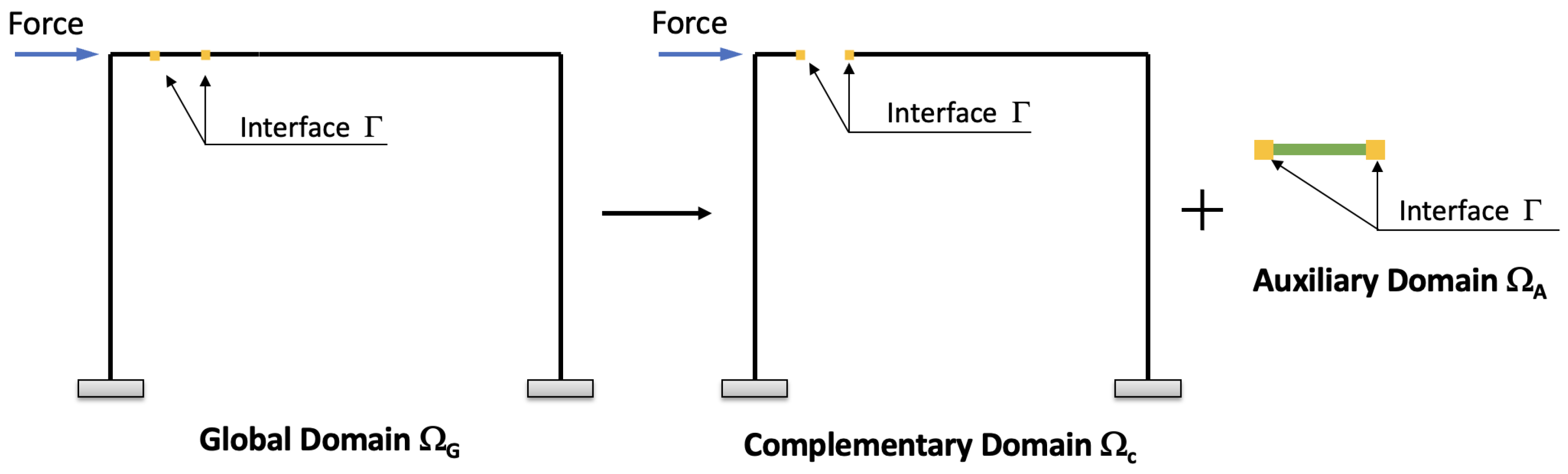
2.1. Primal–Dual Global–Local Analysis

Performing a global–local analysis on a structure with non-linearities (Figure 1) consists of separating the linear elastic global domain ${\mathsf{\Omega }}_R$ of the structure (Figure 2) into two linear non-overlapping domains, the complementary domain ${\mathsf{\Omega }}_C$ and auxiliary domain ${\mathsf{\Omega }}_A$. The auxiliary domain is duplicated on a 3D non-linear (with crack propagation) local domain ${\mathsf{\Omega }}_L$ (Figure 3). The interfaces between subdomains are connected with linear $\mathsf{\Gamma }$ interfaces. The detailed formulation and mathematical background (functional spaces, Lagrangian definition, Lagrange multipliers among others) can be found in [21].

When implementing this methodology, the mechanical problem of each domain in which it was discretized (global, auxiliary and local models) must be solved for each iteration. Therefore, the problem to solve is the following:

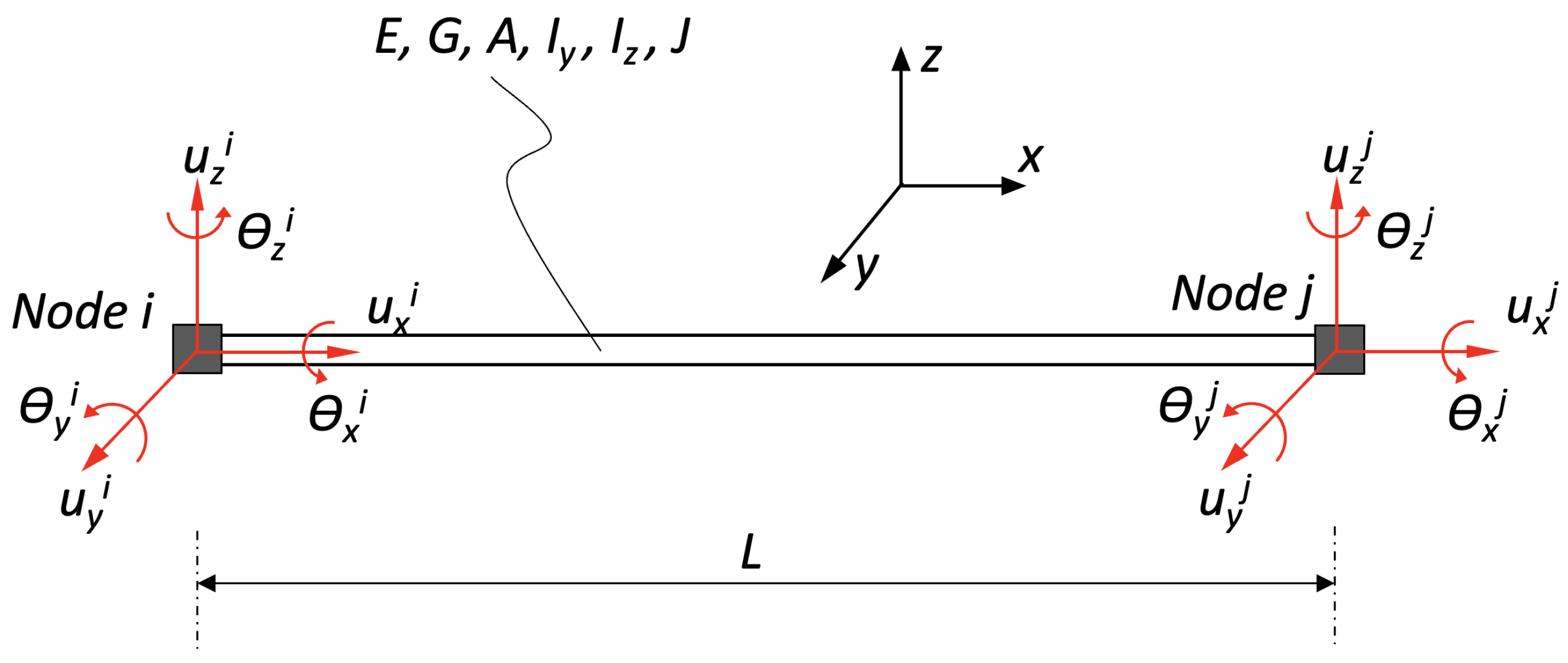
• First, the global problem is solved by obtaining the displacements $u_G^{n+1}$:

  $$K_G{u}_G^{n+1}=f_d^G+C_G^T{P}^n$$

  (1)

  where $K_G$ is the stiffness matrix of the global model, $f_d^G$ is the external load vector in the domain ${\mathsf{\Omega }}_G$, $C_G$ is a coupling operator of the global problem that relates the degrees of freedom of the interface with respect to the degrees of freedom of the complete domain, and $P^n$ is the compensation force (vector) of the previous iteration. For the first iteration, $P^n$ is a vector of zeros for a 3D frame global model with an interface of two nodes.
• Second, the auxiliary problem is solved by imposing the displacements $u_A^{n+1}{|}_{\mathsf{\Gamma }}$ and solve for the reaction forces ${\lambda }_A^{n+1}$ in the interface zone:

  $$K_A{u}_A^{n+1}{|}_{\mathsf{\Gamma }}-C_A^T{\lambda }_A^{n+1}=f_d^A$$

  (2)

  where $K_A$ is the stiffness matrix of the auxiliary model, $f_d^A$ is the external load vector, and ${\lambda }_A^{n+1}$ is the reaction force at the interface for the domain ${\mathsf{\Omega }}_A$.
  The ${\lambda }_A^{n+1}$ can be obtained directly in some software, allowing the obtainment of the reaction forces from embedded structures within a global problem.
  The displacements $u_A^{n+1}{|}_{\mathsf{\Gamma }}$ can be extracted from the solution of the global problem using the following relation:

  $$u_A^{n+1}{|}_{\mathsf{\Gamma }}=C_A{u}_A^{n+1}=C_G{u}_G^{n+1}$$

  (3)

  where $C_A$ is a coupling operator that relates the degrees of freedom of the interface with respect to the Auxiliary domain ${\mathsf{\Omega }}_A$ and $C_G$ was previously defined.
• Third, the local problem is solved by imposing the displacements $u_L^{n+1}{|}_{\mathsf{\Gamma }}$ on the interface of the local model

  $$u_L^{n+1}{|}_{\mathsf{\Gamma }}=C_L{u}_L^{n+1}={\mathbf{Pr}}_{\mathbf{GL}}\left\{C_G{u}_G^{n+1}\right\}$$

  (4)

  where $C_L$ is an operator that relates the degrees of freedom of the interface with respect to the degrees of freedom of the local domain ${\mathsf{\Omega }}_L$, $u_L^{n+1}{|}_{\mathsf{\Gamma }}$ are the displacement on the interface of the local model and ${\mathbf{Pr}}_{\mathbf{GL}}$ is a projection operator, from the global 1D model to the local 3D domain. The formulation of this projector is presented in Section 2.3.
  Hence, the reaction forces ${\lambda }_L^{n+1}$ of the local model in the interface, solved by means of a nonlinear solver such as Arc Length Method [44] or Newthon–Raphson Method, is obtained from the following equation:

  $$K_L{u}_L^{n+1}{|}_{\mathsf{\Gamma }}-C_L^T{\lambda }_L^{n+1}=f_d^L$$

  (5)

  where $K_L$ is the stiffness matrix of the local model, $f_d^L$ is the external load vector in the domain ${\mathsf{\Omega }}_L$ and ${\lambda }_L^{n+1}$ is the reaction force at the interface.
• Fourth, the correction forces that will be applied to the global model $P^n$ are calculated:

  $$P^{n+1}={\lambda }_A^{n+1}+{\mathbf{Pr}}_{\mathbf{LG}}\left\{{\lambda }_L^{n+1}\right\}$$

  (6)

  where the projector operator ${\mathbf{Pr}}_{\mathbf{LG}}$, from the local to the global domain, is also presented in Section 2.3 and is used with a Code_Aster built-in function.
• Fifth, the residual force $r^{n+1}$ is calculated and the error $\eta$ of the solution obtained in the iteration is estimated:

  $$r^{n+1}=P^{n+1}-P^n$$

  (7)

  $$\eta =\Vert r^{n+1}{\Vert }_2/{\Vert r^0\Vert }_2$$

  (8)
• Finally, a relaxation scheme is considered, obtaining the following correction force:

  $$P^{n+1}=\mu P^{n+1}+(1-\mu )P^n$$

  (9)
  This relaxation allows for better convergence, for example, when Aitken ${\delta }^2$ relaxation method is used [19].

The compensation forces $P_n$ assigned in the interface $\mathsf{\Gamma }$ of the global model (Figure 2) are applied to represent the local non-linear effects on the global model. These forces have 6 components for each node analyzed, as shown in Equation (10), since the force correction is performed in the global model.

$$P_n={\left[FxFyFzMxMyMz\right]}^T$$

(10)

It is important to mention that the coupling operators $C_A$, $C_G$, and $C_L$ are sparse matrices, which relate the total degrees of freedom of each model to its interface.

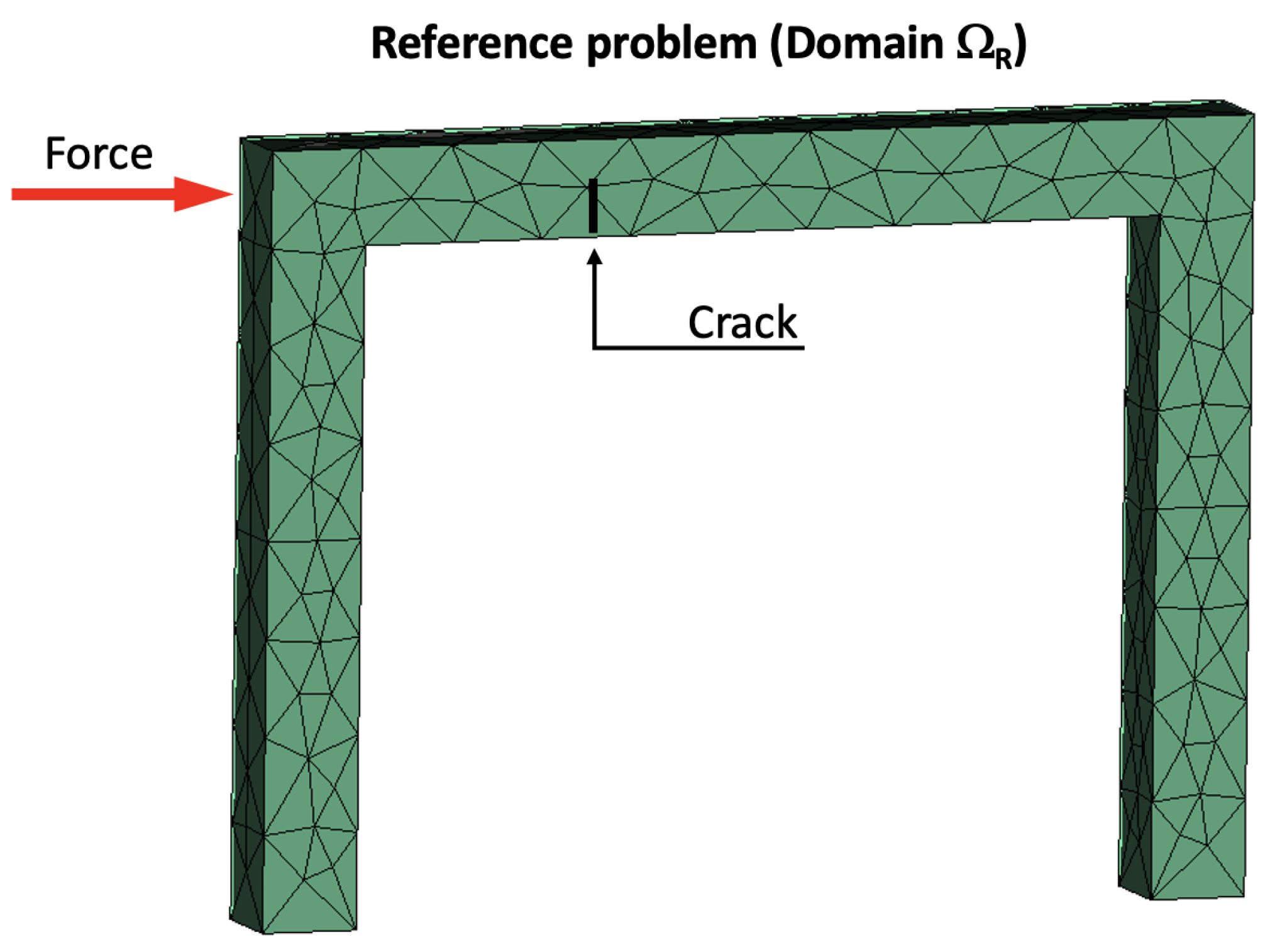
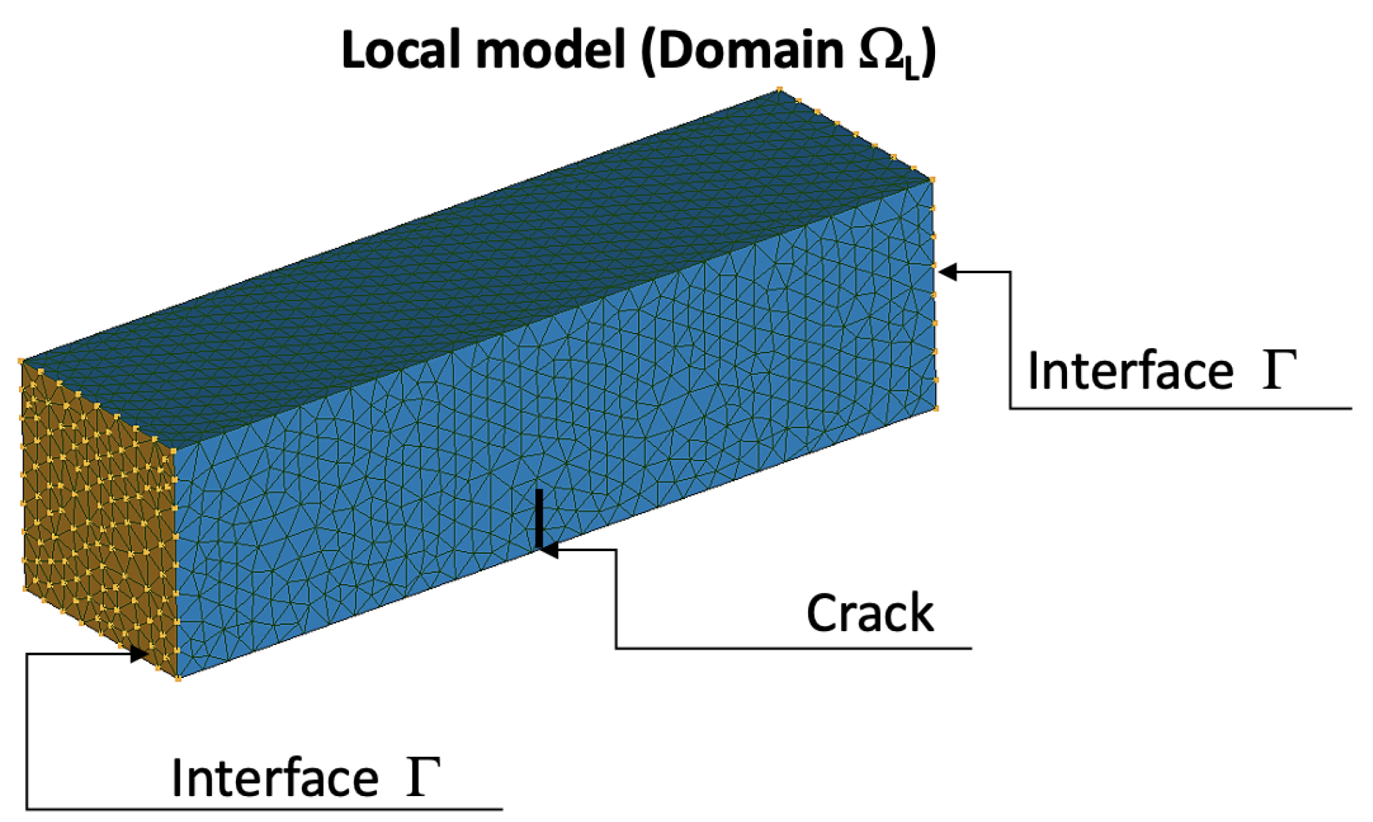
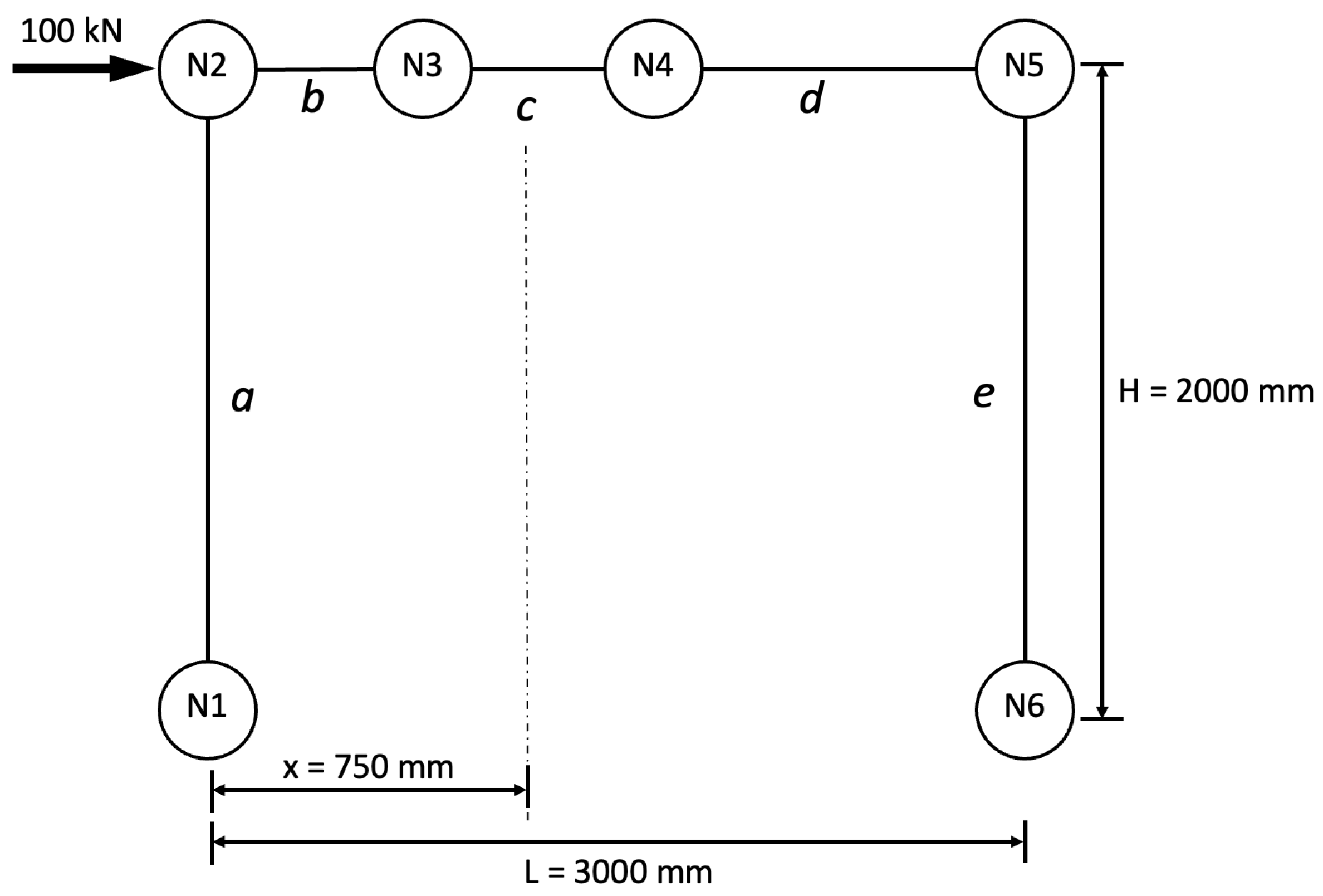
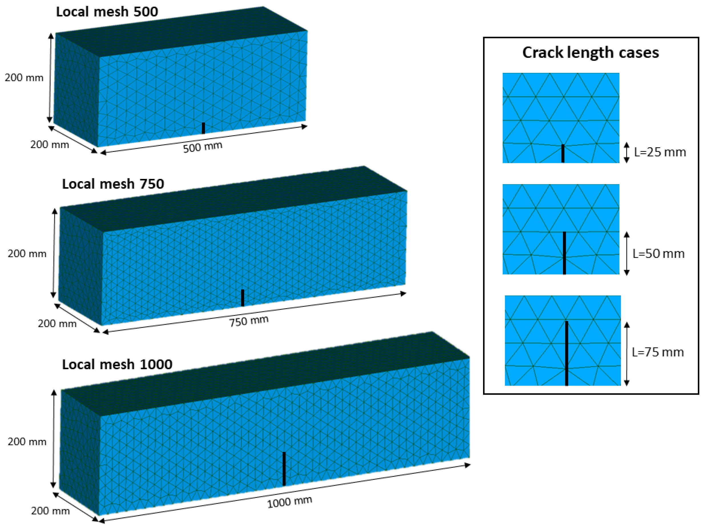
2.2. Case Study

The steel frame used for the analysis is made up of a 3-meter-long beam and two two-meter-long columns, whose joints between them are considered rigid, as is the support of the columns. The section of the elements is a square section of two hundred millimeters on each side. The material used is a steel with a yield limit of 250 MPa, a modulus of elasticity equal to 200,000 MPa and a Poisson’s ratio of 0.3.

The 1D model of the frame is discretized into six nodes and five elements (elements “a” to “e”), as can be seen in Figure 4, where the length of the element “c” is used to generate the local model and will be centered in the position x = 750 mm (crack location). Nodes 3 and 4 are the interface between domains to perform the non-intrusive coupling and at node 2 a horizontal force of 100 kN is applied. The global model of the considered frame has six degrees of freedom ($u_x,u_y,u_z,{\theta }_x,{\theta }_y,{\theta }_z$), while the local model, being modeled by 3D elements, only considers three degrees of freedom ($u_x,u_y,u_z$). Finally, nodes 1 and 6 correspond to fixed supports with restricted rotations.

The Code_Aster software was used for linear and non-linear analysis. Code_Aster has modules implemented to study crack growth using the XFEM methodology [5,6], without remeshing the local problem and allowing to analyze several propagation steps predefined by the user.

The global model is defined according to the Euler-Bernoulli beam theory and with linear behavior. The effects of the shear deformation energy are neglected in the stiffness matrix of the 1D frame elements, as presented in Equation (11), for the corresponding element shown in Figure 5.

$$K_{frame1D}=\left[\begin{array}{cc}{K}_{11}& K_{12}\\ K_{21}& K_{22}\end{array}\right]$$

(11)

where matrices $K_{11}$, $K_{12}$, $K_{21}$ and $K_{22}$ are defined in Equations (12), (13), (14) and (15), respectively:

$$K_{11}=\left[\begin{array}{cccccc}EA/L& 0& 0& 0& 0& 0\\ 0& 12E{I}_z/L^3& 0& 0& 0& 6E{I}_z/L^2\\ 0& 0& 12E{I}_y/L^3& 0& -6E{I}_y/L^2& 0\\ 0& 0& 0& GJ/L& 0& 0\\ 0& 0& -6E{I}_y/L^2& 0& 4E{I}_y/L& 0\\ 0& 6E{I}_z/L^2& 0& 0& 0& 4E{I}_z/L\end{array}\right]$$

(12)

$$K_{12}=\left[\begin{array}{cccccc}-EA/L& 0& 0& 0& 0& 0\\ 0& -12E{I}_z/L^3& 0& 0& 0& 6E{I}_z/L^2\\ 0& 0& -12E{I}_y/L^3& 0& -6E{I}_y/L^2& 0\\ 0& 0& 0& -GJ/L& 0& 0\\ 0& 0& 6E{I}_y/L^2& 0& 2E{I}_y/L& 0\\ 0& -6E{I}_z/L^2& 0& 0& 0& 2E{I}_z/L\end{array}\right]$$

(13)

$$K_{21}=K_{12}$$

(14)

$$K_{22}=\left[\begin{array}{cccccc}EA/L& 0& 0& 0& 0& 0\\ 0& 12E{I}_z/L^3& 0& 0& 0& -6E{I}_z/L^2\\ 0& 0& 12E{I}_y/L^3& 0& 6E{I}_y/L^2& 0\\ 0& 0& 0& GJ/L& 0& 0\\ 0& 0& 6E{I}_y/L^2& 0& 4E{I}_y/L& 0\\ 0& -6E{I}_z/L^2& 0& 0& 0& 4E{I}_z/L\end{array}\right]$$

(15)

where $I_y$ and $I_z$ corresponds to the second moment of area in the y and z axis, respectively, A is the section area, L is the length of the element and J is Saint Venant’s or torsional constant of the section. The material constants are E and G corresponding to the Young modulus and shear modulus of the material, respectively.

For the 3D tetrahedral element, the stiffness matrix is calculated using the constitutive matrix D presented in Equation (16) and the degrees of freedom are presented in Figure 6.

$$D=\frac{E(1-\nu )}{(1+\nu )(1-2\nu )}\left[\begin{array}{cccccc}1& \frac{\nu }{1-\nu }& \frac{\nu }{1-\nu }& 0& 0& 0\\ & 1& \frac{\nu }{1-\nu }& 0& 0& 0\\ & & 1& 0& 0& 0\\ & & & \frac{1-2\nu }{2(1-\nu )}& 0& 0\\ Symmetrical& & & & \frac{1-2\nu }{2(1-\nu )}& 0\\ & & & & & \frac{1-2\nu }{2(1-\nu )}\end{array}\right]$$

(16)

where $\nu$ and E correspond to the Poisson modulus and the Young Modulus of the material. Therefore, the stiffness matrix of a single element $K^e$ is presented in Equation (17).

$$K^e=\left[\begin{array}{cccc}{K}_{11}^e& K_{12}^e& K_{13}^e& K_{14}^e\\ & K_{22}^e& K_{23}^e& K_{24}^e\\ & & K_{33}^e& K_{34}^e\\ Symmetrical& & & K_{44}^e\end{array}\right]$$

(17)

where each term of the stiffness matrix can be calculated using the expression presented in Equation (18).

$$K_{ij}^e=\frac{1}{36V^{\left(e\right)}}\left[\begin{array}{ccc}(d_{11}{b}_i{b}_j+d_{44}{c}_i{c}_j+d_{55}{d}_i{d}_j)& (d_{12}{b}_i{c}_j+d_{44}{b}_i{c}_j)& (d_{13}{b}_i{d}_j+d_{55}{b}_i{b}_j)\\ (d_{21}{c}_i{b}_j+d_{44}{b}_i{c}_j)& (d_{22}{c}_i{c}_j+d_{44}{b}_i{b}_j+d_{66}{d}_i{d}_j)& (d_{23}{c}_i{d}_j+d_{66}{d}_i{c}_j)\\ (d_{31}{d}_i{b}_j+d_{55}{b}_i{d}_j)& (d_{32}{d}_i{c}_j+d_{66}{c}_i{d}_j)& (d_{33}{d}_i{d}_j+d_{55}{b}_i{b}_j+d_{66}{c}_i{c}_j)\end{array}\right]$$

(18)

where $d_{i,j}$ corresponds to the terms of the constitutive matrix D of Equation (16) and the terms $c_i$ are the terms of the matrix $B_i$ that presents the derivatives of the linear shape functions $N_i$ for each node i, as presented in Equation (19).

$$B_i=\left[\begin{array}{ccc}\frac{\partial N_i}{\partial x}& 0& 0\\ 0& \frac{\partial N_i}{\partial y}& 0\\ & & \frac{\partial N_i}{\partial z}\\ \frac{\partial N_i}{\partial y}& \frac{\partial N_i}{\partial x}& 0\\ \frac{\partial N_i}{\partial z}& 0& \frac{\partial N_i}{\partial x}\\ 0& \frac{\partial N_i}{\partial z}& \frac{\partial N_i}{\partial y}\end{array}\right]=\frac{1}{6V^{\left(e\right)}}\left[\begin{array}{ccc}{b}_i& 0& 0\\ 0& c_i& 0\\ 0& 0& d_i\\ c_i& b_i& 0\\ d_i& 0& b_i\\ 0& d_i& c_i\end{array}\right]$$

(19)

The shape functions $N_i$ are linear functions that interpolates the displacement field from the nodes into the element $V^e$, as presented in the classical Finite Element Methods [45].

In the case of the non-linear problem, 3D tetrahedral finite elements with linear shape functions are considered and XFEM is used for the calculation of crack growth (with 3 propagation steps). To analyze the convergence of the problem, three crack lengths (25 mm, 50 mm, and 75 mm) are considered, analyzing each one with three different local mesh lengths, as presented in Figure 7. Each mesh length will be named as follows:

• Local Mesh 1 (L.M. 1): Length 500 mm
• Local Mesh 2 (L.M. 2): Length 750 mm
• Local Mesh 3 (L.M. 3): Length 1000 mm

For the crack propagation of the local model, the crack is initialized and the location is defined (as described before in Figure 7). Code_Aster also required the following inputs for the crack propagation procedure:

• The direction of propagation is taken into account, with a tangent vector (0,0,1) and normal vector (1,0,0) with the function $DEFI\_FISS\_XFEM$ of Code_Aster.
• The propagation is calculated internally, calculating the energy release rate using the intensity factors with the function $CALC\_K\_G$ of Code_Aster for a predefined number of propagation steps (function $PROPA\_FISS$).

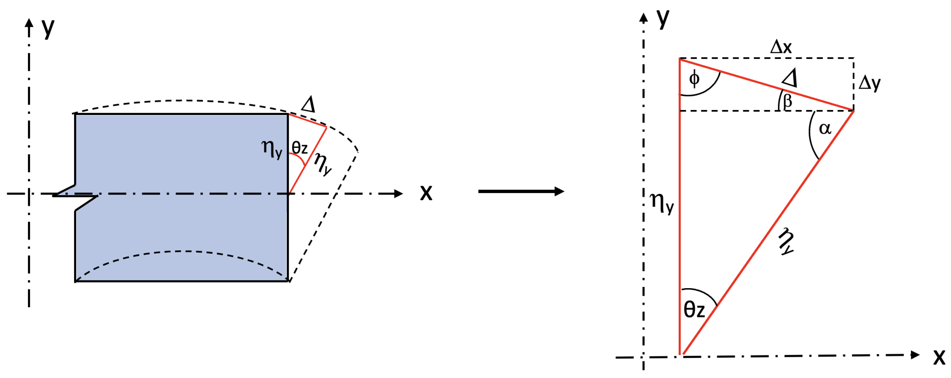
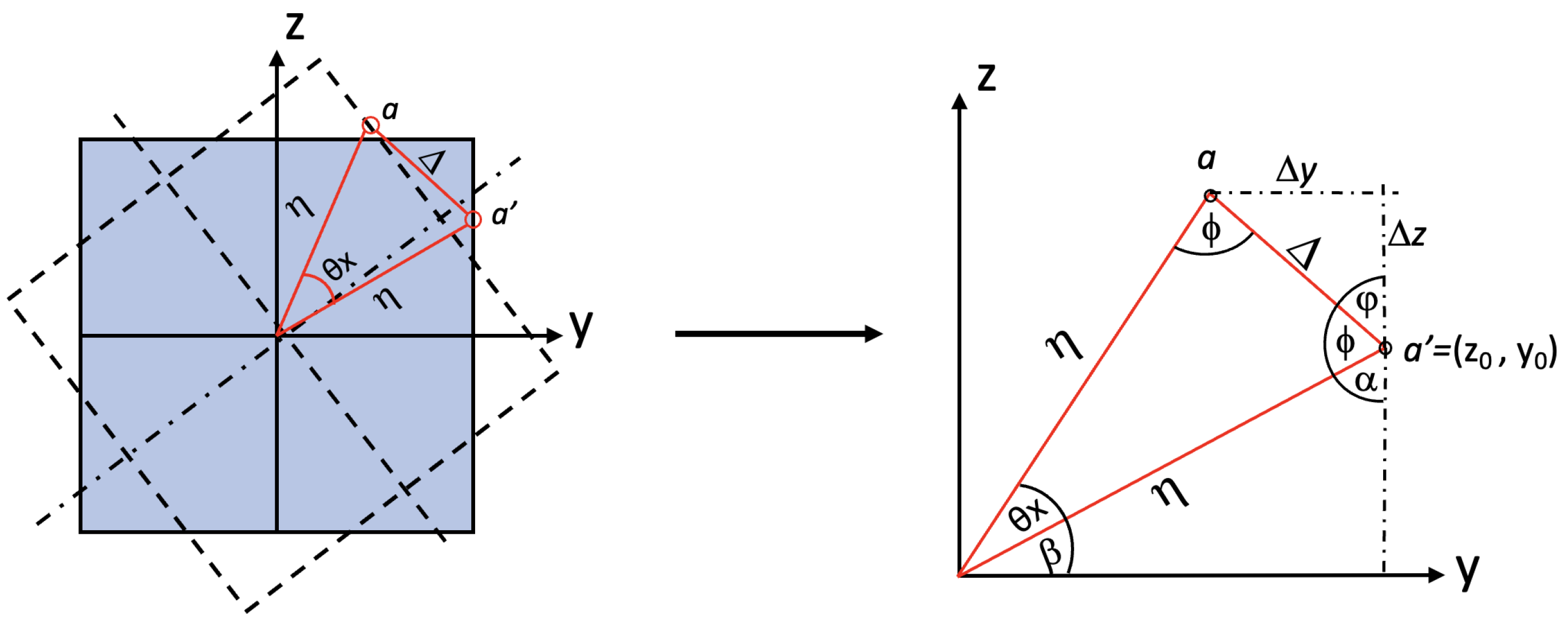
2.3. Projection of Displacements from the Global 1D Model to the Local 3D Model

When using 1D and 3D models for the implementation of a primal–dual analysis, there is no coincidence in the nodes of the different meshes. Hence, the projection of the results of one model to another must be carried out. Solving a 1D model subject to bending, torsion, and displacement in all 3 axes results in displacements and rotations that must be accounted for when projecting displacements.

The projection of the displacements and rotations was implemented using a Python function that takes as input parameters the displacements obtained in the global 1D model analysis ($u_x,u_y,u_z,{\theta }_x,{\theta }_y,{\theta }_z$) and the data of the local mesh. As output returns the displacements of all nodes ($u_x$, $u_y$ and $u_z$) of the local model. This procedure is used to built the operator ${\mathbf{Pr}}_{\mathbf{GL}}\{☐\}$, as presented in Equation (4).

Thus, the procedure for projecting nodal displacements of the 1D global model (degrees of freedom $u_x$, $u_y$, $u_z$ and rotations ${\theta }_x$, ${\theta }_y$ and ${\theta }_z$) are presented below. Specifically, for the rotation in the y direction ${\theta }_y$ the steps are:

1.

To calculate the displacement generated from the rotation resulting from bending ${\theta }_y$, kinematic compatibility is considered, using a non-deformable finite element (solid face with no warping) and rotating with respect to the centroid. The face of the 3D element analyzed has a maximum distance ${\eta }_z$ from the centroid and when rotated it is maintained, producing a displacement $\Delta$, as shown in Figure 8.

2.

Then, the displacement components are determined geometrically, i.e., the angles of the figure and considering them as a function of ${\theta }_y$, thus solving the value of $\Delta$ based on known parameters (${\eta }_z$ and ${\theta }_y$). The final expressions are shown in Equations (20) and (21).

$$\begin{array}{c}\hfill \frac{sin{\theta }_y}{\Delta }=\frac{sin(90-\frac{{\theta }_y}{2})}{{\eta }_z}\end{array}$$

(20)

$$\begin{array}{c}\hfill \Delta =\frac{{\eta }_{z}sin{\theta }_y}{sin(90-\frac{{\theta }_y}{2})}\end{array}$$

(21)

3.

Finally, the values of ${\Delta }_x$ and ${\Delta }_z$ are found, which would be the effects that must be considered due the bending rotations, leading to the following expressions:

$$\begin{array}{c}\hfill {\Delta }_x=\Delta cos\left(\frac{{\theta }_y}{2}\right)\end{array}$$

(22)

$$\begin{array}{c}\hfill {\Delta }_z=\Delta sin\left(\frac{{\theta }_y}{2}\right)\end{array}$$

(23)

Thus, the total displacement that is imposed on each node for the rotation ${\theta }_y$ is $u_x+{\Delta }_x$ and $u_z+{\Delta }_z$.

For the ${\theta }_z$ rotation due to bending, as shown in Figure 9, the equations are obtained using the same methodology presented above, obtaining the Equations (24)–(27).

$$\begin{array}{c}\hfill \frac{sin{\theta }_z}{\Delta }=\frac{sin(90-\frac{{\theta }_z}{2})}{{\eta }_y}\end{array}$$

(24)

$$\begin{array}{c}\hfill \Delta =\frac{{\eta }_{y}sin{\theta }_z}{sin(90-\frac{{\theta }_z}{2})}\end{array}$$

(25)

$$\begin{array}{c}\hfill {\Delta }_x=\Delta cos\left(\frac{{\theta }_z}{2}\right)\end{array}$$

(26)

$$\begin{array}{c}\hfill {\Delta }_y=\Delta sin\left(\frac{{\theta }_z}{2}\right)\end{array}$$

(27)

where ${\theta }_z$ is the bending rotation along the Z axis and ${\eta }_y$ is the distance from the centroid in the Y direction.

In the event that the structure is subjected to torsional moment, this effect must be considered in the local model imposed displacements.

Figure 10 will be used to determine the displacements imposed due to torsion (rotation in the “x” axis). Lets consider that the point a’ represents a node of the element that will be rotated to a position a given an angle ${\theta }_x$, generating a displacement $\Delta$ whose components will represent the mentioned effects.

The procedure to analyze the effects of the torsional rotation ${\theta }_x$ is presented below:

1.

The first thing will be to determine the value of the angles based on ${\theta }_x$ and $\beta$, where the latter represents the initial angle of the node with respect to the origin. Then, the value of $\eta$ must be calculated, obtaining the expressions shown in Equations (28) and (29) are obtained.

$$\begin{array}{c}\hfill \eta =\sqrt{y_0^2+z_0^2}\end{array}$$

(28)

$$\begin{array}{c}\hfill \Delta =\frac{\left(\sqrt{y_0^2+z_0^2}\right)sin{\theta }_x}{sin(90-\frac{{\theta }_x}{2})}\end{array}$$

(29)

2.

Then, the values of ${\Delta }_y$ and ${\Delta }_z$ are found, which would be the effects on the displacement due to torsional moment, leading to:

$$\begin{array}{c}\hfill {\Delta }_z=\frac{\left(\sqrt{y_0^2+z_0^2}\right)sin{\theta }_x}{sin(90-\frac{{\theta }_x}{2})}cos\left(\frac{{\theta }_x}{2}\right)\end{array}$$

(30)

$$\begin{array}{c}\hfill {\Delta }_y=\frac{\left(\sqrt{y_0^2+z_0^2}\right)sin{\theta }_x}{sin(90-\frac{{\theta }_x}{2})}sin\left(\frac{{\theta }_x}{2}\right)\end{array}$$

(31)

In addition to the displacements from 1D to 3D, the nodal forces of the local model must be transferred to resultant forces and moments to calculate the compensation forces that are imposed on the global 1D model. To that end, the sum of the nodal forces in each direction is performed and the resulting moment with respect to the centroid is calculated, through the function of Code_Aster $POST\_RELEVE\_T$, integrating the stresses and returning 3 forces and 3 moments (one for each axis, respectively) and used in Equation (6) of the iterative analysis procedure in the operator ${\mathbf{Pr}}_{\mathbf{LG}}\{☐\}$.

3. Implementation of the Methodology in Code_Aster

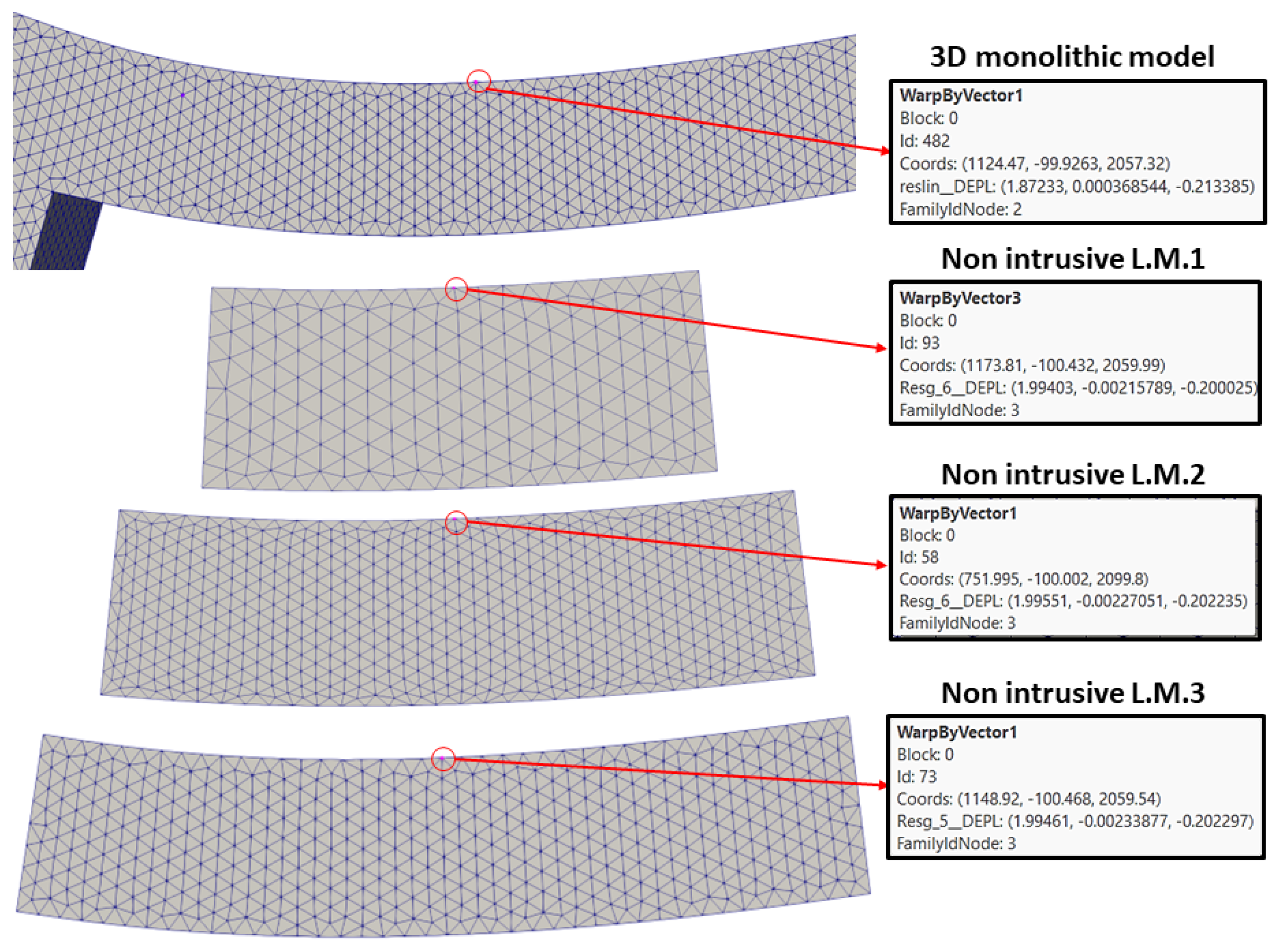
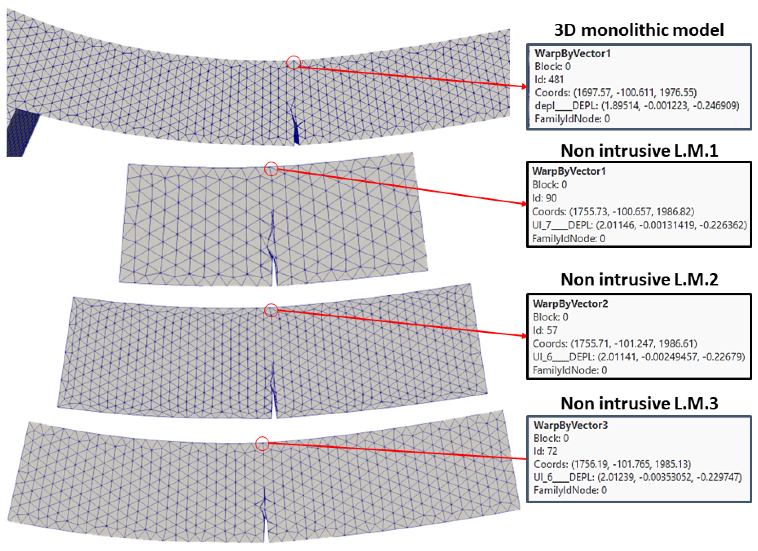
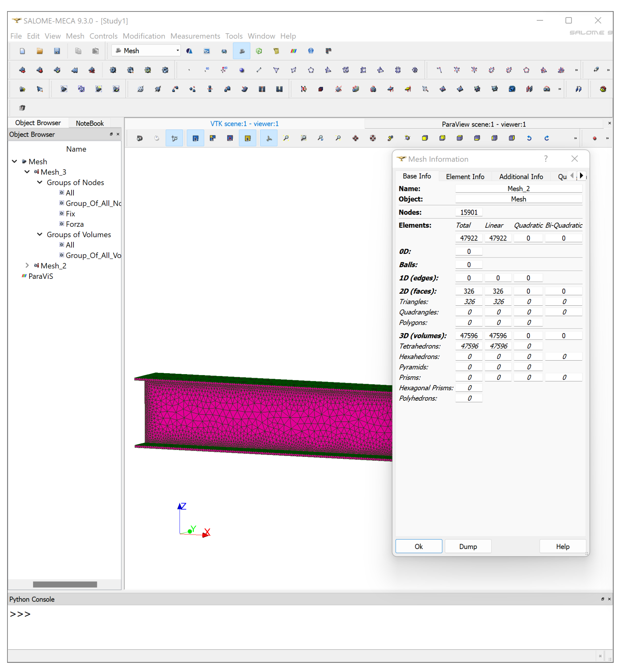
3.1. Validation of the Implementation in Code_Aster

In order to validate the procedure, the results of the non-intrusive global–local implementation are compared to a monolithic 3D solution of the problem, which considers the same properties of the crack location, number of propagation steps and also solved by means of the XFEM methodology. This analysis of the monolithic XFEM model allows us to do two things: to propagate the initialized crack in a model with a large number of degrees of freedom and also to compare the global–local methodology with a corresponding control model, obtaining displacement measurements and calculating errors between the mentioned methods. Figure 11 shows the graphical solution to the displacements obtained by the non-intrusive using a 1000 mm width local model, while Figure 12 presents the solution of the 3D monolithic problem, both with the same 50 mm crack.

Figure 13 shows the displacements for the 3D monolithic model (upper figure) and for the non-intrusive global–local methodology (lower figures) for the case of linear behavior and in Figure 14 the results are presented for the 50 mm crack, where the differences in the magnitude of the displacements in the 3 directions are relatively small respect to the size of the structure (3000 mm in wide and 2000 mm in height). In

Table 1. Non-intrusive norm displacement error analysis $Code\_Aster$ for different meshes and crack initial lengths.

Local Mesh Model		Initial Crack Length in the Local Model
		Linear	25 mm	50 mm	75 mm
Local Mesh 1	% disp. error	6.35%	5.96%	5.91%	non conv.
Local Mesh 2	% disp. error	6.44%	5.93%	5.91%	6.62%
Local Mesh 3	% disp. error	6.39%	5.95%	5.98%	6.44%

, the error with respect to the norm of the displacement of the monolithic model is presented for all models, being less than 6.7% for all converged cases.

It can be concluded that the error is independent of the crack propagation, i.e., the nonlinear behavior does not affect in terms of the error but is intrinsic to the global–local methodology and the transformation of displacements and forces between 1D and 3D models.

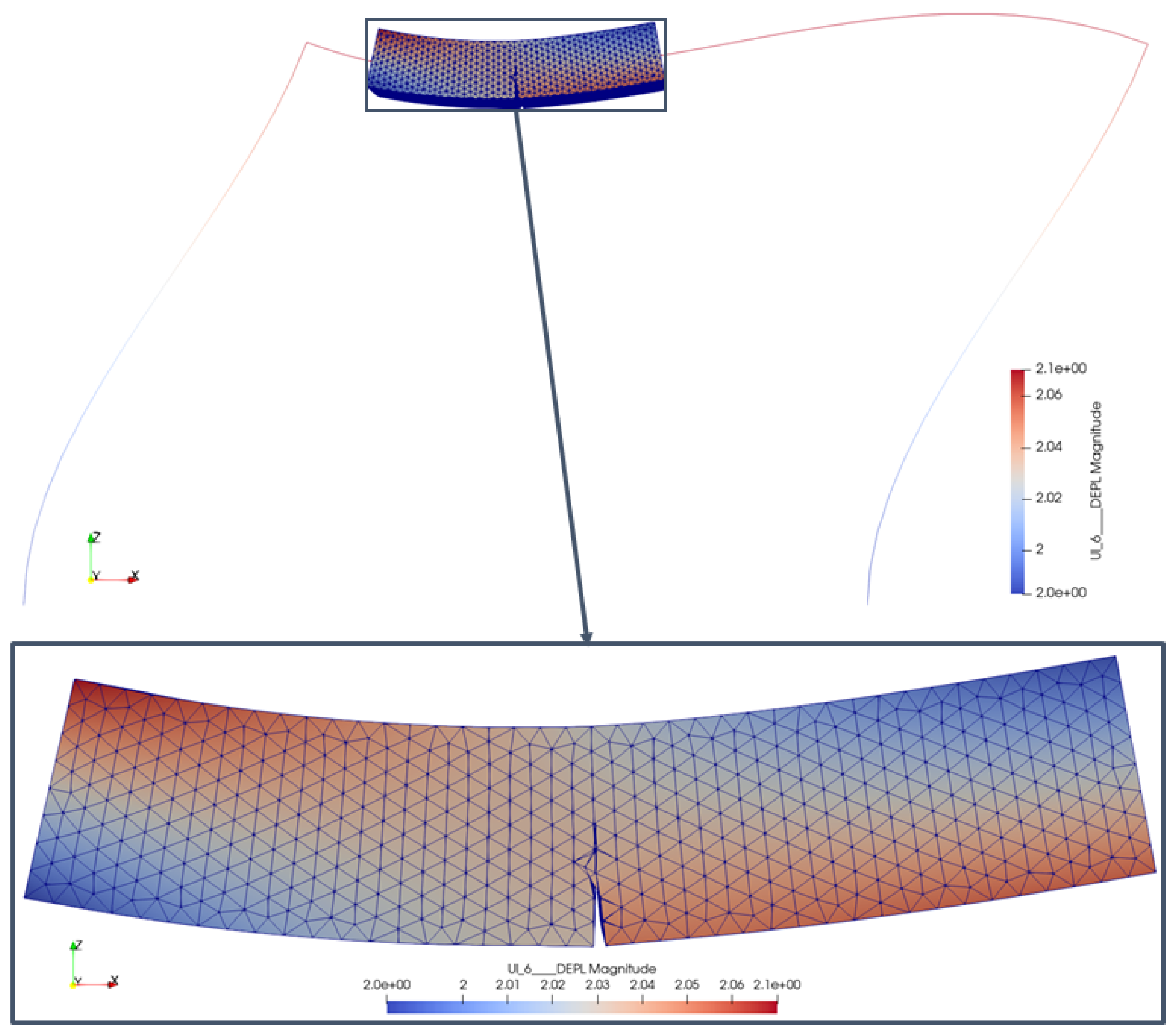
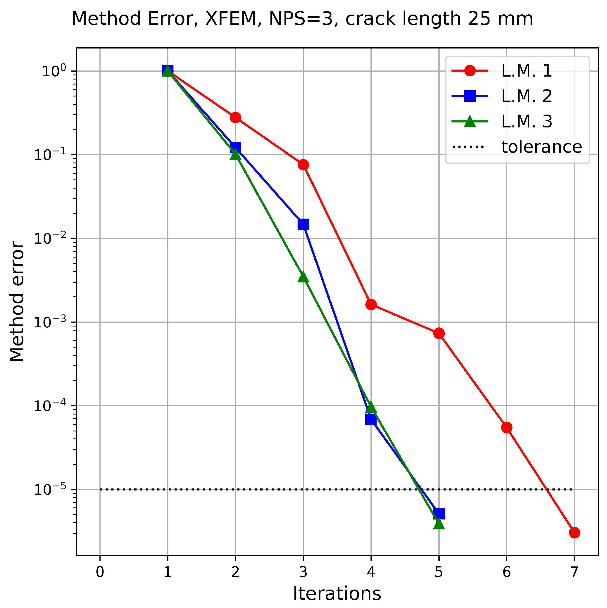
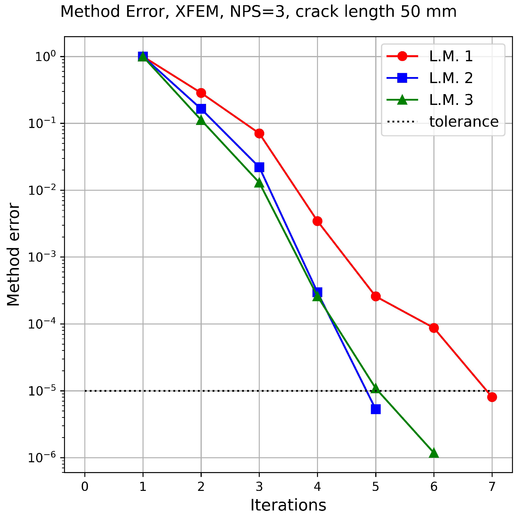
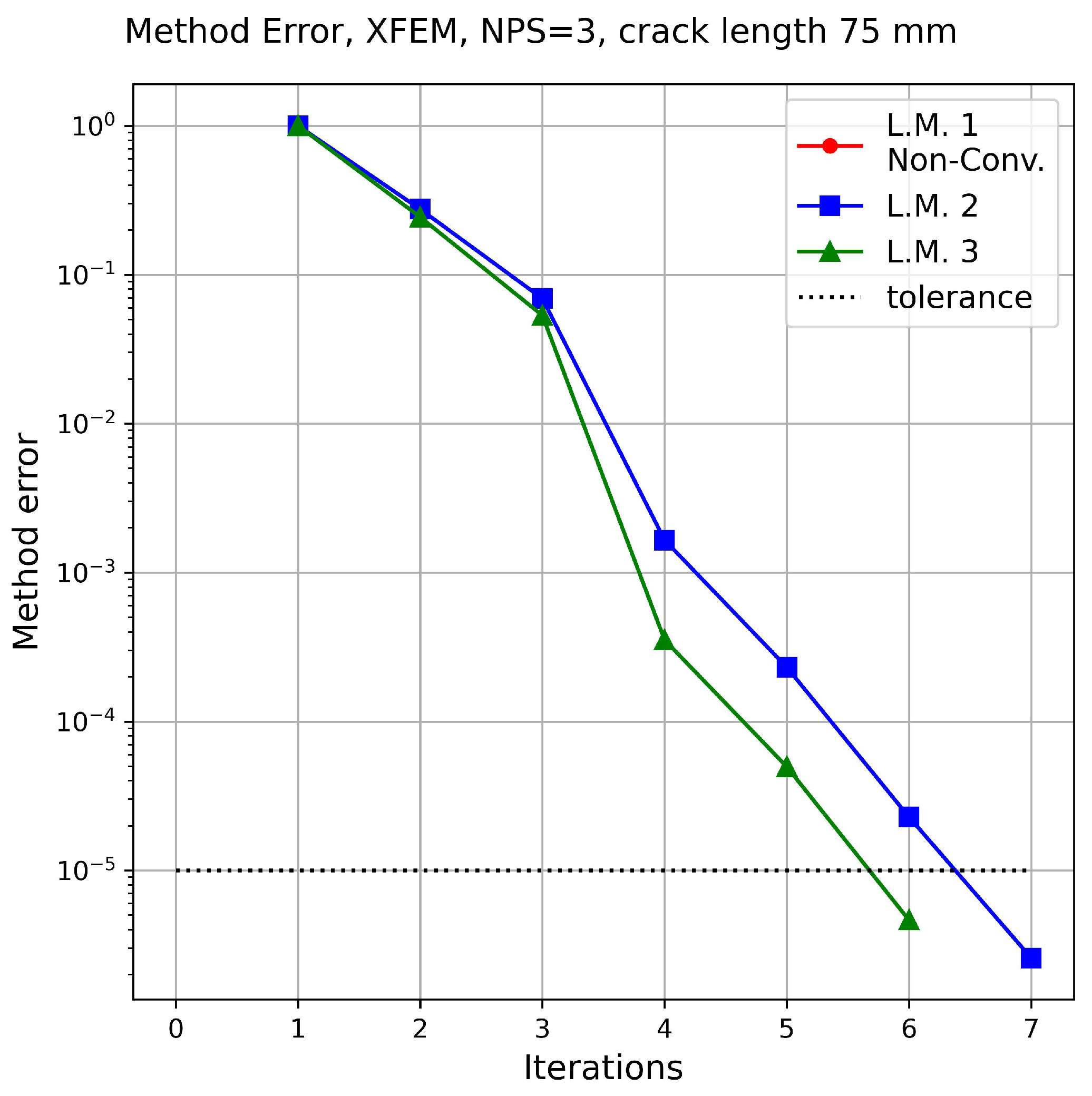
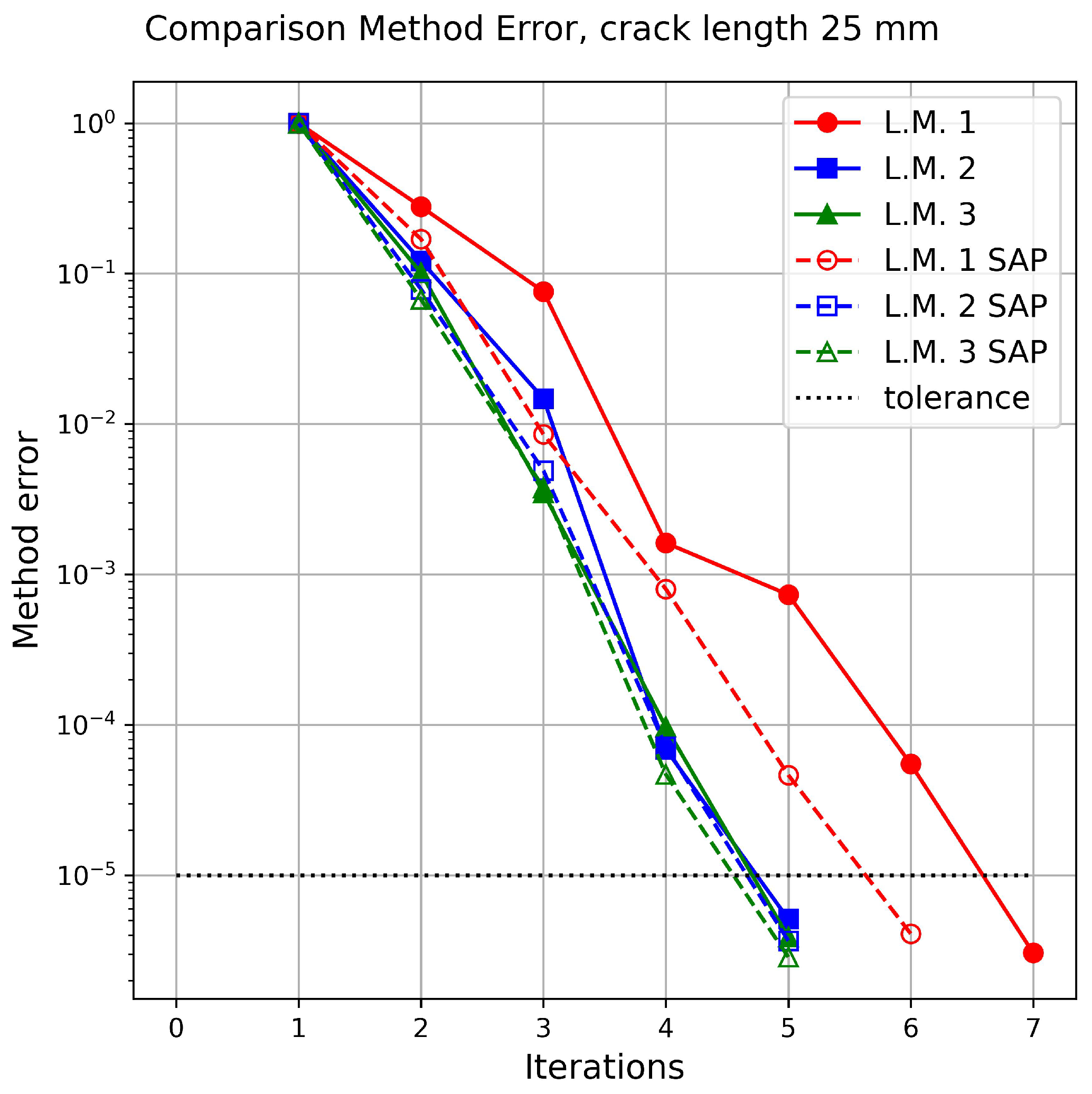
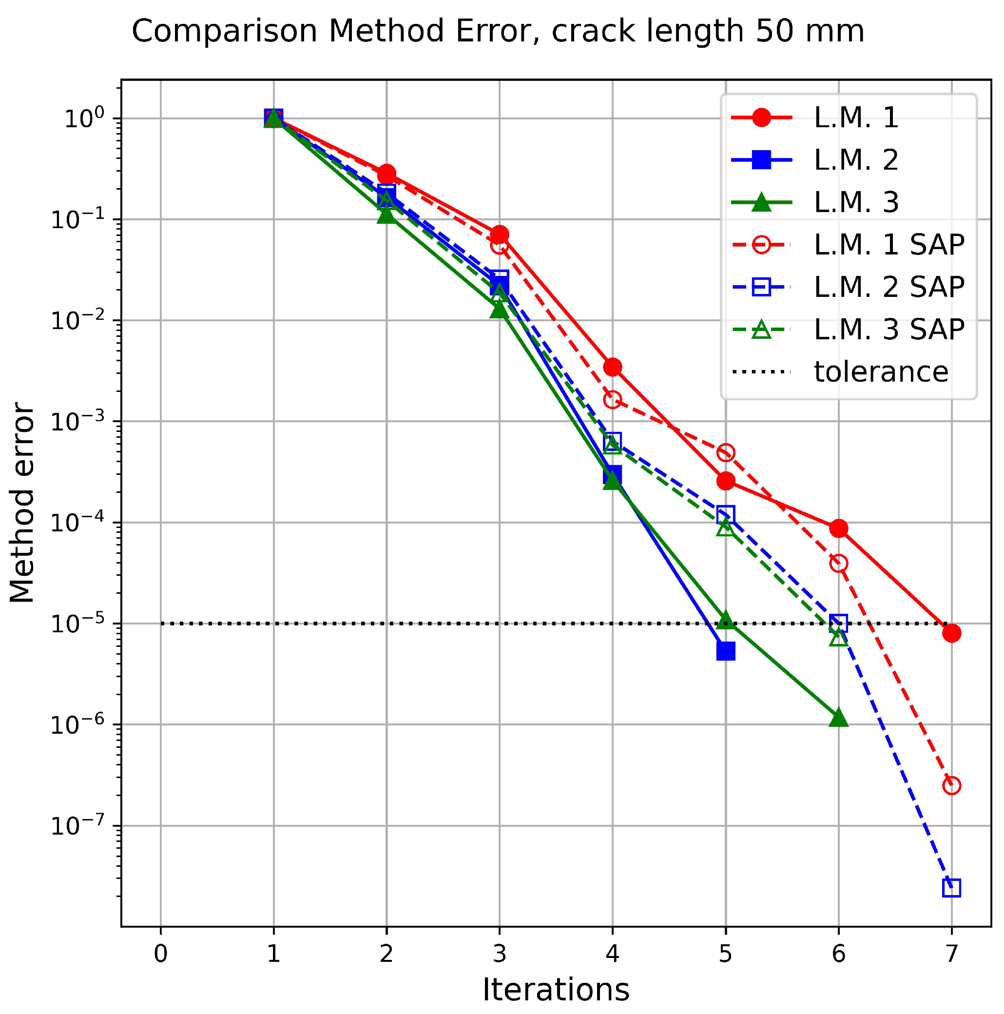
3.2. Effect of the Local Model Size

For the first analysis, no crack was considered on the model, in order to make it linear. Figure 15 shows the evolution of the error with respect to the number of iterations obtained for the different local models. It can be seen that as the size of the local problem increases, the convergence rate improves from seven iterations for the L.M.1 to five iterations for the L.M.3. It can be said that the length of the local model affects the convergence of the problem.

To analyze the effect of the size of the local model for non-linear cases, 3 crack lengths were considered: 25 mm, 50 mm and 75 mm. Figure 16, Figure 17 and Figure 18 shows the evolution of the error with respect to the number of iterations for the case of the crack of 25 mm, 50 mm and 75 mm, respectively.

It can be seen that L.M.2 and L.M.3 converge in a similar number of iterations giving a faster convergence rate than L.M.1, which required two more iterations on average or fails to converge (Figure 17).

With respect to the non-convergence of the L.M.1 analysis with 75 mm initial crack, there are two ways that the presented methodology considers this failed state:

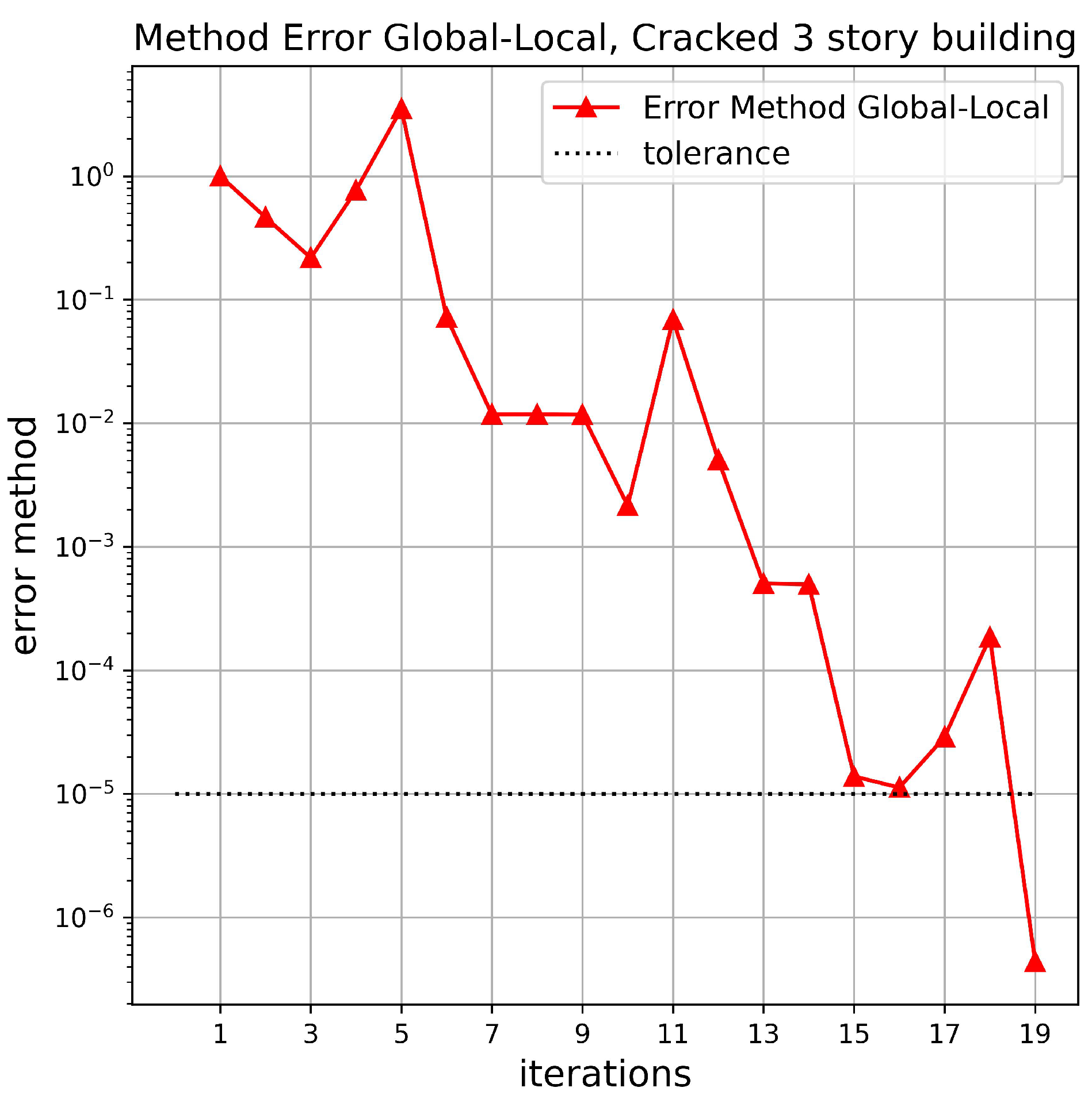
• Stagnation of the solution: If the iterative analysis presents a divergent error (increasing with each iteration), jumps between an error greater than the tolerance, or does not converge within a maximum number of iterations, i.e., 50 iterations in the present study.
• Failed crack propagation analysis (XFEM internal procedure): Crack propagation in Code_Aster is calculated using the rate of energy release (G) method, using the built-in function $CALC\_K\_G$. This method calculates the intensity stress factors (K) evaluating the bilinear form of G with the asymptotic solution of Westergaard. In addition, an error indicator is obtained by comparing the difference between G and Irwin’s energy release rate ($G_{Irwin}$), as shown in Equation (32) [46].

  $$\begin{array}{c}\hfill erro{r}_{XFEM}=\frac{\left|G-G_{Irwin}\right|}{\left|G\right|}\end{array}$$

  (32)
  If the error calculated using the Equation (32) is greater than 50%, the analysis stops and displays an alert message as presented in [46]. This is the case for the L.M.1 local mesh with the 75 mm initial crack length, affecting the convergence of XFEM method and, therefore, the overall convergence of the global–local analysis. More information with respect to the convergence of the XFEM crack propagation method can be found in [47,48].

Therefore, it is possible to conclude that for small local domains, the non-linearity effect does not fully develop before the interface, as postulated in St. Venant’s principle, generating problems in the coupling between the models.

4. Implementation with a Commercial Software

The selected software to test the non-intrusive strategy is SAP2000 [49], which is widely used for the analysis of reinforced concrete and steel structures. However, SAP 2000 does not have the capabilities to perform crack propagation, so it is proposed to couple the software with Code_Aster, using Python as an interface.

SAP2000 is a finite element program with an object-oriented 3D graphical interface, allowing to perform the modeling, analysis, and sizing of structural engineering problems. This software is used by engineers due to its versatility to model structures allowing to design of bridges, buildings, stadiums, dams, industrial structures, maritime structures, and generally all types of infrastructure that need to be analyzed and sized [49]. An important feature is that it solves simple static models that can be enriched with the non-intrusive methodology.

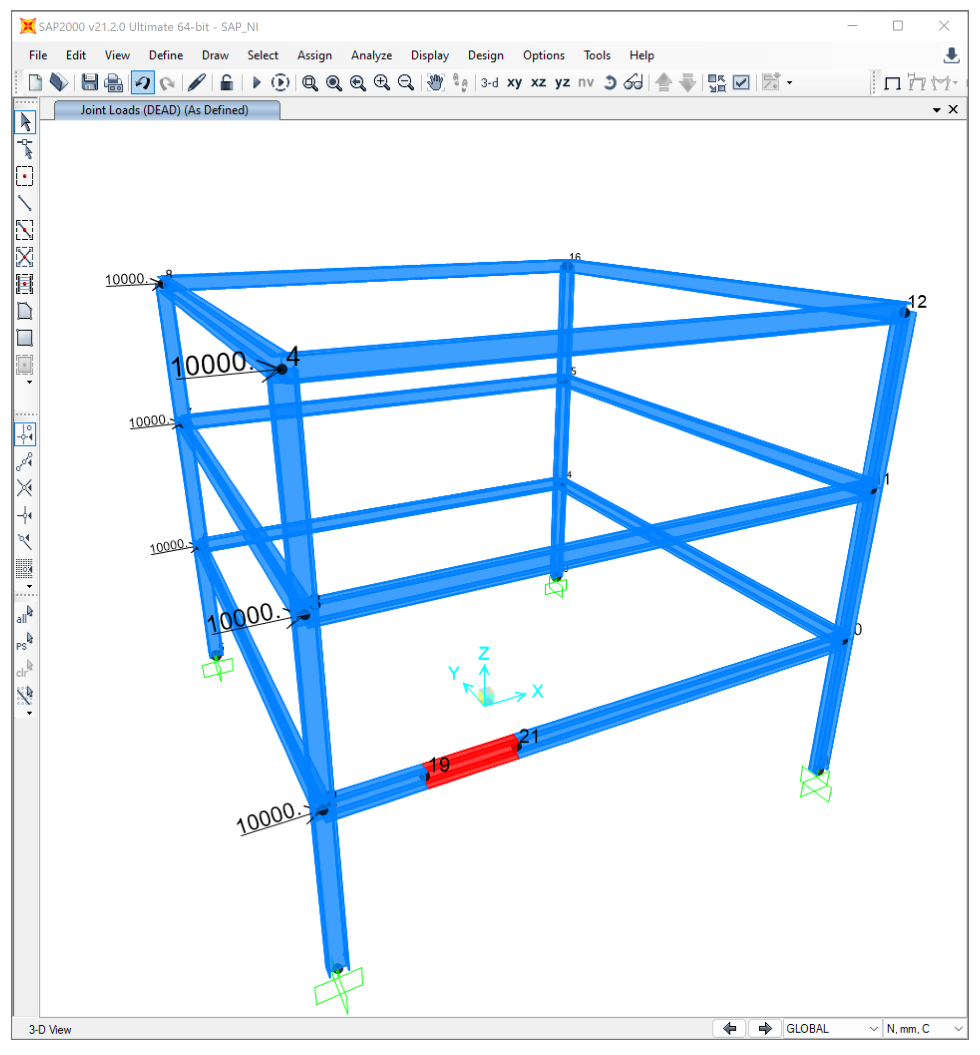
4.1. Validation of the Implementation in SAP 2000

The same structure analyzed in Section 3.1 is reviewed, with the same applied loads, sections and profiles to be analyzed. The SAP2000 model is shown in Figure 19.

To communicate SAP2000 with Code_Aster, the library comtypes is used, which allows information such as displacements and forces to be sent between different software using Python as an interpreter. The same cases and crack positions as the model analyzed in Code_Aster are analyzed to validate the methodology but using the commercial software for 1D linear calculation.

The results for the crack length of 25 mm, 50 mm and 75 mm are shown in Figure 20, Figure 21 and Figure 22, respectively. Solid lines correspond to the results of Section 3.1, while the dashed lines correspond to the implementation with SAP2000.

The error with respect to the norm of the displacement of the monolithic model is presented in

Table 2. Non-intrusive norm displacement error analysis coupling with SAP 2000, different meshes and crack initial lengths.

Local Mesh Model		Initial Crack Length in the Local Model
		Linear	25 mm	50 mm	75 mm
Local Mesh 1	% error disp.	8.94%	8.41%	8.32%	non conv.
Local Mesh 2	% error disp.	8.87%	8.33%	8.32%	9.11%
Local Mesh 3	% error disp.	8.79%	8.32%	8.37%	non conv.

, presenting an error lower than 9.2% for all converged cases. The magnitude of the displacements in the X and Z direction for both models are considered similar and the displacements in the Y direction are lower than 0.003 mm, and therefore are considered negligible.

As shown, the analysis with SAP 2000 for the case with L.M.1 and L.M.3 (for the initial crack of 75 mm) does not converge. As was presented in the previous section, these models failed to achieve a correct crack propagation analysis, and therefore, the XFEM stopped the global–local iterative procedure. Finally, the error is also independent of the nonlinear behavior analyzed and can be considered inherent to the global–local methodology.

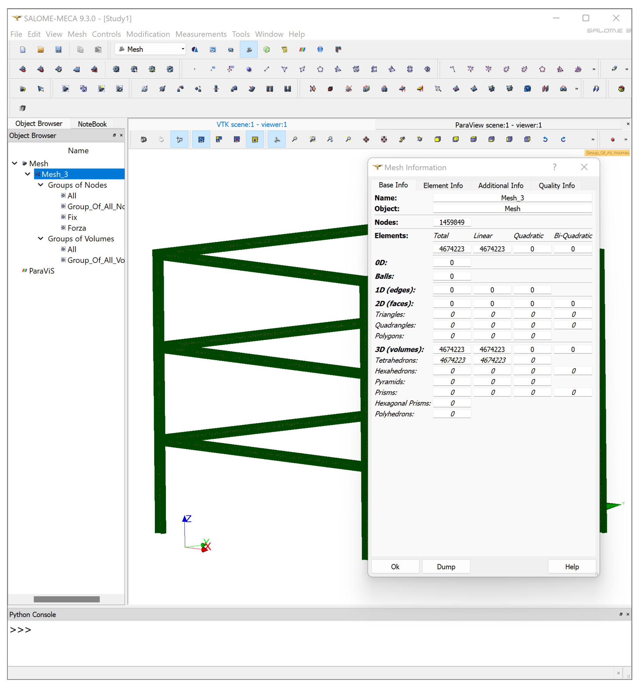
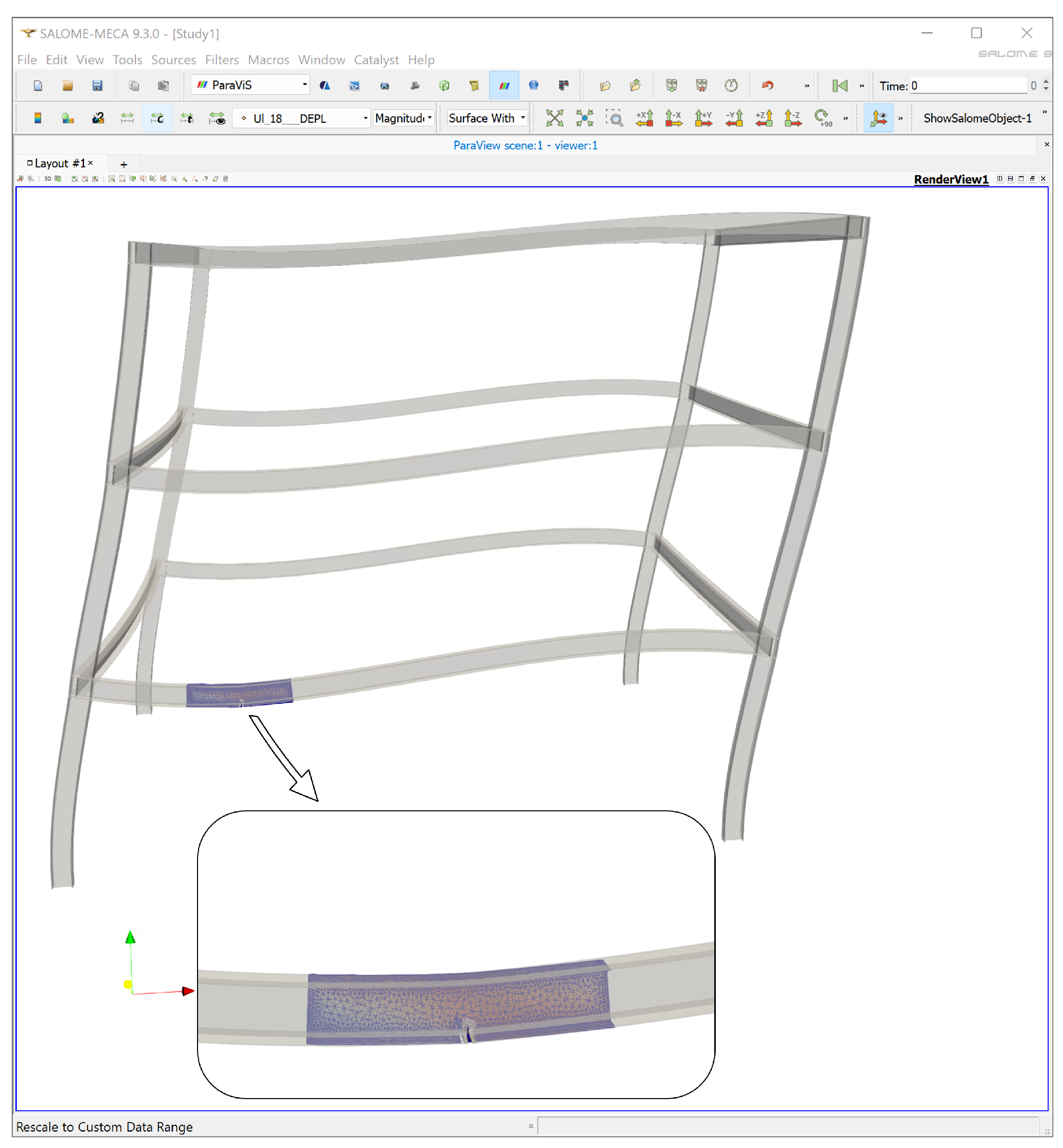
4.2. Methodology Extension to 3-Story Building

The building corresponds to a three-story steel structure with a height between floors of 3 m. The length of the span is 10 m in the X and Y directions. Forces of 10,000 N are applied to each corner of the building in the X direction considering rigid supports, where the local model is shown in red in Figure 23. The global 1D model consists of 18 nodes and 108 degrees of freedom.

The beams and columns correspond to Wide Flange profiles. The dimensions of the section are as follows:

• Total height: H = 300 mm.
• Flange width: B = 200 mm.
• Flange thickness: tf = 10 mm.
• Web thickness: tw = 6 mm.
• Material: Grade 50 quality steel.

The local problem, shown in Figure 24, is 1500 mm long, an initial crack length of 50 mm (centered on the local model), and three propagation steps.

The local model consists of 15,900 nodes and 47,703 degrees of freedom, modeled using tetrahedral elements. As a reference, a complete 3D modeling of the building in Salome Meca (Code_Aster Visual Interface) is considered, shown in Figure 25. This model has approximately 1,459,000 nodes, which implies 4,377,000 degrees of freedom.

Figure 26 shows in overlapping the displacements of the monolithic model (Code_Aster) and the local model (SAP2000).

The evolution of the error is presented in Figure 27.

Table 3. Results for 3D monolithic model and SAP 2000 global–local model.

Model	Crack Tip Displ. (mm)	Execution Time (s)
3D Monolithic	6.01	2231
GL w/SAP 2000	5.89	391
Diff. r/Monolithic	1.6%	82%

shows the magnitude in which the crack grows and the calculation time for each implementation. In addition, it indicates the percentage difference between the model in SAP2000 and Code_Aster. The results show that the growth of the crack, for both cases, is similar (difference of 1.6%). On the contrary, the calculation time is reduced by 82% for the non-intrusive case with SAP2000.

It is expected that for the analysis of much larger structures (multiple-story buildings) the size of the local problem does not vary, but the global problem does. Being the global problem the one with the least number of nodes and d.o.f., this should not have a significant influence on the computation times for the non-intrusive problem, but it would mean a significant increase for the monolithic case.

5. Discussion

Non-intrusive global–local analysis with 1D to 3D coupling is a technique that allows a localized analysis of a problem which, in the framework of this work, was crack propagation, but can also be used regarding plasticity, crystalline plasticity, stress concentrations, etc.

The implementation that was developed allows us to consider the displacements in the six degrees of freedom of the global model and the three degrees of freedom of the local model, having a kinematic compatibility in the transfer of the displacements and subsequent compensation of forces.

The dimensions of the local model and the crack location affect the number of iterations required to obtain convergence. Despite this, it was possible to verify displacements obtained using the methodology through the displacements, resulting in low errors relative to the monolithic model.

This methodology was implemented in a test model and was the first step in the analysis of large civil structures (buildings, bridges, etc.) that present non-linearities. The correct implementation in larger cases would save costs without losing accuracy in the computational solution, since the degrees of freedom to be studied are significantly reduced considering that in the case study, the discretization of the structure was reduced from 3500 elements to about 250.

The non-intrusive global–local analysis with 1D to 3D coupling presented a displacement error of 10% according to the tolerance used, showing good primal–dual compatibility. However, there may also be cases of higher stiffness structures, so mixed coupling can be used to improve compatibility. In addition, the ideal dimensions of the local model can be determined according to the crack location and thus verify the methodology obtaining the energy release rate.

The methodology used was verified through the commercial software SAP 2000, obtaining a similar number of iterations to convergence with respect to those obtained using Code_Aster applying it to a 3-story building, significantly reducing the execution time with an acceptable error. This result opens up the possibility to extend this methodology to the industry and use it in practical applications.

This work is limited to monotonic loads in order to study the effect of the non-intrusive methodology for crack propagation in 1D global models to 3D local models. As shown in the results presented of the different problems analyzed, the error is low and maintained for the different cases investigated. Therefore, for future research, the study of sequential loading for crack propagation could be studied in order to verify the effect of nonlinear 1D structures with localized cracks and also to study the effect on the development of the crack for this type of loads. Another topic to consider is to analyze more section types, lengths of the local model, and crack location, in order to present in future studies a criterion to decide the length of the local model that optimizes the global–local non-intrusive analysis, given the properties of the problem. Finally, as was presented in this study, the crack propagation was analyzed considering only steel frame elements. Nevertheless, other materials and specific nonlinear behavior could be studied, such as the total crack strain model for reinforced concrete local models.

References

- AISC Committee. Specification for Structural Steel Buildings (ANSI/AISC 360-10); American Institute of Steel Construction: Chicago, IL, USA, 2010. [Google Scholar]
- AISC Committee. Seismic Provision for Structural Steel Buildings (ANSI/AISC 341-16); American Institute of Steel Construction: Chicago, IL, USA, 2016. [Google Scholar]
- Frangopol, D.M.; Soliman, M. Life-cycle of structural systems: Recent achievements and future directions. Struct. Infrastruct. Eng. 2019, 12, 46–65. [Google Scholar]
- Cui, W. A state-of-the-art review on fatigue life prediction methods for metal structures. J. Mar. Sci. Technol. 2002, 7, 43–56. [Google Scholar] [CrossRef]
- Moës, N.; Dolbow, J.; Belytschko, T. A finite element method for crack growth without remeshing. Int. J. Numer. Methods Eng. 1999, 46, 131–150. [Google Scholar] [CrossRef]
- Belytschko, T.; Black, T. Elastic crack growth in finite elements with minimal remeshing. Int. J. Numer. Methods Eng. 1999, 45, 601–620. [Google Scholar] [CrossRef]
- Khoei, A.R. Extended Finite Element Method: Theory and Applications; John Wiley & Sons: New York, NY, USA, 2014. [Google Scholar]
- Erkmen, R.E.; Saleh, A.; Afnani, A. Incorporating local effects in the predictor step of the iterative global-local analysis of beams. Int. J. Multiscale Comput. Eng. 2016, 14, 455–477. [Google Scholar] [CrossRef]
- Valipour, H.R.; Foster, S.J. Nonlocal Damage Formulation for a Flexibility-Based Frame Element. J. Struct. Eng. 2009, 135, 1213–1221. [Google Scholar] [CrossRef]
- Roux, F.X. Method of finite element tearing and interconnecting and its parallel solution algorithm. Int. J. Numer. Methods Eng. 1991, 32, 1205–1227. [Google Scholar]
- Pebrel, J.; Rey, C.; Gosselet, P. A Nonlinear Dual-Domain Decomposition Method: Application to Structural Problems with Damage. Int. J. Multiscale Comput. Eng. 2008, 6, 251–262. [Google Scholar] [CrossRef]
- Hinojosa, J.; Allix, O.; Guidault, P.A.; Cresta, P. Domain decomposition methods with nonlinear localization for the buckling and post-buckling analyses of large structures. Adv. Eng. Softw. 2014, 70, 13–24. [Google Scholar] [CrossRef]
- Guidault, P.A. Une Stratégie de Calcul pour les Structures Fissurées: Analyse Locale-Globale et Approche Multiéchelle Pour la Fissuration. Ph.D. Thesis, École Normale Supérieure de Cachan-ENS Cachan, Gif-sur-Yvette, France, 2007. [Google Scholar]
- Kerfriden, P.; Allix, O.; Gosselet, P. A three-scale domain decomposition method for the 3D analysis of debonding in laminates. Comput. Mech. 2009, 44, 343–362. [Google Scholar] [CrossRef]
- Oumaziz, P.; Gosselet, P.; Boucard, P.A.; Guinard, S. A non-invasive implementation of a mixed domain decomposition method for frictional contact problems. Comput. Mech. 2017, 60, 797–812. [Google Scholar] [CrossRef]
- Allix, O.; Gosselet, P. Non intrusive global/local coupling techniques in solid mechanics: An introduction to different coupling strategies and acceleration techniques. In Modeling in Engineering Using Innovative Numerical Methods for Solids and Fluids; Springer: Berlin/Heidelberg, Germany, 2020; pp. 203–220. [Google Scholar]
- Whitcomb, J.D. Iterative global/local finite element analysis. Comput. Struct. 1991, 40, 1027–1031. [Google Scholar] [CrossRef]
- Gendre, L.; Allix, O.; Gosselet, P.; Comte, F. Non-intrusive and exact global/local techniques for structural problems with local plasticity. Comput. Mech. 2009, 44, 233–245. [Google Scholar] [CrossRef]
- Duval, M.; Passieux, J.C.; Salaün, M.; Guinard, S. Non-intrusive Coupling: Recent Advances and Scalable Nonlinear Domain Decomposition. Arch. Comput. Methods Eng. 2016, 23, 17–38. [Google Scholar] [CrossRef]
- Gosselet, P.; Blanchard, M.; Allix, O.; Guguin, G. Non-invasive global–local coupling as a Schwarz domain decomposition method: Acceleration and generalization. Adv. Model. Simul. Eng. Sci. 2018, 5, 4. [Google Scholar] [CrossRef]
- Fuenzalida-Henriquez, I.; Oumaziz, P.; Castillo-Ibarra, E.; Hinojosa, J. Global-Local non intrusive analysis with robin parameters: Application to plastic hardening behavior and crack propagation in 2D and 3D structures. Comput. Mech. 2022, 69, 965–978. [Google Scholar] [CrossRef]
- EDF. Code Aster, Analysis of Structures and Thermomechanics for Studies and Research; Électricité de France: Paris, France, 2019. [Google Scholar]
- Nayak, C.B.; Thakare, S.B. Seismic performance of existing water tank after condition ranking using non-destructive testing. Int. J. Adv. Struct. Eng. 2019, 11, 395–410. [Google Scholar] [CrossRef]
- dos Santos, R.B.; Tamayo, J.L.P. Coupling SAP 2000 with ABC algorithm for truss optimization. DYNA 2020, 87, 102–111. [Google Scholar] [CrossRef]
- Zandi, N.; Adlparvar, M.R.; Javan, A.L. Evaluation on Seismic Performance of Dual Steel Moment-Resisting Frame with Zipper Bracing System Compared to Chevron Bracing System Against Near-Fault Earthquakes. J. Rehabil. Civ. Eng. 2021, 9, 1–25. [Google Scholar] [CrossRef]
- Tampubolon, S.P.; Mulyani, A.S. Analysis and calculation of wooden framework structure by using Structural Analysis Program (SAP)-2000 and method of joint. IOP Conf. Ser. Earth Environ. Sci. 2021, 878, 012042. [Google Scholar] [CrossRef]
- Zhang, Y.; Madenci, E.; Zhang, Q. ANSYS implementation of a coupled 3D peridynamic and finite element analysis for crack propagation under quasi-static loading. Eng. Fract. Mech. 2022, 260, 108179. [Google Scholar] [CrossRef]
- Fageehi, Y.A. Fatigue Crack Growth Analysis with Extended Finite Element for 3D Linear Elastic Material. Metals 2021, 11, 397. [Google Scholar] [CrossRef]
- Alshoaibi, A.M.; Fageehi, Y.A. 3D modelling of fatigue crack growth and life predictions using ANSYS. Ain Shams Eng. J. 2022, 13, 101636. [Google Scholar] [CrossRef]
- Su, X.; Yang, Z.; Liu, G. Finite Element Modelling of Complex 3D Static and Dynamic Crack Propagation by Embedding Cohesive Elements in Abaqus. Acta Mech. Solida Sin. 2010, 23, 271–282. [Google Scholar] [CrossRef]
- Molnár, G.; Gravouil, A.; Seghir, R.; Réthoré, J. An open-source Abaqus implementation of the phase-field method to study the effect of plasticity on the instantaneous fracture toughness in dynamic crack propagation. Comput. Methods Appl. Mech. Eng. 2020, 365, 113004. [Google Scholar] [CrossRef]
- Távara, L.; Moreno, L.; Paloma, E.; Mantič, V. Accurate modelling of instabilities caused by multi-site interface-crack onset and propagation in composites using the sequentially linear analysis and Abaqus. Compos. Struct. 2019, 225, 110993. [Google Scholar] [CrossRef]
- Gontarz, J.; Podgórski, J. Comparison of Various Criteria Determining the Direction of Crack Propagation Using the UDMGINI User Procedure Implemented in Abaqus. Materials 2021, 14, 3382. [Google Scholar] [CrossRef]
- Navidtehrani, Y.; Betegón, C.; Martínez-Pañeda, E. A simple and robust Abaqus implementation of the phase field fracture method. Appl. Eng. Sci. 2021, 6, 100050. [Google Scholar] [CrossRef]
- Noii, N.; Aldakheel, F.; Wick, T.; Wriggers, P. An adaptive global–local approach for phase-field modeling of anisotropic brittle fracture. Comput. Methods Appl. Mech. Eng. 2020, 361, 112744. [Google Scholar] [CrossRef]
- Passieux, J.C.; Réthoré, J.; Gravouil, A.; Baietto, M.C. Local / global non-intrusive crack propagation simulation using a multigrid X-FEM solver. Comput. Mech. 2013, 52, 1381–1393. [Google Scholar] [CrossRef]
- Blanchard, M.; Allix, O.; Gosselet, P.; Desmeure, G. Space/time global/local noninvasive coupling strategy: Application to viscoplastic structures. Finite Elem. Anal. Des. 2019, 156, 1–12. [Google Scholar] [CrossRef]
- El Kerim, A.; Gosselet, P.; Magoulès, F. Asynchronous global–local non-invasive coupling for linear elliptic problems. Comput. Methods Appl. Mech. Eng. 2023, 406, 115910. [Google Scholar] [CrossRef]
- Magoulès, F.; Gbikpi-Benissan, G. JACK: An asynchronous communication kernel library for iterative algorithms. J. Supercomput. 2017, 73, 3468–3487. [Google Scholar] [CrossRef]
- Negrello, C.; Gosselet, P.; Rey, C. A new impedance accounting for short- and long-range effects in mixed substructured formulations of nonlinear problems. Int. J. Numer. Methods Eng. 2018, 114, 675–693. [Google Scholar] [CrossRef]
- Gendre, L.; Allix, O.; Gosselet, P. A two-scale approximation of the Schur complement and its use for non-intrusive coupling. Int. J. Numer. Methods Eng. 2011, 87, 889–905. [Google Scholar] [CrossRef]
- Peña, L.; Hinojosa, J. Implementation of a new expression for the search direction in simulations of structures with buckling and post-buckling: “Two-Scale Impedance”. J. Comput. Appl. Math. 2022, 403, 113799. [Google Scholar] [CrossRef]
- Aldakheel, F.; Noii, N.; Wick, T.; Wriggers, P. A global–local approach for hydraulic phase-field fracture in poroelastic media. Comput. Math. Appl. 2021, 91, 99–121. [Google Scholar] [CrossRef]
- Crisfield, M.A. A Fast Incremental/Iterative Solution Procedure That Handles “Snap-Through”; Computers and Structures: Walnut Creek, CA, USA, 1981. [Google Scholar] [CrossRef]
- Oñate, E. Structural Analysis with the Finite Element Method Linear Statics; Lecture Notes on Numerical Methods in Engineering and Sciences; Springer: Dordrecht, The Netherlands, 2013. [Google Scholar] [CrossRef]
- EDF. Code Aster, Manuel d’Utilisation Opérateur CALC G; Électricité de France: Paris, France, 2019. [Google Scholar]
- Lan, M.; Waisman, H.; Harari, I. A direct analytical method to extract mixed-mode components of strain energy release rates from Irwin’s integral using extended finite element method. Int. J. Numer. Methods Eng. 2013, 95, 1033–1052. [Google Scholar] [CrossRef]
- Sun, C.T.; Wang, C.Y. A new look at energy release rate in fracture mechanics. Int. J. Fract. 2002, 113, 295–307. [Google Scholar] [CrossRef]
- Computers & Structures, Inc. SAP2000, Modelado y Calculo de Estructuras a Traves de Elementos Finitos; Computers & Structures, Inc.: Walnut Creek, CA, USA, 2022. [Google Scholar]