Optimized-Weighted-Speedy Q-Learning Algorithm for Multi-UGV in Static Environment Path Planning under Anti-Collision Cooperation Mechanism

Abstract

With the accelerated development of smart cities, the concept of a “smart industrial park” in which unmanned ground vehicles (UGVs) have wide application has entered the industrial field of vision. When faced with multiple tasks and heterogeneous tasks, the task execution efficiency of a single UGV is inefficient, thus the task planning research under multi-UGV cooperation has become more urgent. In this paper, under the anti-collision cooperation mechanism for multi-UGV path planning, an improved algorithm with optimized-weighted-speedy Q-learning (OWS Q-learning) is proposed. The slow convergence speed of the Q-learning algorithm is overcome to a certain extent by changing the update mode of the Q function. By improving the selection mode of learning rate and the selection strategy of action, the relationship between exploration and utilization is balanced, and the learning efficiency of multi-agent in complex environments is improved. The simulation experiments in static environment show that the designed anti-collision coordination mechanism effectively solves the coordination problem of multiple UGVs in the same scenario. In the same experimental scenario, compared with the Q-learning algorithm and other reinforcement learning algorithms, only the OWS Q-learning algorithm achieves the convergence effect, and the OWS Q-learning algorithm has the shortest collision-free path for UGVS and the least time to complete the planning. Compared with the Q-learning algorithm, the calculation time of the OWS Q-learning algorithm in the three experimental scenarios is improved by 53.93%, 67.21%, and 53.53%, respectively. This effectively improves the intelligent development of UGV in smart parks.

1. Introduction

The general trend of the fourth revolution is intelligence, which is characterized by the integration of wisdom into the physical system of real objects, and one of its technical trends is intelligent complex systems, artificial intelligence, and smart cities [1]. A smart industrial park is an important manifestation of a smart city, with the enrichment of intelligent scenes and the continuous evolution of industrial park forms, the functions carried by the industrial park are becoming increasingly diversified and three-dimensional, and with the development of the smart industrial park, the path planning of unmanned vehicles in the industrial park has also attracted widespread attention from scholars. Although the method of path planning is mature, due to the complex environment, irregular road lines, large areas of the industrial park, and large flow of people, it is still challenging for unmanned vehicles to carry out path planning in the industrial park. At the present stage, due to the slow speed and safety of unmanned vehicles in the industrial park, they have shown great advantages in research and application. Therefore, the study of unmanned vehicles in industrial park path planning has high research value and practical application significance.

An unmanned ground vehicle (UGV) is an artificially remote-controlled, semi-autonomous, or autonomous agent that can replace humans in performing diverse and high-risk tasks and plays an important role in many practical applications [2]. Due to the increased demand, the simultaneous coordinated use of a group of vehicles in order to perform tasks more efficiently has aroused the interest of scholars [3]. Compared with a single UGV, multiple UGVs can perform tasks in parallel and cover a larger area, and the system can continue to work even if one robot fails [4]. The simultaneous use of multiple UGVs at the same time can effectively shorten the time of task execution and improve the efficiency of task execution, but it also increases the complexity of planning to a certain extent [5]. Due to the high computational complexity of multi-agent path planning, there is a lack of complete algorithms that provide solution optimization and computational efficiency [6].

With the growing interest in intelligent assistive technologies and autonomous robotic vehicles, path planning has become one of the most challenging topics in the field of navigation research [7]. Path planning is divided into offline planning and online planning [8]. When generating paths for multi-agents, the multi-agents under offline planning cannot take advantage of the cooperation capability due to no or little interaction between them, and finally, the multi-agent system cannot ensure that the robot walks along the predetermined path, and when generating paths for multi-agent online planning, there is often a certain interaction among multiple agents [8]. For the solution of some complex problems, sometimes some strategies need to be adopted. For example, Liao et al. [9] proposed a channel-related payload division strategy based on channel modification probability to solve the problem of how to use inter-channel correlation to allocate payload to enhance color image performance. The interaction among multiple agents is manifested in the cooperation strategy among agents, which is divided into centralized and decentralized. Centralized systems are more cooperative than decentralized systems because they have a central decision-maker, where the central decision-maker assigns tasks and schedules to each agent [10]. Although centralized decision-making has no restrictions on the algorithms used to solve problems, in general, decentralized decision-making is more widely used in practice, which enables agents to communicate and interact with each other, reduces the computational complexity through limited sharing of information, and has higher flexibility, robustness, and scalability [10].

The most commonly used method of path planning is the heuristic algorithm, but when the solution conditions involved are more complex, the traditional heuristic algorithm is inefficient, so many scholars use improved heuristic algorithms to solve path planning problems. Zhang et al. [11] proposed an improved A* algorithm including two-way sector expansion and variable-step search strategy for complex terrain and static radar threats in order to quickly avoid static threats. Saranya et al. [12] proposed an improved D* algorithm for the path planning problem of complex environments, introducing terrain slope into cost function calculation. Guo et al. [13] proposed a chaotic shared learning particle swarm optimization algorithm (CSPSO) for the path planning and path control problem of USV with multi-objective constraints.

However, in the face of changing environments, classical path planning algorithms can no longer meet the real-time and efficient requirements of path planning, so more and more reinforcement learning algorithms are used to solve agent path planning problems. Reinforcement learning is an algorithm that finds the best solution through trial and error in an unknown environment, and reinforcement learning is widely used in path planning because of its own characteristics. In addition, reinforcement learning is also used to solve problems such as image steganography and other problems, and Tan et al. [14] proposed a new end-to-end network architecture based on GAN for image steganism. As a model-free algorithm in reinforcement learning algorithms, the goal of the Q-learning algorithm is to learn a strategy that can handle random transformation and reward problems without adapting to the environment. Q-learning algorithms are widely used because of their simplicity and easy convergence, but Q-learning algorithms also have some shortcomings in reinforcement learning. In recent years, some scholars have proposed some improved Q-learning algorithms for the shortcomings of the Q-learning algorithm. Hu et al. [15] proposed a multi-agent Q-learning method NashQ in the framework of general and random games, which guarantees convergence considering some highly restrictive assumptions about the stage game form during the learning process, and its advantage is that the complexity is relatively low. In order to overcome the inefficiency of the basic Q-learning algorithm in multi-agent systems, Ono et al. [16] proposed the modular Q-learning algorithm, which decomposes the big problem to be learned into small problems and applies Q-learning to each sub-problem. Using basic Q-learning algorithms in multi-agent environments, where agents are often unable to find answers or take a lot of time to solve problems, Iima et al. [17] proposed a group reinforcement learning algorithm based on the Sarsa method to quickly obtain the optimal strategy for the maximum reward problem. Low et al. [18] introduced the concept of partially guided Q-learning and initialized the Q table using the pollination algorithm (FPA). Li et al. [19] proposed a dynamic parameter adjustment strategy and an action deletion mechanism of trial and error method on the basis of Q-learning combined with $\epsilon -greedy$, so as to better balance the relationship between exploration and utilization and improve the exploration efficiency of the agent. The above research has made useful progress in improving the efficiency of Q-learning algorithms, however, in large and complex environments, Q-learning algorithms are difficult to achieve the desired results.

Therefore, in order to promote the intelligent development of smart parks, give full play to the advantages of unmanned vehicles in global path planning and obstacle avoidance. In view of the low efficiency of single UGV task execution and blind exploration of UGVS random selection of actions under Q-learning algorithm in complex environments, resulting in low learning efficiency, slow convergence speed in complex environments, this paper proposes an improved Q-learning algorithm to solve the path planning problem of multi-UGV based on the idea of Q-learning algorithm and distributed collaboration strategy between multiple agents. The algorithm expects to obtain better path planning results than the traditional Q-learning algorithm, which can enable multiple UGVs to find their respective paths in the same iteration, reduce the time of path planning, and obtain a shorter final path. The specific improvement of the Q-learning algorithm in this paper is to change the update method of the Q function, use a more aggressive learning rate to accelerate the convergence speed of the algorithm, and select actions more effectively by improving the $\epsilon -greedy$ strategy. The main contributions of this paper are as follows:

• Aiming at the problem of path planning of multiple UGVs in the complex environment of smart parks, a grid environment model is established, and an anti-collision coordination mechanism between multiple UGVs is proposed.
• Aiming at the problem that the Q-learning algorithm converges slowly in the complex environment of multi-agent systems, the Q estimate of the next state and the Q value of the current state is weighted to change the update mode of the Q function, so as to overcome the problem of slow convergence speed of the Q-learning algorithm. By using a more aggressive learning rate and a ε − greedy strategy with improved action selection, the relationship between exploration and utilization of the Q-learning algorithm is balanced, the convergence speed of the algorithm is accelerated, and an improved reinforcement learning algorithm optimized-weighted-speedy Q-learning (OWS Q-learning) algorithm is proposed.
• The proposed algorithm is compared with the SARSA algorithm, Q-learning algorithm, and speedy Q-learning algorithm, the comprehensive performances of stability and robustness of the proposed algorithm are explained from the evaluation indexes such as shortest path steps, path length, calculation time, and reward function convergence.

The rest of this article is organized as follows. In Section 2, the literature related to multi-agent autonomous path planning is briefly summarized. In Section 3, a simulation environment model is established, and the collision avoidance cooperation mechanism in multi-UGV path planning and evaluation indexes of the algorithm are introduced. In Section 4, the theory of reinforcement learning and the proposed improved algorithm are introduced. In Section 5, the experimental scenario and experimental parameters are set, the simulation experiments are carried out, and the experimental results are compared and analyzed. In Section 6, the full text is summarized and an outlook for future work is provided.

2. Related Work

Path planning algorithms are widely used in indoor and outdoor path planning problems, and so far, scholars have conducted a lot of research on path planning problems, and various methods have been proposed to better solve path planning problems [8]. Multi-robot path planning algorithms can be divided into three categories: classical algorithms, heuristic algorithms, and artificial intelligence algorithms [3].

Among the classical algorithms, Zhao et al. [20] proposed a collision avoidance strategy and risk assessment based on improved APF and fuzzy inference systems for multi-robot path planning in completely unknown environments. Yu [21] aimed at the optimal multi-robot path planning problem with computational complexity and used the floor plan to establish the complexity of the problem on the floor plan to reduce path sharing in the opposite direction. Alottaibi et al. [22] argued that for multi-robot path planning problems, the RRT algorithm outperforms the Bibox algorithm in optimizing solutions and exploring search spaces in urban environments. Nedjati et al. [23] proposed a centralized algorithm framework for the multi-robot path planning problem in general two-dimensional continuous environment, which obtained a high level of effectiveness by discretizing the continuous environment and quickly solving the resulting discrete planning problem. Dutta et al. [24] aimed at the NP difficulty problem of multi-robot path planning under communication constraints, using continuous region division into Voronoi components to effectively divide initially unknown environments among robots according to newly discovered obstacles, thereby improving load balancing among robots. Yuan et al. [25] proposed a two-layer path planning algorithm—an improved A* algorithm and a dynamic fast exploration random tree (RRT) algorithm with kinematic constraints to optimize the path of multiple AGVs, and simulation experiments show that the proposed two-layer path planning algorithm performs well in search efficiency and significantly reduces the incidence of multiple AGV path conflicts. Singh et al. [26] proposed the EA* algorithm, allocation technology, and fault detection algorithm using the circumferential division method for the target location-allocation problem in multi-robot path planning and area exploration and tested them in different environments. Dou et al. [27] proposed a comprehensive framework of dynamic path planning algorithms for the real-time and concurrent movement of multiple robot cars on the ground of parking lots without driving lanes, and the simulation results show that the proposed design makes the robot car close to the optimal path and can process dozens of concurrent requests in real time, even in the case of fixed cars. Salerno et al. [28] proposed a conflict-based search method for the multi-agent path planning problem in the train route problem of multiple vehicles and train route setting paths, considering the complexity of the scene. Sun et al. [29] aimed at the challenging problem of multi-agent cooperative motion planning for complex tasks, a timed waypoint-based method is proposed to apply the linear time logic formula to solve multi-robot path planning, and simulation experiments show that the proposed method supports multi-agent planning from complex specifications in a long planning cycle, and significantly outperforms the most advanced abstraction-based and MPC-based motion planning methods.

A biomimetic algorithm is a kind of algorithm that simulates the random search method of natural biological evolution or group social behavior, and its application range is wide, such as Jaaz et al. [30] designed whale optimization weighted fuzzy clustering head selection algorithm to promote successful communication of IoMT-based systems. Wang et al. [31] adopted the PSO algorithm in the photovoltaic power generation system, which can quickly and accurately control the maximum power point in the event of sudden changes in lighting. In the application of path planning, Chen et al. [32] aimed at the path planning problem of deployment and acquisition of a rail vehicle system composed of one ground mobile robot and two aerial flying robots, considered the actual constraints, minimized the objective function, transformed the path planning problem of the robot system into a multi-constraint optimization problem, and used the PSO algorithm for path planning. Xu et al. [33] proposed a new method of smoothing path planning for mobile robots (PSO-AWDV) algorithm based on a new quart-degree Bezier transition curve and improved particle swarm optimization (PSO) algorithm to solve the problem of path smoothing of mobile robots. Li et al. [34] proposed an improved FOA algorithm (ORPFOA) to solve the problem of multi-UAV path planning in the three-dimensional complex environment of online transformation tasks, which realized a fast and stable solution by using reference points and distance cost matrices. Han et al. [35] proposed an improved genetic algorithm for the path-planning problem of multiple automated guided vehicles (multi-AGV). A three-exchange cross heuristic is used to produce more optimized descendants for more information, and a two-path constraint that minimizes the total path distance of all AGVs and minimizes the single-path distance of each AGV is imposed. Huang et al. [36] established a multi-UAV path planning model (MUPPEC) with energy constraints for UAVs to perform certain monitoring tasks within a specified time and proposed a hybrid discrete intelligent algorithm based on gray wolf optimizer (HDGWO) to solve the MUPEC problem. Shi et al. [37] proposed an adaptive multi-UAV path planning method AP-GWO to improve the gray wolf algorithm for slow convergence and unsmooth flight path planning, which improved the convergence speed of the algorithm and the efficiency of UAV task completion. Das et al. [38] proposed a hybrid IPSO-EOPs algorithm in the multi-robot path planning problem to enhance the exploration and development ability of robots to achieve better convergence, and simulation experiments show that the IPSO-EOPs algorithm shows better results for different numbers of robots.

As an important branch of machine learning in artificial intelligence algorithms, reinforcement learning is widely used in science, engineering, art, and other fields. Liu et al. [39] proposed a FANET multi-objective optimization routing protocol based on Q-learning, aiming at the problem that the existing routing protocols rarely meet the low latency and low energy consumption requirements of FANET, and the Q-learning parameters can be adaptively adjusted in the proposed protocol to adapt to the high dynamics of FANET. Sajad et al. [40] used Q-learning algorithms to solve the problem of path planning on various terrains by self-reconstructing modular robots. In order to overcome the problem of low learning efficiency of Q-learning, Low et al. [41] proposed the IQL algorithm, which introduced the characteristics of distance measurement, improved Q function, and virtual motion target into the IQL algorithm. Chen et al. [42] proposed a dynamic obstacle avoidance path planning method for manipulators based on the deep reinforcement learning algorithm soft actor-critic (SAC) to solve the problem of difficult path planning of manipulators in a dynamic environment. Yang et al. [43] proposed a DDQN-based path planning algorithm for the global static path planning problem of amphibious USV, which combines electronic charts and elevation maps to construct an environmental model and integrates an action mask method to deal with the invalid actions generated by amphibious USVs on the basis of prior knowledge. Bae et al. [44] combined deep Q-learning and CNN algorithms to generate a new learning algorithm for the problem that traditional path planning algorithms cannot actively respond to variable conditions in multi-robot systems. Li et al. [45] proposed a path-planning method based on prior knowledge and a Q-learning algorithm to plan the static collision-free path of a single robot in the constructed model by using the improved Q-learning algorithm, initializing the Q table with the prior knowledge obtained in the previous step, and using the Q-learning algorithm to achieve conflict-free motion between multiple robots. Yang et al. [46] used the DQN algorithm for multi-robot path planning problems, which combines the Q-learning algorithm, experience playback mechanism, and volume-based technology for producing neural networks to generate target Q values, and the improved DQN algorithm improves the efficiency of multi-robot path planning. Koval et al. [47] proposed a new collaborative approach to the problem of exploration and search and rescue of mobile robots in autonomous collaborative scenarios. Splitting the task of collaborative exploration into two core parts, the first part is sensor-based, and the second part is the path planner assigns actionable tasks to each agent, including the ability to provide reachable collision-free paths and multiple simulations in complex location environments. Wang et al. [48] proposed a multi-UAV collaborative path planning method based on reinforcement learning to solve the problem that traditional heuristic algorithms are difficult to extract empirical models from large sample terrain data in time, which comprehensively considers the influencing factors such as survival probability, path length, load balancing and durability constraints. Hao et al. [49] proposed a dynamic fast Q-learning (DFQL) algorithm for the path planning problem of USV in some known marine environments, which combines Q-learning with artificial potential field (APF) to initialize the Q table and provides USV with prior knowledge from the environment. Zhang et al. [50] in order to overcome the problem that traditional Q-learning is prone to local optimization in coverage path planning, a new reward function derived from the predator–prey model is introduced into the traditional Q-learning-based CPP solution.

For the multi-agent path planning problem, the above scholars have made effective progress in improving the efficiency of classical algorithms, heuristic algorithms, and artificial intelligence algorithms. There are many application scenarios of multi-agent path planning, and the application in different scenarios has different degrees of complexity. However, in the face of such a large and complex environment to the industrial park, the existing artificial intelligence algorithms have problems such as low learning efficiency, slow convergence speed, and incomplete path planning of agents, and it is difficult for multiple agents to achieve convergence at the same time in the same round of training and learning.

3. Multi-UGV Path Planning Modeling

Since the concept of a smart city was proposed, it has attracted widespread attention in the international community, triggering a boom in the development of global smart cities, and smart cities have become a strategic choice to promote further development of the world [51]. The smart industrial park is the overall performance of the development process of urban science and technology, which gathers the high-tech smart technology industry in the city. It is also an important embodiment of smart city construction and a gathering place for top technology and enterprises in the city. As the carrier of smart city construction, the smart industrial park can effectively achieve the rapid development of the point with the surface and the whole in the trend of urban construction and the gathering place of high-tech industries. In addition, it can quickly and efficiently improve urban construction, provide a steady stream of power for smart city construction, and establish a “postcard” of the city. The UGV autonomous path planning is realized in the industrial park, and artificial intelligence and other technologies are used to promote the intelligent development of infrastructure construction in the smart industrial park. It breaks the information island of the industrial park, realizes the intelligent interconnection of the industrial park, helps the industrial park comprehensively improve the level of intelligent management, helps the industrial park operation to reduce costs and increase efficiency, and builds a new industrial ecology.

The purpose of the multi-UGV path planning problem in the industrial park is to generate a collision-free path from the starting point to the target point for each UGV in a messy environment. This paper solves the multi-UGV path planning problem in two steps. The first step is to plan the collision-free path of each UGV based on the proposed OWS Q-learning algorithm, and the second step is to avoid collisions among UGVs through motion control of the UGV.

3.1. Environment Settings

Before path planning, it is first necessary to model the environment in which UGV is located. The quality of environmental model construction affects the efficiency of path planning and determines the success or failure of path planning to a certain extent.

The research background of this paper is the smart industrial park, the environment in the industrial park has the characteristics of relatively simple traffic scenes, low vehicle speed, and mostly structured roads. Therefore, this paper uses the raster method based on the global map environment modeling method to construct the environment for the simulation experiment. The environment in which the agent is run is quantified to form some small cells in the size of the UGV projection as a mesh map of the environment [52]. In a raster map, the operating environment of the UGV is evenly broken into cells of the same size, and depending on the size of the environment, the corresponding grid map is $a\times b$. 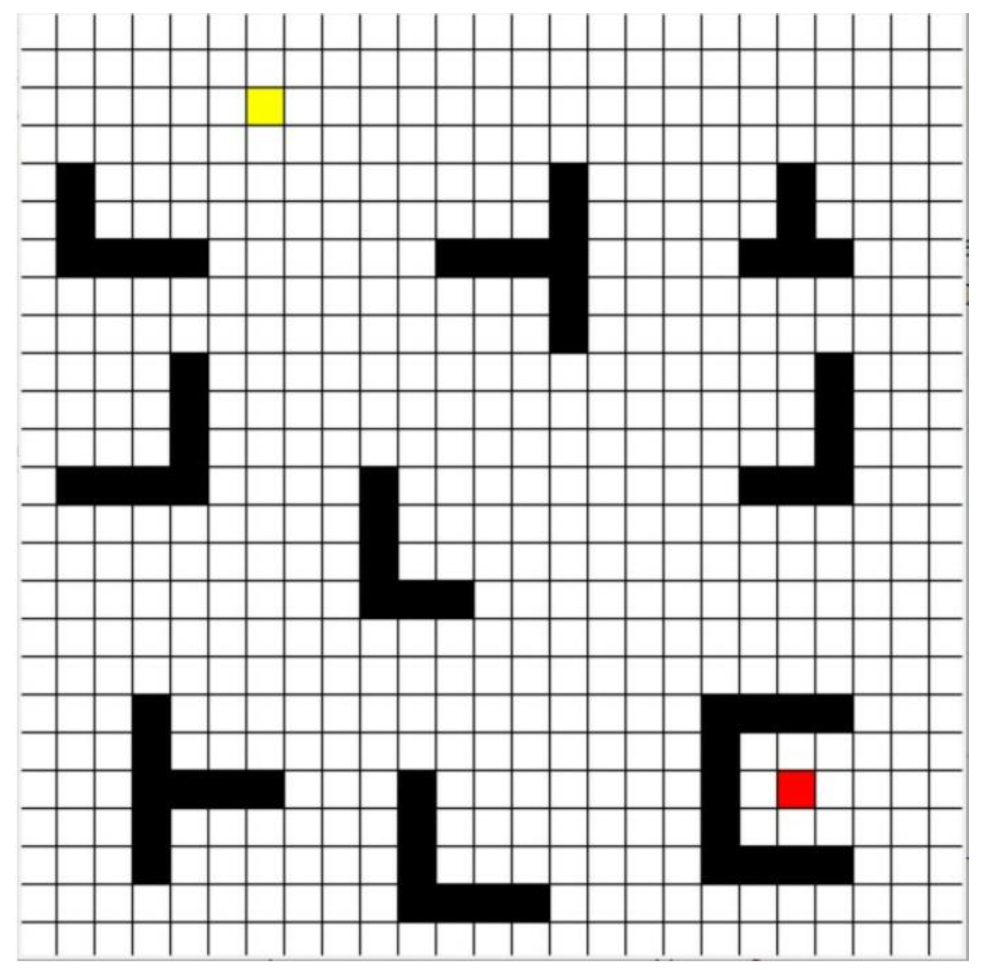The representation of the raster graph is shown in Figure 1.

In the figure, the yellow grid is the starting point of UGV, the red grid is the target point of UGV, and the black grids are the obstacles in the industrial park, such as buildings and green belts. The obstacles in the industrial park are inflated, the black grids are represented in the grid map, and the white grids are the road that can be freely passed in the industrial park.

3.2. UGV Settings

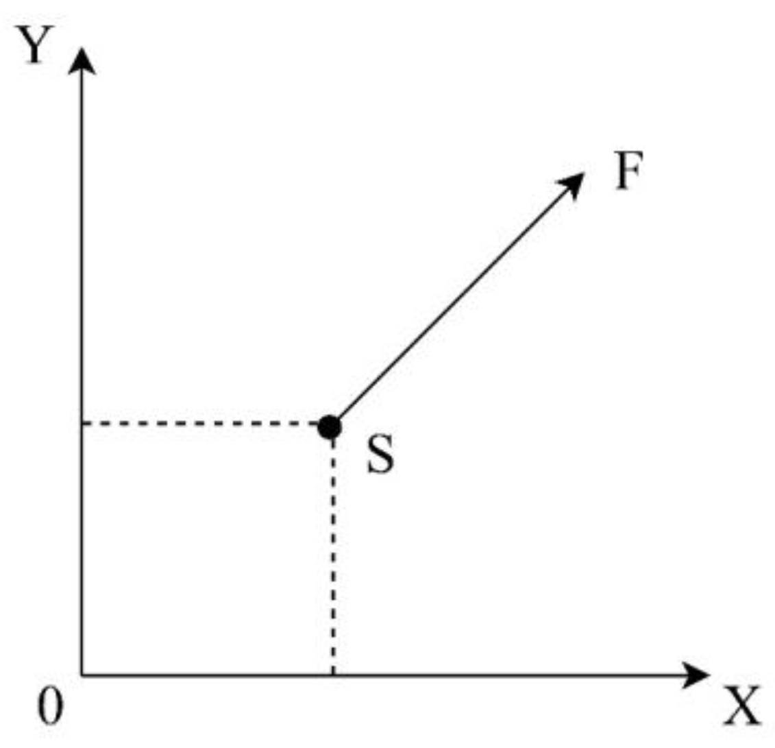
When planning the path of UGV, the motion state of UGV is the condition for the formation of an obstacle avoidance path. The geodetic coordinate system OXY is established, and the movement of UGV is shown in Figure 2. In addition, when planning the path of multiple UGVs, this paper assumes the following UGVs:

• Consider each UGV in motion as a particle;
• The movement speed and movement angle of each UGV are the same;
• The initial and target locations of each UGV are known;
• In each step, the UGV moves only once, that is, in the environment shown in Figure 1, the UGV can only move from one cell to another adjacent cell at a time;
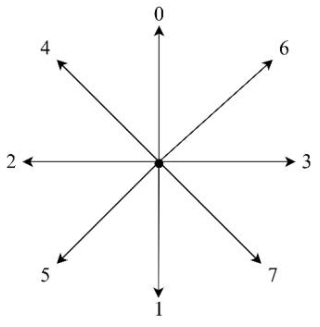
• Each UGV has eight directions of movement: up, down, left, right, upper left, lower left, upper right, and lower right, as shown in Figure 3.

In Figure 2, S is the starting point of UGV, and F is the target point of UGV. In each step, UGV selects one of the actions shown in Figure 3 to execute.

3.3. Multi-UGV Collision Avoidance Cooperation Mechanism

In the path planning problem for multiple UGVs, each UGV must avoid collisions with other UGVs in the process of finding the path. In the experiment of this paper, the initial position of each UGV is initially generated, only the initial position of each UGV is considered not overlapping, and then a multi-intelligent motion cooperation method is proposed to prevent UGV from colliding with other UGVs in the process of movement, and the final goal is that multiple UGVs can quickly find the target point in the same one, and the path generated by each UGV reaches the shortest.

We assume that three UGVs start from the starting point at the same time and move towards the target point at the same speed, and each UGV first observes whether it can move. If it cannot be moved, wait at the origin until it can be moved; if it can be moved, check whether it has encountered an obstacle, such as UGV1:UGV1, which determines whether it has encountered a fixed obstacle (that is, whether it has moved to the black area of the environment), and if it encounters an obstacle, it selects the action with the maximum Q value according to the improved $\epsilon -greedy$ strategy to execute; if UGV1 does not encounter a fixed obstacle during this movement, it is determined whether the current state of UGV2, UGV3 and UGV1 is collusion-free: if there is no collision, UGV1 will select the action with the maximum Q value according to the improved $\epsilon -greedy$ strategy to execute, if the state among the three is any of the upward collision, downward collision, left collision, right collision, upper left collision, lower left collision, upper right collision, lower right collision, at this time, if UGV1 waits in place for more than 1 s, continue to judge the relationship among the three UGV states, and select the action execution according to the relationship among the three, otherwise, wait in place until the waiting time is greater than 1 s. The specific cooperation mechanism is shown in Figure 4, and the same cooperation mechanism is followed in the process of each UGV movement.

3.4. Evaluation Indexes

The performance of the algorithm proposed in this paper is mainly evaluated from the average shortest path step, average path length, average calculation time, average reward, and simultaneous convergence of UGVs in one iteration and step convergence.

3.4.1. Average Shortest Path Steps

$$S={\displaystyle \sum _{u=1}^l{\displaystyle \sum _{i=1}^n{s}_{1i}}}/\left(n\times l\right)$$

(1)

where $i$ is the number of UGVs, $n$ is the number of UGVs, $s_{1i}$ is the shortest number of path steps for each UGV in path planning.

3.4.2. Average Path Length

In this paper, the path length generated by each UGV is calculated using the Euclidean distance, the path length of each UGV is as follows:

$$d_i=\sqrt{{\displaystyle \sum _{p=1}^m{\left(x_p-y_p\right)}^2}}$$

(2)

where $d_i$ is the path length of the first $i$ UGV, $p$ is the number of steps in the process of generating the final path of the UGV, $\left(x_p,y_p\right)$ is the position coordinate of the UGV when it moves for the $p$.

$$d={\displaystyle \sum _{u=1}^l{\displaystyle \sum _{i=1}^n{d}_i}}/\left(n\times l\right)$$

(3)

where $d$ is the average path length and $i$ is the number of UGVs.

3.4.3. Average Calculation Time

$$t={\displaystyle \sum _{u=1}^l{t}_i}/l$$

(4)

where $t$ is the average calculation time, $t_i$ is the calculation time of the $i$ UGV.

3.4.4. Average Rewards

$$r={\displaystyle \sum _{u=1}^l{\displaystyle \sum _{i=1}^n{r}_i}/\left(n\times l\right)}$$

(5)

where $r$ is the average reward and $r_i$ is the reward function value of the $i$ UGV.

The simultaneous convergence of UGVs in one iteration and the convergence of the reward function are compared and analyzed in the images of Section 5.3.1 and Section 5.3.2.

3.5. Objective Function

In the process of multi-UGV path planning, different factors affecting the effect of multi-UGV path planning are considered, including the shortest path steps in the training process of UGV, the length of the planned path, the time used for planning, the reward of UGV, and the convergence of the algorithm. The objective function also evaluates these factors at design time, so in this study, the objective function of multi-UGV path programming is summarized as Equation (6):

$$f=f_S+f_d+f_r+f_c$$

(6)

where $f_S$ is the smallest average shortest path step of UGVs, $f_d$ is the shortest average path length of UGVs, $f_r$ is the shortest average calculation time of OWS Q-learning algorithm under the same experimental environment setting, the average reward function value of UGVs is the largest, $f_c$ is UGVs to achieve the target point in a round of iterative learning, $f$ is a combination of the above four indexes.

4. OWS Q-Learning Algorithm

Reinforcement learning, as a learning method of machine learning, is an artificial intelligence algorithm that does not require prior knowledge and acts based on feedback from the environment. Through continuous interaction with the environment, trial, and error, the specific purpose is finally achieved, or the overall action benefit is maximized. It does not need the label of the training data, but it needs to know whether the feedback given by the environment for each step is a reward or a punishment. The feedback can be quantified, and the behavior of the training object is constantly adjusted based on the feedback. Reinforcement learning is mainly composed of five parts: agent, environment, state, action, and reward.

Agent: The subject of reinforcement learning training.

Environment: The environment in which the agent is located.

State (S): The state in which the current environment and agent are located, because the position of the agent is constantly changing, the entire state is changing, and the state contains the state of the agent and environment.

Action (A): An action set that the agent can take based on the current state.

Reward (R): The agent takes a specific action under the current state and obtains certain feedback from the environment as a reward.

State transition is represented by the $p$ function:

$$p(s^{\prime }|s,a)=p(S^{\prime }=s^{\prime }|S=s,A=a)$$

(7)

This is a conditional probability density function that represents the probability of the $p$ function output if the current state $s$ and the action $a$ are observed. The framework of reinforcement learning is shown in Figure 5:

$S_t$ is the state of the environment at $t$ moment, $A_t$ is the action that the agent performs at $t$ moment in the environment, $A_t$ makes the state of the environment change to $S_{t+1}$. In the new state, the environment generates a new feedback $R_{t+1}$, and the agent performs a new action $A_{t+1}$ according to $S_{t+1}$ and $R_{t+1}$, and so on until the end of the iteration.

In reinforcement learning, agents learn to solve sequential decision problems, which are usually described by the Markov decision process (MDP). It is used to describe and solve the problem hypothesis that agents learn strategies to maximize returns or achieve specific goals in the process of interacting with the environment. The quaternion of the Markov decision process (MDP) is $<S,A,R,P>$, where $S$ is the set of states, $A$ is the set of actions, $R$ is the reward function, $R_t=R\left(S_t,A_t\right)$ is the reward obtained by the agent after executing $A_t$ under state $S_t$, $P$ is the state transition probability, denoted as $P\left(S_{t+1},R_t|S_t,A_t\right)$. It indicates the probability distribution of $t$ moment state $S_t$, after executing action $A_t$, obtaining a reward $R_t$ and the next state is $S_{t+1}$.The complete Markov decision model is shown in Figure 6.

In MDP, the status $S_{t+1}$ and reward $R_{t+1}$ depend only on the previous state $S_t$ and action $A_t$, as described by the following function:

$$p\left(s^{\prime },r|s,a\right)=Pr\left\{R_{t+1}=r,S_{t+1}=s^{\prime }|S_t,A_t\right\}$$

(8)

In the process of learning, the agent tries to maximize the cumulative return, and the estimated discounted return $\gamma$ expressed by the discount rate $G_t$ is:

$$G_t=\underset{k=0}{\stackrel{\infty }{\Sigma }}{\gamma }^k{R}_{t+k+1}, 0\le \gamma \le 1$$

(9)

The agent follows the policy $\pi \left(a|s\right)$, which is a function of the probability of selecting each possible action from that state. It represents the probability that the agent chooses to perform action $A_t=a$ in the case of $S_t=s$. The status value function ${\nu }_{\pi }\left(s\right)$ is the expected discounted return when the agent follows the strategy $\pi$, which can be expressed by the formula:

$${\nu }_{\pi }\left(s\right)={\mathbb{E}}_{\pi }\left[G_t|S_t=s\right]$$

(10)

Similarly, the state–action value function $Q_{\pi }\left(s,a\right)$ is defined as the expected return value that starts at state $s$ and takes action $a$. The state–action value function $Q_{\pi }\left(s,a\right)$ is expressed by the formula as:

$$Q_{\pi }\left(s,a\right)={\mathbb{E}}_{\pi }\left[G_t|S_t=s,A_t=a\right]$$

(11)

The optimal state–action value function is defined as $Q_{*}$, expressed by the formula:

$$Q_{*}\left(s,a\right)=\underset{\pi }{max}{Q}_{*}\left(s,a\right)$$

(12)

The optimal Bellman equation for the state–action value function is:

$$Q_{*}\left(s,a\right)=\mathbb{E}[R_{t+1}+\underset{a^{\prime }}{\gamma max{Q}_{*}}(S_{t+1},a^{\prime })|S_t=s,A_t=a]$$

(13)

Reinforcement learning algorithms use these optimality equations to iterate to update the strategy followed by the agent.

Based on the above, the idea chain of reinforcement learning solution is: solution of reinforcement learning→solution of optimal strategy→solution of optimal value function→solution of Bellman equation, that is, the solution problem of reinforcement learning finally boils down to solving the optimal Bellman equation [53].

4.1. Q-Learning Algorithm

The Q-learning algorithm was first proposed by Watkins et al. in 1989 as a method for solving reinforcement learning tasks [54], using a state–action value function $Q\left(s,a\right)$. The general idea of the algorithm is that the agent keeps trying in an unknown environment. In the process of trying, the agent constantly adjusts the strategy based on the feedback obtained, and finally generates a better strategy. The update process of the Q-learning algorithm’s value function $Q\left(s,a\right)$ is as follows:

$$Q\left(s,a\right)\leftarrow Q\left(s,a\right)+\alpha \left[R+\gamma \underset{a^{\prime }}{max}Q\left(s^{\prime },a^{\prime }\right)-Q\left(s,a\right)\right]$$

(14)

where $Q\left(s,a\right)$ indicates that the agent’s state at $t$ moment is $s_t$, the sum of the optimal reward discount obtained after executing the action $a_t$. $\alpha$ is the learning rate, which represents the impact of the current training sample on the current learning. $\gamma$ is the discount factor [55], which reflects the proportion of the value of future rewards at the current moment.

The updates of the value function $Q\left(s,a\right)$ in the Q-learning algorithm are as follows: under the state $S$, the agent uses the $\epsilon -greedy$ strategy to select the action $a$, executes the action $a$, obtains the immediate reward $r$, and the agent transfers to the next state $S^{\prime }$, at which time the agent selects the $a$ that makes the largest $Q(s^{\prime },a)$ as the next action $a^{\prime }$ to update the value function (12). $a^{\prime }$ only participates in the update of the value function and does not really execute. The action performed in the next state $S^{\prime }$ is re-selected using the $\epsilon -greedy$ strategy after the value function is updated. The agent from the beginning to the endpoint is called an episode. The pseudocode for the Q-learning Algorithm 1 is as follows:

Algorithm 1 Q-learning algorithm

Input: state set $S$, action set $A$, reward function $R$

Output: $\mathrm{optimal} \mathrm{state}–\mathrm{action} \mathrm{value} \mathrm{function} Q_{*}\left(s,a\right)$, $\mathrm{from} \mathrm{the} \mathrm{optimal} \mathrm{state}–\mathrm{action} \mathrm{value} \mathrm{function} \mathrm{to} \mathrm{obtain} \mathrm{the} \mathrm{optimal} \mathrm{strategy} {\pi }_{*}\left(S\right)$

Process:

1. Initialize the Q table and have a Q value of 0 for all state–action pairs

2. $\pi$: derived from Q

3. If strategy $\pi$ is not optimal

4. $\mathrm{For} \mathrm{all} \mathrm{states} s\in S,a\in A$

5. $\mathrm{Update} \mathrm{the} \mathrm{state}–\mathrm{action} \mathrm{value} \mathrm{function} Q\left(s,a\right)$:         $Q\left(s,a\right)\leftarrow Q\left(s,a\right)+\alpha \left[R+\gamma \underset{a^{\prime }}{max}Q\left(s^{\prime },a^{\prime }\right)-Q\left(s,a\right)\right]$

6. If the strategy is optimal at this point, end the calculation, otherwise skip back to step four

4.2. Speedy Q-Leaning Algorithm

Although the Q-learning algorithm is a classical algorithm of reinforcement learning, the algorithm has certain limitations [56]. When the number of state actions of the agent is limited, the Q-learning algorithm can converge to the optimal strategy, but when the discount factor $\gamma$ is close to 1, the convergence speed of the Q-learning algorithm will become very slow [56]. The speedy Q-learning algorithm was first proposed in 2011 by Azar et al. [57]. The speedy Q-learning algorithm improves the Q-learning algorithm by using an aggressive learning rate, replacing the learning rate of an updated criterion in the Q-learning algorithm with a larger learning rate, which improves the convergence speed of the algorithm [57]. In essence, the speedy Q-learning algorithm replaces the estimation function of the historical Q value with that of the current Q value and selects a more efficient estimator, thus improving the convergence speed of the Q-learning algorithm [53].

Assuming that $M\left(s^{\prime },a^{\prime }\right)=\underset{a^{\prime }}{max}Q\left(s^{\prime },a^{\prime }\right)$, $M_{-}\left(s^{\prime },a^{\prime }\right)$ represents the maximum value function value of the next state when the Q value of state action $\left(s,a\right)$ is updated in the previous iteration step. The Q value update process of the speedy Q-learning algorithm [53] is:

$$Q\left(s,a\right)=\left(1-\alpha \right)Q\left(s,a\right)+\alpha \left[r+\gamma M_{-}\left(s^{\prime },a^{\prime }\right)\right]+\left(1-\alpha \right)\gamma \left[M\left(s^{\prime },a^{\prime }\right)-M_{-}\left(s^{\prime },a^{\prime }\right)\right]$$

(15)

The pseudocode for the speedy Q-learning Algorithm 2 is as follows:

Algorithm 2 Speedy Q-learning algorithm

Input: state set $S$, action set $A$, reward function $R$

Output:$\mathrm{optimal} \mathrm{state}–\mathrm{action} \mathrm{value} \mathrm{function} Q_{*}\left(s,a\right)$, $\mathrm{from} \mathrm{the} \mathrm{optimal} \mathrm{state}–\mathrm{action} \mathrm{value} \mathrm{function} \mathrm{to} \mathrm{obtain} \mathrm{the} \mathrm{optimal} \mathrm{strategy} {\pi }_{*}\left(S\right)$

Process:

1. $\mathrm{Initialize} Q\left(s,a\right)=M\left(s,a\right),s$, and have a Q value of 0 for all state–action pairs

$\mathrm{for} i=1$ to episodes

2. Repeat:

3. $\mathrm{Based} \mathrm{on} \mathrm{the} \mathrm{value} \mathrm{function} \mathrm{Q}, \mathrm{use} \mathrm{a} \mathrm{strategy} (\mathrm{such} \mathrm{as} \mathrm{strategy} \epsilon -greedy)$ to select action $a$ in state $s$;

4. Execute action $\mathrm{a}$ to obtain instant reward $r$$\mathrm{and} \mathrm{obtain} \mathrm{the} \mathrm{next} \mathrm{state} s^{\prime }$;

5. $a^{*}\leftarrow argmaxQ(s^{\prime },a^{\prime })$

6. $\sigma \leftarrow \left(2\alpha -1\right)\gamma M\left(s,a\right)$

7. $M\left(s,a\right)\leftarrow Q\left(s^{\prime },a^{*}\right)$

8. $Q\left(s,a\right)\leftarrow \left(1-\alpha \right)\left[Q\left(s,a\right)+\gamma M\left(s,a\right)+\alpha r+\sigma \right]$

9. $s\leftarrow s^{\prime }$

Until $s$ is terminated

End for

4.3. OWS Q-Learning Algorithm

In this paper, Q-learning algorithm has been improved in three aspects, namely, Q function update mode, learning rate and $\epsilon -greedy$ strategy.

4.3.1. Q Function Updating

In a random environment, the performance of the reinforcement learning algorithm Q-learning is poor [58]. The use of the maximum action value as an approximation of the maximum expected action value in the Q-learning algorithm introduces a positive bias, resulting in overestimation and affecting the overall performance of the algorithm [58]. The speedy Q-learning algorithm essentially takes the estimation function of the current Q value as an estimate of the historical Q value. Although the convergence speed of the algorithm is improved, it has the same overestimation problem as the Q-learning algorithm, resulting in a poor strategy for the agent to update the Q value in the early stage of training. Using the estimation function of the current Q value as the estimation function of the historical Q value will produce a large error, which makes the convergence speed of the algorithm slower at the beginning of the iteration [59].

Aiming at the problem of the slow convergence speed of the Q-learning algorithm, and in order to further improve the convergence speed of the speedy Q-learning algorithm, this paper proposes the OWS Q-learning algorithm. This algorithm changes the way the Q function is updated and obtains a new estimation strategy by assigning different weights to the maximum estimate of the next state Q value and the maximum estimate of the current state Q value in the historical Q table, so as to obtain a more accurate estimate. Where the value of weight $\beta$ is defined as:

$$\beta =\frac{\left|\underset{a^{\prime }}{max}Q\left(s^{\prime },a^{\prime }\right)-\underset{a^{\prime }}{min}Q\left(s^{\prime },a^{\prime }\right)\right|}{c+\left|\underset{a^{\prime }}{maxQ}\left(s^{\prime },a^{\prime }\right)-\underset{a^{\prime }}{min}Q\left(s^{\prime },a^{\prime }\right)\right|}$$

(16)

where $\beta \in \left(0,1\right)$ and $c$ is a free parameter that can be adjusted according to the environment of the experiment.

Suppose that $M\left(s^{\prime },a^{\prime }\right)=\underset{a^{\prime }}{max}Q\left(s^{\prime },a^{\prime }\right)$, $M_{-}\left(s^{\prime },a^{\prime }\right)$ represent the value function Q value of the previous iteration step update state action Q value when the next state is valued, and the Q function of the algorithm is updated as follows:

$$\begin{gathered} Q\left(s,a\right)\leftarrow \alpha \left\{r+\gamma \left[\beta M\left(s^{\prime },a^{\prime }\right)+\left(1-\beta \right)M_{-}\left(s^{\prime },a^{\prime }\right)\right]-Q\left(s,a\right)\right\} \\ +\left(1-\alpha \right)\gamma \left[M\left(s^{\prime },a^{\prime }\right)-M_{-}\left(s^{\prime },a^{\prime }\right)\right] \end{gathered}$$

(17)

The above is an improvement in the update method of the Q function, and an optimization and improvement in the learning rate $\alpha$ and $\epsilon -greedy$ strategies.

4.3.2. Optimize Learning Rate

The learning rate $\alpha$ controls the learning progress of the model in the process of iteration and determines the degree to which the newly obtained information overwrites the original information [60]. $\alpha =0$ means that the agent cannot do anything to learn and only uses prior knowledge, and $\alpha =1$ means that the agent only considers the latest information and ignores prior knowledge [60]. The speed and accuracy of the convergence of the Q-learning algorithm are seriously affected by the learning rate, if the value of the learning rate is too large, the learning will accelerate, but the noise in the environment will also be absorbed, so the Q value will fluctuate greatly, and it is difficult to converge [59]. On the contrary, if the value of the learning rate is too small, then the Q value will converge slower, making it difficult for the training of the agent to keep up with changes in the environment [59]. In most Q-learning applications, the learning rate is usually set as a constant, usually $\alpha$ takes a value between 0.01–0.1, and a constant learning rate is often used, such as taking $\alpha =0.1$ in experiments, so it cannot meet the needs of dynamic and fast learning.

If the learning rate is fixed in practice, when the algorithm reaches convergence, the Q value will swing in a large area near the optimal value. However, when the learning rate decreases with the increase in the number of iterations, the algorithm will converge, and the Q value will swing in a smaller area near the optimal value. In this paper, the learning rate $\alpha$ is optimized, so that $\alpha$ decayed along with the number of training rounds. In the early stage of training, the learning rate $\alpha$ is larger, the new information covers the original information less, and the agent considers less prior knowledge, with the increase in training rounds, the learning rate gradually decreases, the new information covers the old information more, the agent considers more prior knowledge, ${\alpha }_1$ is used to represent the improved learning rate. The optimization result of the learning rate is as follows:

$${\alpha }_1=\frac{1}{k+10}$$

(18)

where $k$ is the number of training rounds episodes, $k=0,1,\dots \left(k\in Z\right)$, ${\alpha }_1$ with the dynamic change in the number of training rounds of the agent, the value of $k$ is small when the agent first starts training, in order to ensure that the value of ${\alpha }_1$ is meaningful, the denominator part is set to $k+10$ after multiple experimental comparisons.

4.3.3. Improve ε—Greedy Strategy

The entire learning process of reinforcement learning can be divided into two stages: (1) exploration stage: the agent randomly explores the environment to learn the current environment; (2) utilization stage: the agent uses the environmental information that has been explored to achieve the goal. The balance of exploration and utilization is also a key challenge in reinforcement learning, commonly used in a heuristic exploration algorithm $\epsilon -greedy$. The algorithm selects the action with the largest Q value from the action set $\mathrm{A}$ with a certain probability, randomly selects the action with the probability of $\epsilon$, and selects the action with the largest Q value with a probability of $1-\epsilon$. The mathematical expression for the $\epsilon -greedy$ strategy is:

$${\pi }^{\epsilon }\left(a\right)=\left\{\begin{array}{l}\underset{a\in A}{\mathrm{argmax}}Q\left(a\right), \mathrm{take} \mathrm{probability} 1-\epsilon \\ \mathrm{randomly} \mathrm{select} \mathrm{action} \mathrm{A}, \mathrm{take} \mathrm{probability} \epsilon \end{array}\right\}$$

(19)

where $a$ is a randomly generated real number between (0, 1).

Strategy $\epsilon -greedy$ can update and adjust the strategy in time according to the selected action and the instant reward obtained, so as to avoid the algorithm falling into a suboptimal state. Parameter $\epsilon$ is difficult to set accurately. When $\epsilon$ is large, the algorithm has strong flexibility, a fast exploration rate, and can quickly explore potential high rewards, so the convergence speed of the algorithm is faster and the adaptability to environmental changes is strong, but the overall cumulative reward may be very low. When $\epsilon$ is small, the algorithm has strong stability, the exploration rate is slower, and there is more probability of making good use of the better reward that have been explored, but it will make the convergence speed of the algorithm slower, and will make the algorithm less adaptable to environmental changes, but it is possible to obtain a higher cumulative reward in the end.

This paper optimizes and improves the value of $\epsilon$, and sets the value of $\epsilon$ to the form of segments. In order to balance the relationship between exploration and utilization in reinforcement learning, to ensure that the agent can fully explore in the early stage of training, and as the training progresses, the agent can make full use of the information explored for more effective learning, and the initial value of $\epsilon$ is set to 0.85 under multiple experiments, as shown in Equation (20):

$$\epsilon =\{\begin{array}{c}0.85+episode\ast 0.0001, episode\le m\\ 1, else\end{array}$$

(20)

where $m$ is a positive integer less than the maximum number of rounds, set according to the experimental environment.

The pseudocode for the OWS Q-learning Algorithm 3 is as follows:

Algorithm 3 OWS Q-learning algorithm

Input:  state set $S$, action set $A$, reward function $R$

Output:$\mathrm{optimal} \mathrm{state}–\mathrm{action} \mathrm{value} \mathrm{function} Q_{*}\left(s,a\right)$, $\mathrm{from} \mathrm{the} \mathrm{optimal} \mathrm{state}–\mathrm{action} \mathrm{value} \mathrm{function} \mathrm{to} \mathrm{obtain} \mathrm{the} \mathrm{optimal} \mathrm{strategy} {\pi }_{*}\left(S\right)$

Process:

1. $\mathrm{Initialize} Q\left(s,a\right)=M\left(s,a\right),s$, and have a Q value of 0 for all state–action pairs

$\mathrm{for} \mathrm{i}=1 \mathrm{to} \mathrm{episodes}$

2. Repeat:

3. Based on the value function Q, the improved $\epsilon -greedy$ strategy is used to select action $a$ under state $s$;

4. Execute action $a$, obtain instant reward $r$$, \mathrm{obtain} \mathrm{the} \mathrm{next} \mathrm{state} s^{\prime }$;

5.  $a^{*}\leftarrow arg\underset{a^{\prime }}{max}Q\left(s^{\prime },a^{\prime }\right)$

6. $\sigma \leftarrow M\left(s,a\right)$

7. $M\left(s,a\right)\leftarrow Q\left(s^{\prime },a^{*}\right)$

8. $Q\left(s,a\right)\leftarrow \alpha \left\{r+\gamma \left[\beta M\left(s,a\right)+\left(1-\beta \right)\sigma \right]-Q\left(s,a\right)\right\}+\left(1-\alpha \right)\gamma \left[M\left(s,a\right)-\sigma \right]$

9. $s\leftarrow s^{\prime }$

Until $s$ is terminated

End for

4.3.4. Reward Function

In reinforcement learning, the reward function is an important factor affecting the result of the path planning. The ultimate goal of reinforcement learning is to maximize the cumulative return expectation from the initial state to the target state, and the reward function defines the value that the agent can obtain by performing different actions under the current environment. Based on the UGV environment, the reward function in this paper is set as follows:

$$R=\left\{\begin{array}{l}{r}_1,\mathrm{the} \mathrm{UGV} \mathrm{reaches} \mathrm{the} \mathrm{target} \mathrm{point} \\ r_2, \mathrm{the} \mathrm{UGV} \mathrm{hit} \mathrm{an} \mathrm{obstacle} \\ r_3, \mathrm{the} \mathrm{UGV} \mathrm{movement} \mathrm{to} \mathrm{environmental} \mathrm{boundaries}\\ r_4, \mathrm{else}\end{array}\right\}$$

(21)

In Equation (21), the value of $r_1,r_2,r_3 \mathrm{and} r_4$ need to be set according to the experimental environment in which the UGV is located.

5. Simulation Experiments and Analysis

The time series difference method is a model-free reinforcement learning algorithm, which can be divided into two types: online control algorithm SARSA and offline control algorithm Q-learning [61]. Among them, the SARSA algorithm was first mentioned by Rummery et al. [62] in 1994. The biggest difference between the SARSA algorithm and the Q-learning algorithm is the update method of the Q function, the Q-learning algorithm is bolder in the choice of actions, while the SARSA algorithm is more conservative in the selection of actions [61].

In order to verify the effectiveness of the proposed algorithm, in the simulation experiment in this section, the Q-learning algorithm, SARSA algorithm, speedy Q-learning algorithm, and the proposed OWS Q-learning algorithm are used to plan the paths of three UGVs in the industrial park, and the experimental results are compared and analyzed. The configuration of the experimental system is Intel(R) Core(TM) i5-6200U CPU @ 2.30 GHz 2.40 GHz, and the simulation experiments are conducted in the Python3 package.

5.1. Parameter Settings

In order to compare the algorithms, the Q-learning algorithm, SARSA algorithm, speedy Q-learning algorithm, and the OWS Q-learning algorithm proposed in this paper are unified experimental parameter settings as shown in

Table 1. Experimental parameter settings.

Parameter	Numeric Value
Learning rate α	0.02
Learning rate α1	1/(k + 10)
Explore factors ε	0.9
Discount factor γ	0.9
Reward function r1	120
Reward function r2	−120
Reward function r3	−100
Reward function r4	−3
m	400
n	3
l	10
Max episode	1800

.

5.2. Path Planning Scenarios

The complexity of the experimental scenario is mainly defined by the shape, proportion, and density of obstacles in the scenario, and the scenario is divided into simple scenarios and complex scenarios. The number of obstacles in simple scenarios is small and the shape of obstacles is regular. The number of obstacles in complex scenarios is large or the shape of obstacles is irregular. In order to verify the completeness and robustness of the proposed algorithm, this paper sets up three different experimental scenarios according to the division of the complexity of the experimental scenario, and the scenarios are complicated in turn. In order to verify the collision-free nature of the path planned by the proposed algorithm for multiple UGVs, the settings of the start point and target point of UGV1 and UGV3 do not show the relationship of upper and lower correspondence but set the relationship of cross-correspondence.

5.2.1. Simulation Scenarios That Contain Only Convex Obstacles

The structure of the scenario uses the Tkinter module in Python, and the position of each agent is represented by the position coordinates of the two points of the upper left corner and the lower right corner of the square, and the side length of a grid is set to 20. The simple scenario is equipped with eight regular-shaped obstacles, 38 × 38 environment size. The top yellow square, blue square, and red square in the environment diagram represent UGV1, UGV2, and UGV3, respectively, and the square at the bottom of the environment map is the target point of the UGV corresponding to the color. The coordinates of the start point and target point of each UGV are shown in

Table 2. The starting and target points of the UGV obstacle avoidance path.

Number	The Coordinates of the Starting Point	The Coordinates of the Target Point
1	(120, 40, 140, 60)	(120, 680, 140, 700)
2	(360, 40, 380, 60)	(360, 680, 380, 700)
3	(620, 40, 640, 60)	(620, 680, 640, 700)

.

In the simple scenario, the path planning simulation results of the SARSA algorithm, Q-learning algorithm, speedy Q-learning algorithm, and the OWS Q-learning algorithm are shown in Figure 7.

From the path planning results in the simple scenario, the SARSA algorithm plans the route from the starting point to the target point for UGV2 and UGV3, and the route is tortuous. The Q-learning algorithm mapped out a route from the start point to the target point for the three UGVs, but the route was complicated. Compared with the Q-learning algorithm, the SARSA algorithm is more conservative in action selection, so under the same training and learning round, the SARSA algorithm does not complete the task of planning the path for all three UGVs. The speedy Q-learning algorithm and the proposed OWS Q-learning algorithm both plan the route from the starting point to the target point for the three UGVs. The specific experimental results are shown in

Table 3. Comparison of simulation results of the four algorithms containing only convex obstacles.

Index	Number	SARSA	Q-Learning	Speedy Q-Learning	OWS Q-Learning
Shortest path steps	UGV1	0	261	37	35
	UGV2	106	178	34	34
	UGV3	556	212	36	34
Path length (unit)	UGV1	0	279.98	46.36	45.60
	UGV2	114.47	181.41	41.70	43.18
	UGV3	574.04	231.04	46.60	42.94
Calculation time (s)	—	10,191	8545	5007	3345

.

The experimental results in Table 3 show that the calculation time of the OWS Q-learning algorithm is the shortest in the same experimental scenario. In general, compared with the other three comparison algorithms, the OWS Q-learning algorithm has the shortest calculation time, the most complete planned path, and the shortest planned path compared with the other three comparison algorithms.

5.2.2. Simulation Scenarios That Contain Only Non-Convex Obstacles

In order to verify the robustness of the OWS Q-learning algorithm, the experimental scenario is complicated on the basis of the experimental scenario setting in Section 5.2.1. The more complex scenario is equipped with eight irregularly shaped obstacles, and the environment size is still 38 × 38. The coordinates of the start and target points of each UGV are shown in Table 2.

In the complex scenario, the path planning simulation results of the SARSA algorithm, Q-learning algorithm, speedy Q-learning algorithm, and the OWS Q-learning algorithm are shown in Figure 8.

The path planning results in the complex scenario show that the SARSA algorithm does not plan the path for UGV1, the Q-learning algorithm does not plan the path for UGV3, and the speedy Q-learning algorithm and the OWS Q-learning algorithm have planned collision-free paths for the three UGVs. Compared with the path planning results in the simple scenario, it shows that the SARSA algorithm and Q-learning algorithm cannot solve the multi-UGV path planning problem well. The specific experimental results are shown in

Table 4. Comparison of simulation results of four algorithms containing only non-convex obstacles.

Index	Number	SARSA	Q-Learning	Speedy Q-Learning	OWS Q-Learning
Shortest path steps	UGV1	0	285	41	32
	UGV2	178	166	35	35
	UGV3	195	0	38	37
Path length (unit)	UGV1	0	298.61	50.36	42.60
	UGV2	197.45	183.31	42.53	44.36
	UGV3	209.94	0	49.43	48.43
Calculation time (s)	—	12,143	11,255	5453	3577

.

The results in Table 4 in the complex experimental scenario show that compared with the other three algorithms, the OWS Q-learning algorithm has the shortest path, the shortest path steps, and the shortest calculation time for UGVs. In general, in the complex scenario, the OWS Q-learning algorithm still shows the efficiency of solving the multi-UGV path planning problem.

5.2.3. Simulation Scenarios That Contain More Odd-Shaped Obstacles

On the basis of the experimental scenario setting in Section 5.2.2, the experimental scenario is complicated again to verify the robustness of the OWS Q-learning algorithm. In the more complex scenario, 12 irregularly shaped obstacles were set, and the environment size was still 38 × 38. The coordinates of the start and target points of each UGV are shown in Table 2.

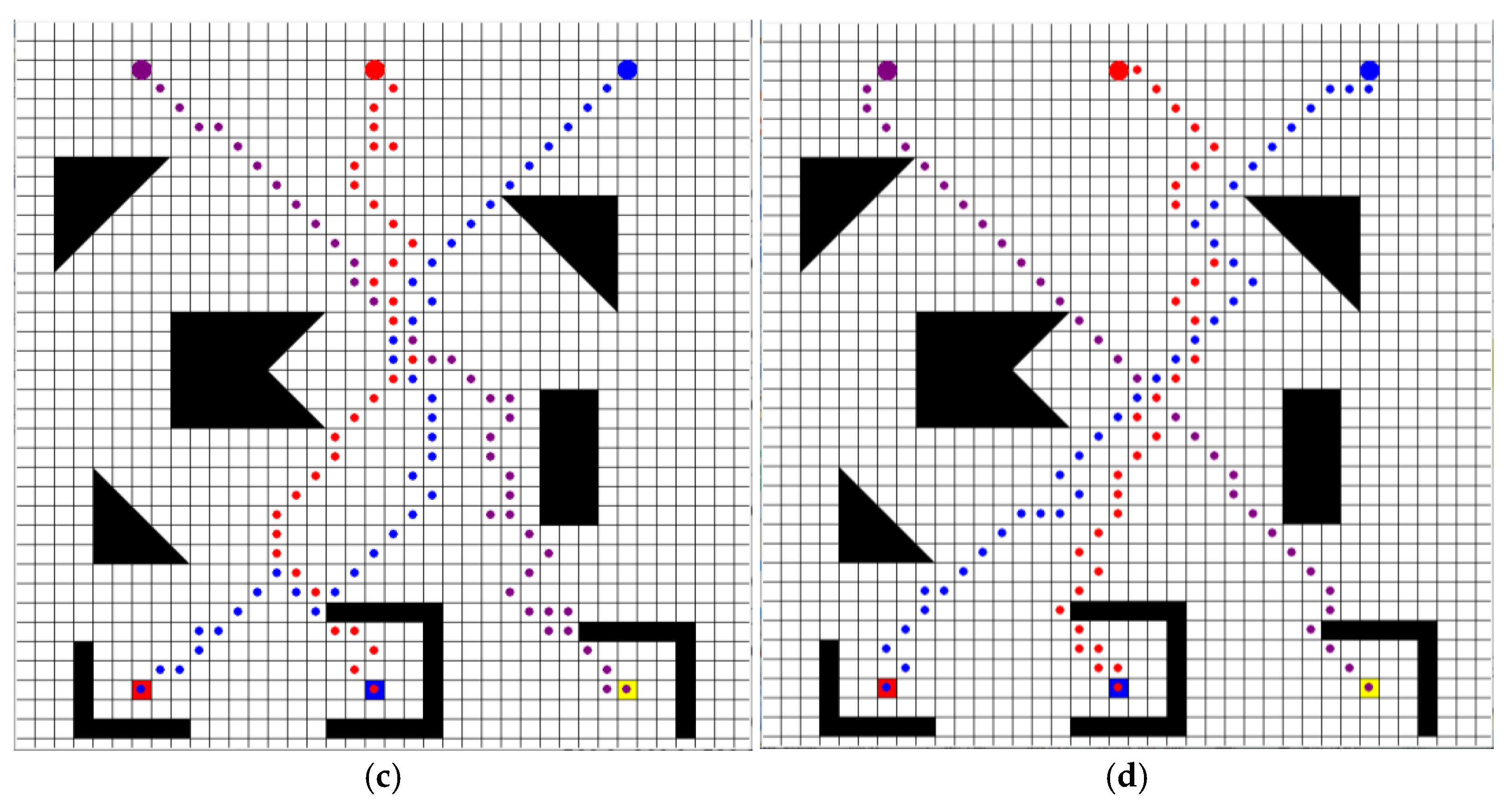
In the more complex scenario, the path planning simulation results of the SARSA algorithm, Q-learning algorithm, speedy Q-learning algorithm, and the OWS Q-learning algorithm are shown in Figure 9.

From the path planning results in the more complex scenario, the SARSA algorithm only plans the route from the starting point to the target point for UGV2. The Q-learning algorithm only maps out the route from the starting point to the target point for UGV2. Compared with the simulation results in the simple scenario and the complex scenario, we find that with the increase in complexity of the experimental scenario, the effectiveness of the SARSA algorithm and Q-learning algorithm in solving multi-UGV path planning problems is getting worse and worse. This is because the SARSA algorithm is conservative in action selection and the Q-learning algorithm converges slowly, so it is difficult for the SARSA algorithm and the Q-learning algorithm to achieve the goal of planning a path for each UGV under the same round of training. Only the speedy Q-learning algorithm and the OWS Q-learning algorithm mapped out the route from the start point to the target point for the three UGVs. The specific experimental results are shown in

Table 5. Comparison of simulation results of four algorithms containing more odd-shaped obstacles.

Index	Number	SARSA	Q-Learning	Speedy Q-Learning	OWS Q-Learning
Shortest path steps	UGV1	0	0	35	37
	UGV2	301	162	35	37
	UGV3	0	0	53	35
Path length (unit)	UGV1	0	0	45.60	48.01
	UGV2	319.53	174.89	44.77	45.53
	UGV3	0	0	61.77	45.18
Calculation time (s)	—	6789	9364	4149	3110

.

From the experimental results in Table 5, compared with the speedy Q-learning algorithm, the total path length planned by the OWS Q-learning algorithm for UGVs is shorter. Compared with the three comparison algorithms, the OWS Q-learning algorithm takes the shortest time under the same training episodes.

The simulation results in the above three experimental scenarios show that compared with the SARSA algorithm, Q-learning algorithm, and speedy Q-learning algorithm, under the same training episodes, the OWS Q-learning algorithm has the shortest calculation time and the shortest planned path length, and the best effect of solving the multi-UGV path planning problem, which verifies the stability and robustness of the OWS Q-learning algorithm.

5.3. Comparative Analysis of Algorithm Performance

5.3.1. Algorithm Convergence Analysis

Reinforcement learning is model-free learning, in the process of training, because the agent does not have any experience accumulation in the early stage of learning, it takes a lot of time to find the path, and the agent may encounter different obstacles in the process of searching. However, as learning progresses, the agent continues to accumulate experience and knowledge, so as the number of training rounds increases, the number of steps the agent needs in each round will also decrease.

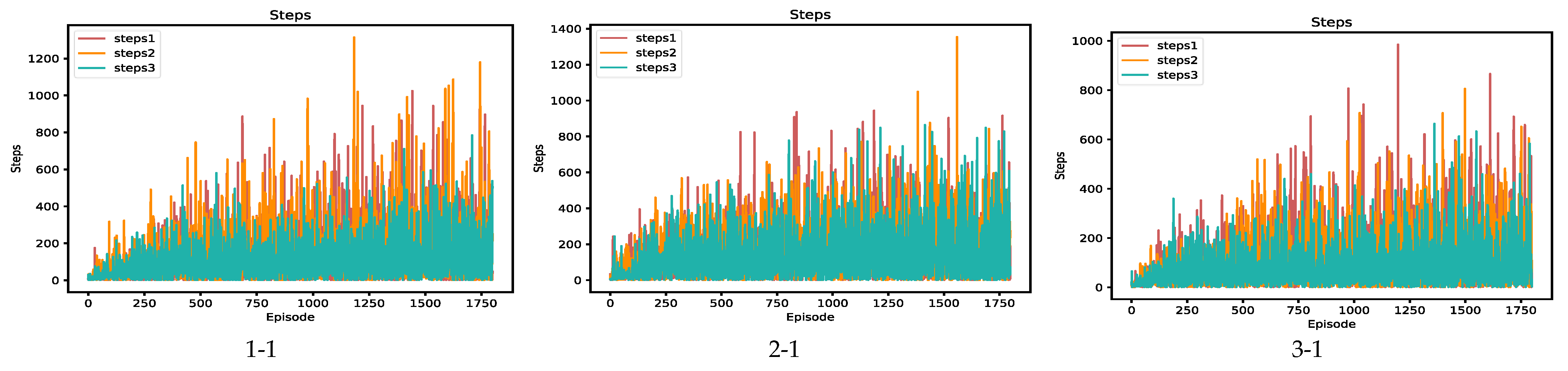
The changes in the number of steps in the training and learning process of the SARSA algorithm, Q-learning algorithm, speedy Q-learning algorithm, and OWS Q-learning algorithm in different scenarios are compared and analyzed. The steps of each UGV in the four algorithms in three scenarios are shown in Figure 10. The three different scenarios are recorded as scenarios 1, 2, and 3 in turn, among them, columns 1, 2, and 3 are the steps convergence result graphs of scenario1, scenario2, and scenario3, and rows 1, 2, 3, and 4 are the steps changes in UGV under SARSA algorithm, Q-learning algorithm, Speedy Q-learning algorithm, and OWS Q-learning algorithm.

Figure 10 results show that in the three experimental scenarios, the SARSA algorithm, Q-learning algorithm, and speedy Q-learning algorithm have no convergence trend under 1800 iterations of learning. In scenario1, after about 850 episodes of learning, the three UGVs in the OWS Q-learning algorithm can find their respective target points in the same round, and the training effect is relatively stable. In scenario2, after about 800 episodes of learning 3 UGVs in the OWS Q-learning algorithm, the 3 UGVs can find their respective target points in the same episode after that, and the results are relatively stable. In scenario3, after about 1000 episodes of learning 3 UGVs in the OWS Q-learning algorithm, the 3 UGVs can find their respective target points in the same episode after that, and the training effect is relatively stable. It can be seen that the OWS Q-learning algorithm proposed in this paper is effective for solving multiple UGV path planning problems.

5.3.2. UGVs Reward Analysis

The reward function changes in the three UGVs were compared and analyzed when the SARSA algorithm, Q-learning algorithm, speedy Q-learning algorithm, and OWS Q-learning algorithm were planned from the starting point to the target point. The reward changes in each UGV in the four algorithms in three scenarios are shown in Figure 11.

Among them, columns 1, 2, and 3 are the reward change result graphs of scenario1, scenario2, and scenario3. Rows 1, 2, 3, and 4 are the UGV changes under the SARSA algorithm, Q-learning algorithm, speedy Q-learning algorithm, and OWS Q-learning algorithm.

From the results of Figure 11, in the three experimental scenarios, the rewards of the 3 UGVs of the SARSA algorithm in 1800 iterative learning did not converge, and the reward function under each round fluctuated greatly, and the training effect of UGV in the process of finding the path was unstable. The reward of the 3 UGVs in the 1800 iterative learning of the Q-learning algorithm also did not converge, but compared with the SARSA algorithm, the fluctuation range of the reward function of the 3 UGVs was alleviated. Under the speedy Q-learning algorithm, the reward of 3 UGVs in 1800 learning iterations also did not converge but compared with the SARSA algorithm and Q-learning algorithm, the fluctuation range of each UGV reward function slowed down. In scenario1, the reward function converges to around 0 after about 850 iterations of learning for three UGVs in the OWS Q-learning algorithm. In scenario2, the reward function converges to around 0 after about 800 iterations of learning for 3 UGVs in the OWS Q-learning algorithm. In scenario3, the reward function converges to around 0 after about 1000 iterations of learning for 3 UGVs in the OWS Q-learning algorithm.

In general, compared with the changes in reward function under the SARSA algorithm, Q-learning algorithm, and speedy Q-learning algorithm, the OWS Q-learning algorithm proposed in this paper has a significant convergence trend of reward function in multi-UGV path planning problems.

5.3.3. Algorithm Performance Comparison

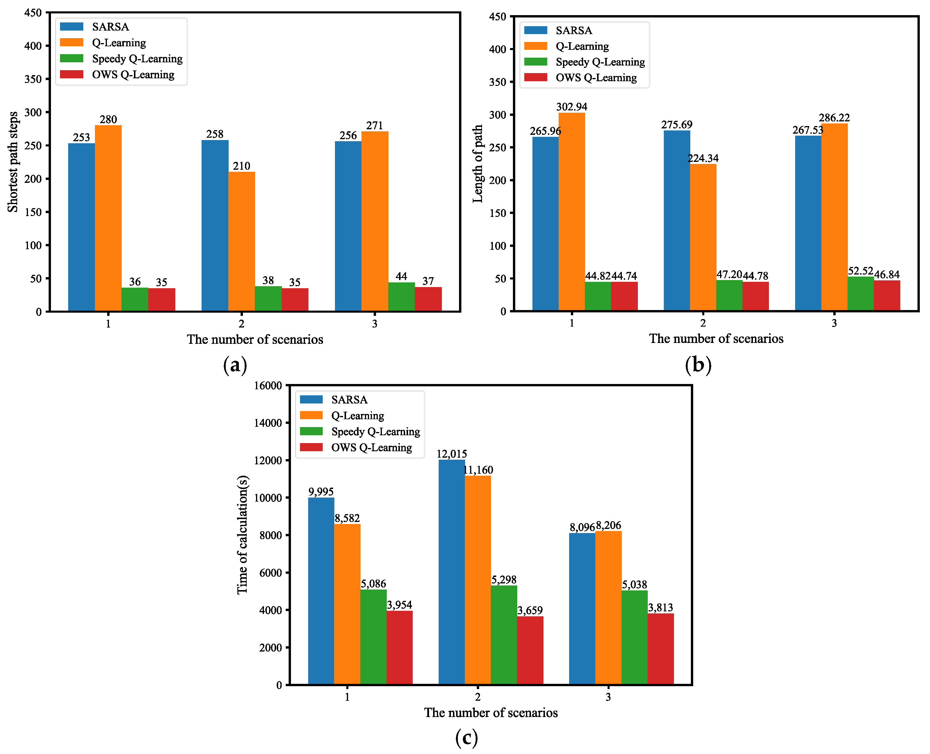
Compare and analyze the experimental results in different scenarios. The average shortest path steps are shown in Figure 12a, the average path length is shown in Figure 12b, and the average calculation time is shown in Figure 12c.

From the histogram (a) of Figure 12, in the simulation experiments of scenarios 1, 2, and 3, the average shortest path steps of UGVs under the OWS Q-learning algorithm in the path planning process is less than the average shortest path steps under the SARSA algorithm, Q-learning algorithm, and speedy Q-learning algorithm. The histogram (b) shows that under the three experimental scenarios, the average length of the path planned by the OWS Q-learning algorithm is the shortest. The histogram (c) shows that under different experimental scenarios, the OWS Q-learning algorithm takes the shortest time to perform path planning and has the highest problem-solving efficiency. Specifically, the improvement in the calculation time of the OWS Q-learning algorithm compared to the SARSA algorithm, Q-learning algorithm, and speedy Q-learning algorithm is shown in

Table 6. The improvement in calculation time of the OWS Q-learning algorithm compared to other algorithms.

Scenario	Statistics	SARSA	Q-Learning	Speedy Q-Learning
1	Calculation time	60.44%	53.93%	22.26%
2	Calculation time	69.55%	67.21%	30.94%
3	Calculation time	52.90%	53.53%	24.32%

.

The convergence performance of the four algorithms in different experimental scenarios and the results of the average reward are integrated into

Table 7. Performance comparison of the four algorithms.

Scenario	Number of Iterations	Evaluation Indicators	SARSA	Q-Learning	Speedy Q-Learning	OWS Q-Learning
1	1800	Astringency	Divergent	Divergent	Divergent	1010 iterations begin to converge
		Average reward	—	—	—	8
2	1800	Astringency	Divergent	Divergent	Divergent	858 iterations begin to converge
		Average reward	—	—	—	12
3	1800	Astringency	Divergent	Divergent	Divergent	810 iterations begin to converge
		Average reward	—	—	—	15

.

From the results of Table 6, the SARSA algorithm, Q-learning algorithm, and speedy Q-learning algorithm do not converge in the simulation experiments in the three scenarios. The OWS Q-learning algorithm proposed in this paper can achieve a convergence effect in the simulation experiments of three scenarios.

Based on the above result analysis, the OWS Q-learning algorithm proposed in this paper is superior to SARSA, Q-learning, and speedy Q-learning algorithms in terms of path selection, algorithm convergence, and calculation time.

6. Conclusions and Outlook

In order to promote the intelligent development of parks, based on the low execution efficiency of single UGV tasks, the slow convergence speed of Q-learning algorithms in multi-agent systems and complex environments, and the low learning efficiency, this paper proposes a collision avoidance cooperation mechanism among multiple UGV and an improved reinforcement learning algorithm—OWS Q-learning algorithm. Based on the idea of the Q-learning algorithm, the OWS Q-learning algorithm changes the update mode of Q function, the learning rate α and the $\epsilon -greedy$ strategy of action selection. Finally, simulation experiments are conducted in three different scenarios, and the performance of the proposed OWS Q-learning is compared with SARSA, Q-learning, and speedy Q-learning. Compared with the experimental results of the other three algorithms, only the OWS Q-learning algorithm can converge, and the OWS Q-learning algorithm has planned the shortest collision-free path for UGVS in different experimental scenarios. In experimental scenario 1, compared with SARSA, Q-learning, and speedy Q-learning, the calculation time of OWS Q-learning was reduced by 60.44%, 53.93%, and 22.26%, respectively. In experimental scenario 2, compared with the above three algorithms, the calculation time of OWS Q-learning is reduced by 69.55%, 67.21%, and 30.94%, respectively. In experimental scenario 3, compared with the above three algorithms, the calculation time of OWS Q-learning is reduced by 52.90%, 53.53%, and 24.32%, respectively.

The OWS Q-learning algorithm is verified to be superior to the comparison algorithm. The multi-UGV collision avoidance coordination mechanism proposed in this manuscript is based on the static environment of the park, but in real life, emergencies may occur in the park, such as sudden pedestrians, vehicles, etc., which will involve some dynamically changing obstacles, and the environment will become more complex. Therefore, in the face of a random environment, this collision avoidance coordination mechanism needs to be further improved, and the OWS Q-learning algorithm needs to be further improved to better handle a larger number of UGVs. In future research work, on the one hand, we will consider the dynamic complex environment in the park, consider the existence of dynamic obstacles in the designed multi-UGV collision avoidance coordination mechanism, on the other hand, in order to further improve the performance of the OWS Q-learning algorithm, we will consider the research and improvement from the structural framework of the algorithm to better solve the path planning problem of multiple UGVs in more complex environments.