Mathematical Analysis of an Anthroponotic Cutaneous Leishmaniasis Model with Asymptomatic Infection

Abstract

This work aims mainly to study the impact of experiencing asymptomatic anthroponotic cutaneous leishmaniasis (ACL) infection on the overall dynamics and outcomes of the disease. Therefore, a deterministic model for the transmission dynamics of ACL of type SEAIS in the human host and SI in sandfly populations is proposed and mathematically analyzed. The model is shown to be well-posed. Its equilibrium and stability analyses are shown. The equilibrium analysis shows that the model has an ACL-free equilibrium that is proven to be locally and globally asymptotically stable if and only if ${\mathcal{R}}_0<1$. In addition, the model has a unique ACL-endemic equilibrium that is shown to exist and be locally asymptotically stable if and only if ${\mathcal{R}}_0>1$. Numerical simulations are performed to show the asymptotic stability of these equilibriums. In addition, the effect of ignoring asymptomatic infections is studied and the analysis shows that ignoring the development of asymptomatic infections overestimates the effort required to eliminate the infection. Moreover, it implies inaccurate measures of controlling ACL infection, especially those based on either using insecticide sprays or bednets.

1. Introduction

Cutaneous leishmaniasis (CL) is a neglected vector-borne disease spread in tropical and subtropical regions. It is spread mainly through the bite of an infected female sandfly while taking its meal from the definitive host. Although there has been a successful reduction in its burden, CL disease remains a public health challenge, as it is endemic in about ninety countries worldwide [1]. It is estimated that the yearly global incidence of CL ranges from 0.6 million to one million cases. Throughout the last decade, the disease has had various emerging outbreaks in different parts of the world [2]. Most of the cases occur in the Americas, the Mediterranean basin, the Middle East, and Central Asia [3]. Even in some countries, where CL is endemic, the disease is focused in certain parts/regions of them [4]. CL could either be anthroponotic (referred to by ACL) or zoonotic (referred to by ZCL). Both types have different clinical features, diverse epidemiological characteristics, and different etiological agents. For example, the main etiological agent of ZCL is Leishmania major, while that of ACL is Leishmania tropica [5]. In this work, we are interested in studying the spread dynamics of ACL, with an approach based on the use of a deterministic differential equations model on the population level.

Various studies have been published to increase knowledge on the transmissibility and controllability of leishmaniasis diseases. For example, Zhao et al. [6] developed and analyzed a mathematical model of type SEIHR in humans, SEI in sandflies, and SEIR in dogs to study the dynamics of zoonotic visceral leishmaniasis (ZVL) in Brazil. However, Bi et al. [7] extended the SEIR -SEI-SEIHR zoonotic visceral leishmaniasis model to include age structure (i.e., partial differential equation model) in the human host. Other mathematical modeling studies on visceral leishmaniasis include the works of Barley et al. [8], Hussaini et al. [9], Kaabi and Zhioua [10], and those considered in the review article of Rock et al. [11].

Mathematical models have been used to study the transmission dynamics of cutaneous leishmaniasis too. For example, Chaves and Hernandez [12] introduced and analyzed a mathematical model for the spread of American cutaneous leishmaniasis. The authors presented and analyzed an SIS model in three populations (humans, reservoir, and sandfly populations) and obtained expressions that allow computing threshold conditions for the persistence of the infection. However, Bacaêr and Guernaoui [13] developed a mathematical model that considers the vector population’s seasonality and the distribution of the latent period from infection to symptoms in humans. In addition, Barradas and Caja Rivera [14] introduced and analyzed a vector–host model (of type SIR in humans and SEI in the vector populations) for describing the dynamics of vector-borne diseases, with special application to the case of cutaneous leishmaniasis in Peru. Zamir et al. [15] presented a mathematical model of type SEIR in humans and SEI in the vector to describe the dynamics of ACL. The authors found the basic reproduction number of the model and analyzed its sensitive dependence on the model parameters. Then, they introduced some control parameters in the basic model and found the optimal control, taking into account the lowest cost. Other studies include those published by De Almeida et al. [16], Agyingi et al. [17], Biswas et al. [18], and the references therein.

The life cycle of ACL has two stages, namely, the human stage and the sandfly stage. Briefly, susceptible sandflies become infected when they bite a CL-infected human to feed on his/her blood. However, susceptible humans acquire ACL infection while an infected female sandfly takes its meal from a susceptible human. It is worth mentioning that humans acquire the infection and become latent, where they neither transmit the infection nor show symptoms of ACL. Those latent individuals may develop symptoms and become infected where they can transmit the infection to susceptible sandflies. However, it is evident that some people have a silent ACL infection, without any symptoms or signs [19]. Humans who develop clinical evidence of ACL infection have at least one sore on their skin. The ACL sores usually develop within a few weeks or months of the sandfly bite. They usually heal on their own, even without treatment, but they may last for months or even years. However, humans may acquire ACL infection more than once. Therefore, a mathematical model of type SEIS (susceptible–exposed–infected–susceptible) in humans would be appropriate to develop and use in describing ACL transmission dynamics.

In this work, we extend the previous works and take into account both the asymptomatic infections and the repeated infections, in the sense that human individuals may acquire the ACL infection more than once. Therefore, we introduce a model of type SEAIS in the human population. As the life expectancy of sandflies is very short compared to that of humans, we assume an SI model for the sandfly population. The model is described and formulated in Section 2. In Section 3, the equilibrium analysis is shown and the basic reproduction number is computed. The local stability of the equilibriums is established in Section 4. In Section 5, numerical simulations for the model with randomly selected initial conditions are used to numerically show the global stability of the equilibriums. The impact of ignoring the asymptomatic infection on ACL disease outcomes is shown in Section 6. A summary and conclusion are given in Section 7.

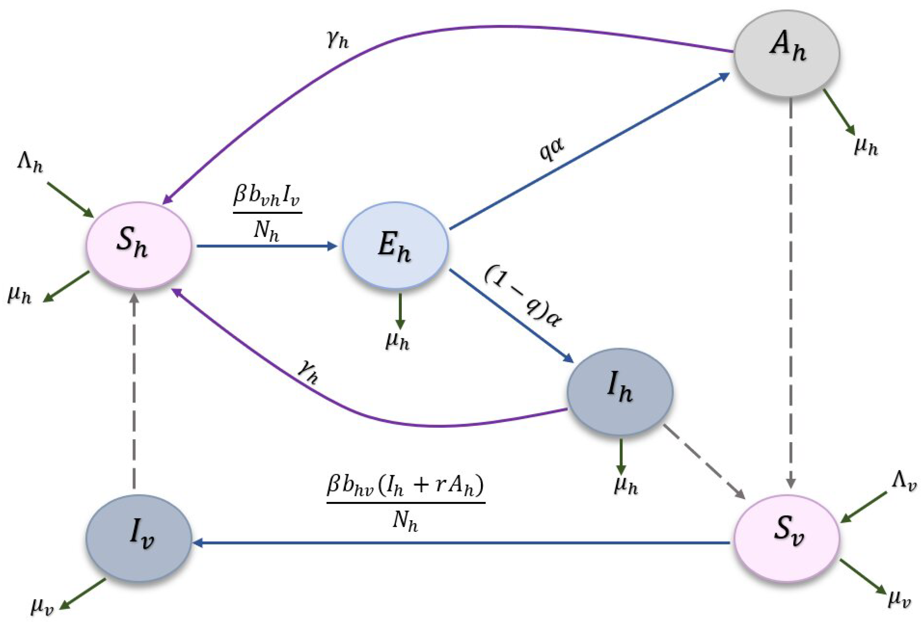
2. Model Formulation and Its Basic Properties

As we model the anthroponotic cutaneous leishmaniasis, we consider both human and sandfly populations. The total human population is split into four mutually independent categories: susceptible, exposed, asymptomatic infected, and symptomatic infected individuals. Their size at time t is denoted by $S_h\left(t\right)$, $E_h\left(t\right)$, $A_h\left(t\right)$, and $I_h\left(t\right)$, respectively. However, the sandfly population is subdivided into susceptible (with size $S_v\left(t\right)$) and infected (with size $I_v\left(t\right)$) sandflies. Susceptible humans are assumed to recruit at the rate ${\Lambda }_h$ and die naturally at the rate ${\mu }_h$. They acquire CL infection, and become exposed, due to being bitten by infected sandflies at the infection rate ${\lambda }_{vh}\left(t\right)$, where

$${\lambda }_{vh}\left(t\right)=\beta \times b_{vh}\times {\displaystyle \frac{I_v}{N_h}}.$$

Exposed humans are not capable of transmitting CL infection to susceptible sandflies, but they are assumed to leave their exposed status either by natural death at the rate ${\mu }_h$ or developing CL infection status at rate $\alpha$, where it is assumed that a proportion q of them become asymptomatic, while the other proportion ($1-q$) develop symptoms and become symptomatic infected. Both asymptomatic and symptomatic infected individuals are assumed to die naturally at the rate ${\mu }_h$ and recover with temporal immunity at the rate ${\gamma }_h$.

The sandfly population is assumed to be recruited (susceptible) at the rate ${\Lambda }_v$ and die naturally at the rate ${\mu }_v$. Susceptible sandflies acquire CL infection at a rate ${\lambda }_{hv}$ and become infected while taking their meals from either or both the symptomatic and asymptomatic infected humans, where

$${\lambda }_{hv}=\beta \times b_{hv}\times {\displaystyle \frac{(I_h+r{A}_h)}{N_h}}.$$

A schematic diagram for the transition and interaction between the various model states is shown in Figure 1, while the physical meaning of the model states and parameters is summarized in

Table 1. Description of state variables and parameters for model (1).

State Variables and Parameters	Description
$S_h$	Number of susceptible humans at time t.
$E_h$	Number of exposed humans in the latent period at time t.
$A_h$	Number of asymptomatic humans (infected but without noticeable disease and infectious ) at time t.
$I_h$	Number of infected humans at time t.
$S_v$	Number of susceptible sandflies at time t.
$I_v$	Number of infectious sandflies at time t.
$N_h$	Total human population size at time t.
$N_v$	Total sandflies population size at time t.
${\Lambda }_h$	Recruitment rate of humans.
${\Lambda }_v$	Recruitment rate of sandflies.
${\mu }_h$	Natural death rate of humans.
${\mu }_v$	Natural death rate of sandflies.
${\gamma }_h$	Recovery rate (with temporal immunity) from symptomatic/asymptomatic cutaneous Leishmaniasis (CL) infection.
$\alpha$	The rate at which human individuals leave the exposed state.
$\beta$	The rate at which sandflies bite the body of human individuals.
q	The probability that an exposed human develops asymptomatic CL infection after leaving the incubation period.
r	The relative transmissibility of asymptomatic with respect to symptomatic CL infection.
$b_{hv}$	The probability at which a susceptible sandfly acquires CL infection while taking its meal from a CL-infected human.
$b_{vh}$	The probability at which a susceptible human acquires CL infection while being bitten by a CL-infected sandfly.

.

The mathematical representation of the model is given by

$$\begin{array}{ccc}\hfill {\displaystyle \frac{d{S}_h}{dt}}& =& {\Lambda }_h-\frac{\beta b_{vh}{I}_v{S}_h}{N_h}-{\mu }_h{S}_h+{\gamma }_h(A_h+I_h),\hfill \\ \hfill {\displaystyle \frac{d{E}_h}{dt}}& =& \frac{\beta b_{vh}{I}_v{S}_h}{N_h}-(\alpha +{\mu }_h)E_h,\hfill \\ \hfill {\displaystyle \frac{d{A}_h}{dt}}& =& q\alpha E_h-({\mu }_h+{\gamma }_h)A_h,\hfill \\ \hfill {\displaystyle \frac{d{I}_h}{dt}}& =& (1-q)\alpha E_h-({\mu }_h+{\gamma }_h)I_h,\hfill \\ \hfill {\displaystyle \frac{d{S}_v}{dt}}& =& {\Lambda }_v-{\displaystyle \frac{\beta b_{hv}(I_h+r{A}_h)S_v}{N_h}}-{\mu }_v{S}_v,\hfill \\ \hfill {\displaystyle \frac{d{I}_v}{dt}}& =& {\displaystyle \frac{\beta b_{hv}(I_h+r{A}_h)S_v}{N_h}}-{\mu }_v{I}_v\hfill \end{array}$$

(1)

so that all parameters are positive and as defined in

Table 2. Model (1) parameters and their baseline and references.

Parameter	Value	Range	Unit	Reference
${\Lambda }_h$	12,327	–	Per week	[20]
${\Lambda }_v$	112	[35–350]	Per week	[14,21]
${\mu }_h$	$1/(75.5\times 52)$	–	Per week	[20]
${\mu }_v$	0.0945	[0.077, 0.525]	Per week	[14,22]
${\gamma }_h$	0.0006391	[0.0000791–0.004991]	Per week	[14,21]
$\alpha$	0.33	[0.125, 0.5]	Per week	[23]
$\beta$	0.48146	[4.1944–18.7754]	Per week	[14,21]
q	0.1	–	Dimensionless	Assumed
r	0.3	–	Dimensionless	Assumed
$b_{hv}$	0.0097	[0.0028–0.08]	Dimensionless	[14,21]
$b_{vh}$	0.7198	[0.08–0.9]	Dimensionless	[14]

. As $N_h=S_h+E_h+A_h+I_h$ and $N_v=S_v+I_v$, then by adding the first four equations of (1), we obtain the following equation:

$${\displaystyle \frac{d{N}_h}{dt}}={\Lambda }_h-{\mu }_h{N}_h.$$

(2)

Its solution is

$$N_h\left(t\right)={\displaystyle \frac{{\Lambda }_h}{{\mu }_h}}+\left(N_h\left(0\right)-{\displaystyle \frac{{\Lambda }_h}{{\mu }_h}}\right)e^{-{\mu }_{h}t}.$$

(3)

Similarly, we add the last two equations of (1) to obtain the following equation:

$${\displaystyle \frac{d{N}_v}{dt}}={\Lambda }_v-{\mu }_v{N}_v$$

(4)

which has the solution

$$N_v\left(t\right)={\displaystyle \frac{{\Lambda }_v}{{\mu }_v}}+\left(N_v\left(0\right)-{\displaystyle \frac{{\Lambda }_v}{{\mu }_v}}\right)e^{-{\mu }_{v}t}.$$

(5)

Both solutions indicate that $N_h\left(t\right),N_v\left(t\right)>0$, and when t tends to ∞, then the pair $(N_h\left(t\right),N_v\left(t\right))$ tends to $({\Lambda }_h/{\mu }_h,{\Lambda }_v/{\mu }_v)$. Hence, the appropriate closed set $\Omega$ on which model (1) along with (2) is defined reads

$$\begin{array}{ccc}\hfill \Omega & =& {\Omega }_h\cup {\Omega }_v\in {\mathbb{R}}_{+}^4\times {\mathbb{R}}_{+}^2,\hfill \\ \hfill {\Omega }_h& =& \left\{(S_h,E_h,A_h,I_h)\in {\mathbb{R}}_{+}^4,0\le S_h+E_h+A_h+I_h\le {\Lambda }_h/{\mu }_h\right\},\hfill \\ \hfill {\Omega }_v& =& \left\{(S_v,I_v)\in {\mathbb{R}}_{+}^2,0\le S_v+I_v\le {\Lambda }_v/{\mu }_v\right\}.\hfill \end{array}$$

(6)

It is easy to check that the right-hand side of each equation in the model (1) is a continuous function in the model state variables. Moreover, their partial derivatives (see Appendix A) do exist and are continuous, too. Therefore, they are locally Lipschitz. Hence, any solution, of model (1), starting with initial conditions $(S_h\left(0\right),E_h\left(0\right),A_h\left(0\right),I_h\left(0\right))\in {\Omega }_h$ and $(S_v\left(0\right),I_v\left(0\right))\in {\Omega }_v$ is unique. Appendix B shows the proof of the following proposition on the positivity and boundedness of the solutions.

Proposition 1. 

The closed set Ω is positively invariant along with (1).

It is worth mentioning that the positive invariance property of the set $\Omega$ could be proven by applying lemma 1 of Valle et al. [24] and also by following the approach shown in more detail in section II.A of De Leenheer and Aeyels [25].

3. Equilibrium Analysis and the Basic Reproduction Number

As model (1) is nonlinear, exact time-dependent solutions are impossible to derive, but the qualitative behavior of the solutions could be studied by analyzing the equilibrium. To this end, the derivatives in the left-hand side of (1) are set equal to zero and we solve the remaining nonlinear algebraic system in the state variables. At equilibrium, the $A_h$ and $I_h$ equations in (1) imply that

$$\begin{array}{ccc}\hfill A_h& =& {\displaystyle \frac{q\alpha E_h}{({\mu }_h+{\gamma }_h)}},\hfill \end{array}$$

(7)

$$\begin{array}{ccc}\hfill I_h& =& {\displaystyle \frac{(1-q)\alpha E_h}{({\mu }_h+{\gamma }_h)}}.\hfill \end{array}$$

(8)

Hence,

$$I_h+r{A}_h={\displaystyle \frac{[(1-q)+rq]\alpha E_h}{({\mu }_h+{\gamma }_h)}}.$$

(9)

However, the equilibrium $I_v$ equation in (1) implies that

$$I_h+r{A}_h={\displaystyle \frac{{\mu }_v{I}_v{N}_h}{\beta b_{hv}{S}_v}}.$$

(10)

Hence, from (9) and (10), we obtain

$${\displaystyle \frac{[(1-q)+rq]\alpha E_h}{({\mu }_h+{\gamma }_h)}}-{\displaystyle \frac{{\mu }_v{I}_v{N}_h}{\beta b_{hv}{S}_v}}=0.$$

(11)

The equilibrium $E_h$ equation in (1) could be rewritten as

$$I_v={\displaystyle \frac{N_h(\alpha +{\mu }_h)E_h}{\beta b_{vh}{S}_h}}.$$

(12)

Substituting from (12) into (11), we obtain

$$\left({\displaystyle \frac{\left(\right(1-q)+rq)\alpha }{({\mu }_h+{\gamma }_h)}}-{\displaystyle \frac{N_h^2{\mu }_v(\alpha +{\mu }_h)}{{\beta }^2{b}_{hv}{b}_{vh}{S}_h{S}_v}}\right)E_h=0.$$

(13)

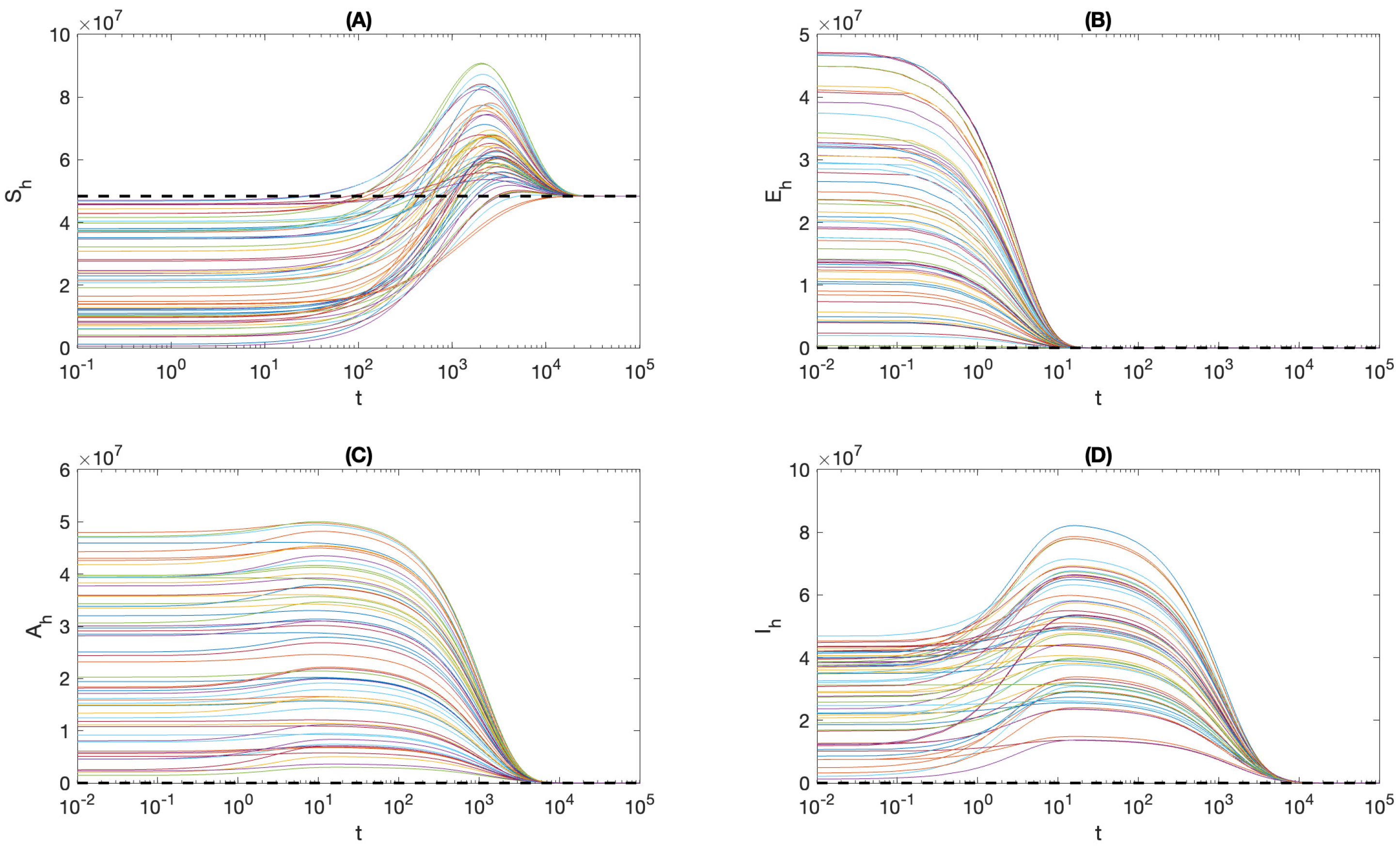
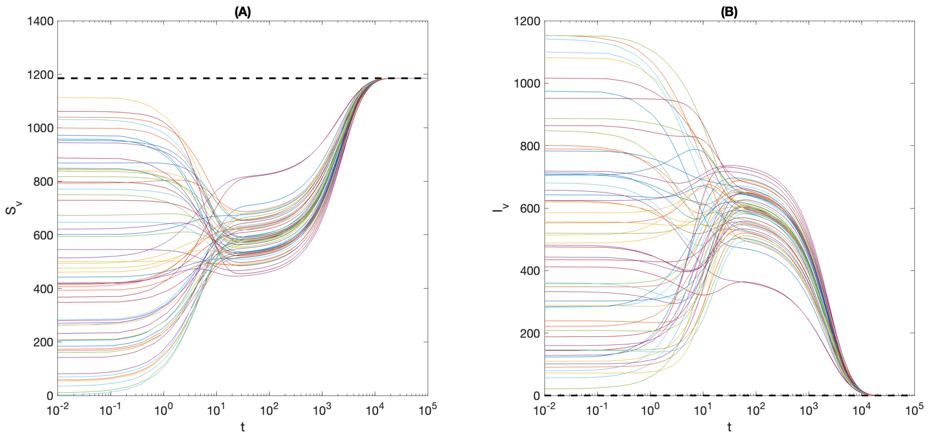
3.1. CL-Free Equilibrium

If $E_h=0$, then Equations (7), (8) and (12) imply that $A_h$, $I_h$, and $I_v=0$, respectively. Therefore, the equilibrium $S_h$ and $S_v$ equations in (1) imply that $S_h={\displaystyle \frac{{\Lambda }_h}{{\mu }_h}}$ and $S_v={\displaystyle \frac{{\Lambda }_v}{{\mu }_v}}$. Thus, the CL-free equilibrium reads

$$E_0={\left(S_h^0,E_h^0,A_h^0,I_h^0,S_v^0,I_v^0\right)}^T={\left({\displaystyle \frac{{\Lambda }_h}{{\mu }_h}},0,0,0,{\displaystyle \frac{{\Lambda }_v}{{\mu }_v}},0\right)}^T$$

(14)

where the prime (${}^T$) denotes vector-transpose. Hence, we have the following proposition.

Proposition 2. 

Model (1) has a cutaneous-Leishmaniasis-free equilibrium $E_0$, given by (14).

3.2. The Basic Reproduction Number

The basic reproduction number is computed by following the general approach shown in van den Driessche and Watmough [26]. We first determine the vector matrices of new incidences $\mathcal{F}$ and transfer terms $\mathcal{V}$ from the four equations of infected humans and sandflies (i.e., $E_h,A_h,I_h$, and $I_v$ equations), as

$$\mathcal{F}=\left(\begin{array}{c}\frac{\beta b_{vh}{I}_v{S}_h}{N_h}\\ \\ 0\\ \\ 0\\ \\ {\displaystyle \frac{\beta b_{hv}(I_h+r{A}_h)S_v}{N_h}}\end{array}\right)\mathrm{and}\mathcal{V}=\left(\begin{array}{c}(\alpha +{\mu }_h)E_h\\ \\ ({\mu }_h+{\gamma }_h)A_h-q\alpha E_h\\ \\ ({\mu }_h+{\gamma }_h)I_h-(1-q)\alpha E_h\\ \\ {\mu }_v{I}_v\end{array}\right).$$

Then, the new-infection terms matrix F and the remaining transfer terms matrix V are obtained by, respectively, computing the Jacobian matrices of both $\mathcal{F}$ and $\mathcal{V}$ (with respect to the state variable of infected terms $E_h,A_h,I_h$, and $I_v$) evaluated at the CL-free equilibrium $E_0$ as

$$F=\left(\begin{array}{cccc}0& 0& 0& \beta b_{vh}\\ \\ 0& 0& 0& 0\\ \\ 0& 0& 0& 0\\ \\ 0& {\displaystyle \frac{\beta b_{hv}r{\Lambda }_v{\mu }_h}{{\Lambda }_h{\mu }_v}}& {\displaystyle \frac{\beta b_{hv}{\Lambda }_v{\mu }_h}{{\Lambda }_h{\mu }_v}}& 0\end{array}\right)\mathrm{and}V=\left(\begin{array}{cccc}\alpha +{\mu }_h& 0& 0& 0\\ \\ -q\alpha & {\mu }_h+{\gamma }_h& 0& 0\\ \\ (1-q)\alpha & 0& {\mu }_h+{\gamma }_h& 0\\ \\ 0& 0& 0& {\mu }_v\end{array}\right).$$

Hence, the basic reproduction number ${\mathcal{R}}_0$ is the dominant eigenvalue of the next generation matrix $F{V}^{-1}$ and is given by

$${\mathcal{R}}_0=\sqrt{{\displaystyle \frac{\beta b_{vh}}{{\mu }_v}}\times {\displaystyle \frac{\beta b_{hv}}{{\gamma }_h+{\mu }_h}}\times {\displaystyle \frac{\alpha }{\alpha +{\mu }_h}}\times {\displaystyle \frac{{\Lambda }_v/{\mu }_v}{{\Lambda }_h/{\mu }_h}}\times \left(1-(1-r)q\right)}.$$

(15)

In summary, we show the following proposition.

Proposition 3. 

The basic reproduction number ${\mathcal{R}}_0$ of model (1) is given by Formula (15).

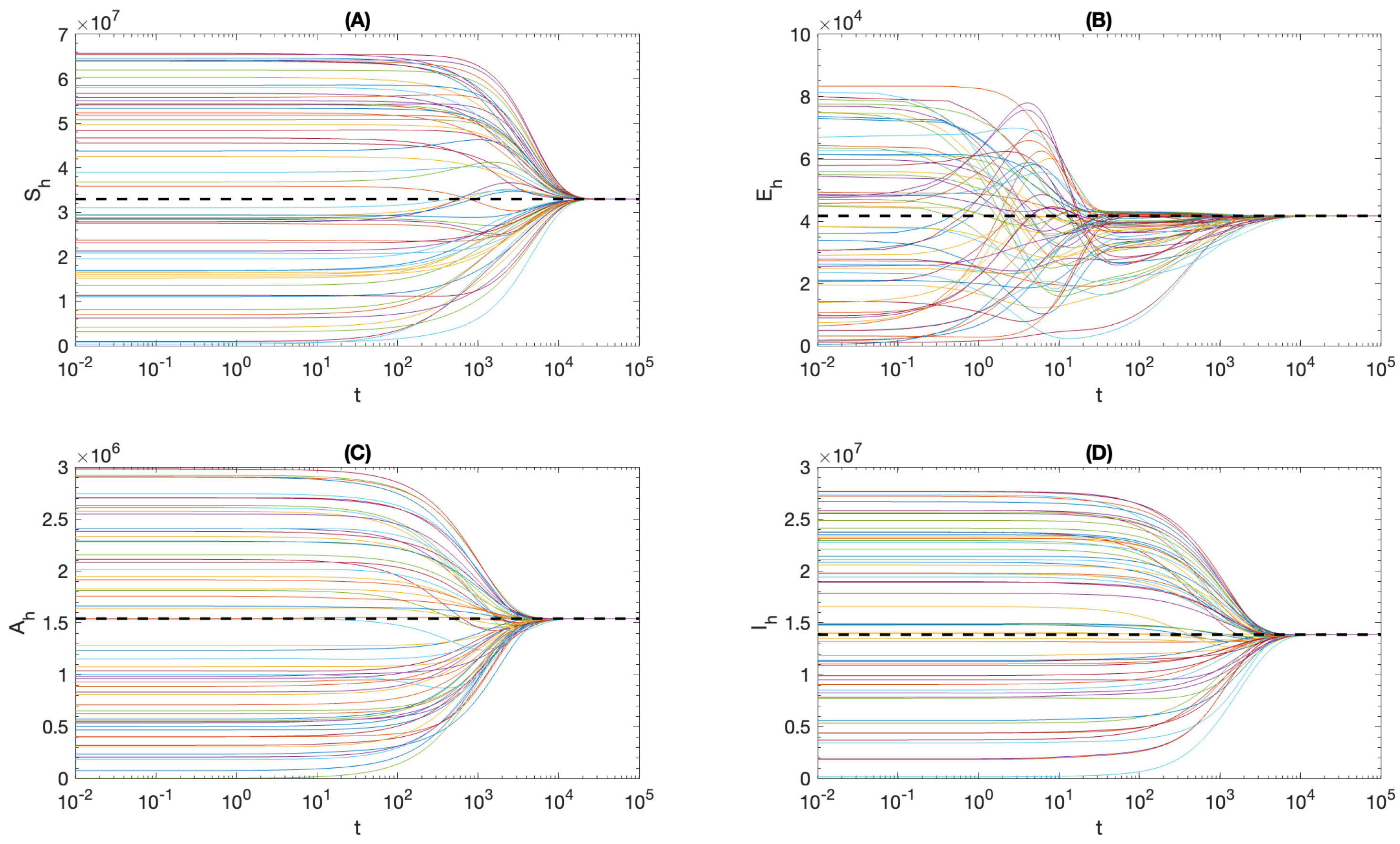
3.3. Endemic Equilibrium

If $E_h\ne 0$, then Equation (13) implies that

$$S_v={\displaystyle \frac{N_h^2{\mu }_v(\alpha +{\mu }_h)({\mu }_h+{\gamma }_h)}{{\beta }^2{b}_{hv}{b}_{vh}[(1-q)+rq]\alpha S_h}}.$$

(16)

It is worth mentioning that, throughout the rest of the current subsection, $N_h$ denotes the human population size at equilibrium and equals ${\Lambda }_h/{\mu }_h$. By substituting Equation (12) into the equilibrium $S_h$-equation in (1), we obtain

$$0={\Lambda }_h-(\alpha +{\mu }_h)E_h-{\mu }_h{S}_h+{\gamma }_h(A_h+I_h).$$

(17)

Now, we use (7) and (8) in (17) and simplify to obtain

$$\begin{array}{c}\hfill E_h={\displaystyle \frac{({\Lambda }_h-{\mu }_h{S}_h)({\mu }_h+{\gamma }_h)}{{\mu }_h(\alpha +{\mu }_h+{\gamma }_h)}}.\end{array}$$

(18)

In addition, using (10) and (16) in the equilibrium $S_v$-equation in (1), we obtain

$${\Lambda }_v={\mu }_v{I}_v+{\displaystyle \frac{{\mu }_v^2{N}_h^2(\alpha +{\mu }_h)({\mu }_h+{\gamma }_h)}{{\beta }^2{b}_{hv}{b}_{vh}[(1-q)+rq]\alpha S_h}}.$$

(19)

Omitting $I_v$ between (19) and (10) implies that

$${\Lambda }_v={\displaystyle \frac{{\mu }_v{N}_h(\alpha +{\mu }_h)E_h}{\beta b_{vh}{S}_h}}+{\displaystyle \frac{{\mu }_v^2{N}_h^2(\alpha +{\mu }_h)({\mu }_h+{\gamma }_h)}{{\beta }^2{b}_{hv}{b}_{vh}[(1-q)+rq]\alpha S_h}}.$$

(20)

Upon substituting from (18) in (20), we obtain

$${\Lambda }_v={\displaystyle \frac{{\mu }_v{N}_h(\alpha +{\mu }_h)}{\beta b_{vh}{S}_h}}\times {\displaystyle \frac{({\Lambda }_h-{\mu }_h{S}_h)({\mu }_h+{\gamma }_h)}{{\mu }_h(\alpha +{\mu }_h+{\gamma }_h)}}+{\displaystyle \frac{{\mu }_v^2{N}_h^2(\alpha +{\mu }_h)({\mu }_h+{\gamma }_h)}{{\beta }^2{b}_{hv}{b}_{vh}[(1-q)+rq]\alpha S_h}}.$$

(21)

Now, we extract $S_h$ to obtain

$$S_h={\displaystyle \frac{N_h{\mu }_v(\alpha +{\mu }_h)({\mu }_h+{\gamma }_h)\kappa }{\beta b_{hv}\alpha [(1-q)+rq]\zeta }}$$

(22)

where

$$\begin{array}{ccc}\hfill \kappa & =& {\Lambda }_h\beta b_{hv}[(1-q)+rq]\alpha +{\mu }_v{\mu }_h{N}_h(\alpha +{\mu }_h+{\gamma }_h),\hfill \\ \hfill \zeta & =& {\Lambda }_v\beta b_{vh}{\mu }_h(\alpha +{\mu }_h+{\gamma }_h)+{\mu }_v{\mu }_h{N}_h(\alpha +{\mu }_h)({\mu }_h+{\gamma }_h).\hfill \end{array}$$

Upon using (22) in (16) and (18), we obtain

$$\begin{array}{ccc}\hfill S_v& =& {\displaystyle \frac{N_h\zeta }{\beta b_{vh}\kappa }},\hfill \end{array}$$

(23)

$$\begin{array}{ccc}\hfill E_h& =& {\displaystyle \frac{({\mu }_h+{\gamma }_h)\tau }{\beta b_{hv}\alpha [(1-q)+rq]\zeta }}.\hfill \end{array}$$

(24)

where

$$\tau ={\Lambda }_h{\Lambda }_v{\beta }^2{b}_{hv}{b}_{vh}\alpha [(1-q)+rq]-N_h^2{\mu }_v^2{\mu }_h(\alpha +{\mu }_h)({\mu }_h+{\gamma }_h).$$

In addition, we use (24) in (8) and (7) to obtain

$$I_h={\displaystyle \frac{(1-q)\tau }{\beta b_{hv}[(1-q)+rq]\zeta }}\mathrm{and}{A}_h={\displaystyle \frac{q\tau }{\beta b_{hv}[(1-q)+rq]\zeta }}.$$

(25)

From inserting (22) and (24) into (12) we obtain

$$I_v={\displaystyle \frac{\tau }{\beta b_{vh}{\mu }_v\kappa }}.$$

(26)

Hence, the endemic equilibrium is

$$E_e={\left(S_h^e,E_h^e,A_h^e,I_h^e,S_v^e,I_v^e\right)}^T$$

(27)

where

$$\begin{array}{ccc}\hfill S_h^e& ={\displaystyle \frac{N_h{\mu }_v(\alpha +{\mu }_h)({\mu }_h+{\gamma }_h)\kappa }{\beta b_{hv}\alpha [(1-q)+rq]\zeta }},& E_h^e={\displaystyle \frac{({\mu }_h+{\gamma }_h)\tau }{\beta b_{hv}\alpha [(1-q)+rq]\zeta }},\hfill \\ \hfill A_h^e& ={\displaystyle \frac{q\tau }{\beta b_{hv}[(1-q)+rq]\zeta }},& I_h^e={\displaystyle \frac{(1-q)\tau }{\beta b_{hv}[(1-q)+rq]\zeta }},\hfill \\ \hfill S_v^e& ={\displaystyle \frac{N_h\zeta }{\beta b_{vh}\kappa }},& I_v^e={\displaystyle \frac{\tau }{\beta b_{vh}{\mu }_v\kappa }}.\hfill \end{array}$$

(28)

It is noteworthy that $\kappa >0,\zeta >0$, while $\tau >0$ if and only if ${\mathcal{R}}_0>1$. Therefore, we summarize the above result in the following proposition.

Proposition 4. 

Model (1) has a unique endemic equilibrium, given by (27), that exists if and only if the basic reproduction number ${\mathcal{R}}_0>1$.

4. Local Stability Analysis

The local stability analysis of the equilibrium points is established based on the linearization approach (Lyapunov’s first method). Rather than considering model (1), we replace $S_h$ and $S_v$ equations with those of $N_h$ and $N_v$, respectively, and substitute $S_h=N_h-(E_h+A_h+I_h)$ and $S_v=N_v-I_v$ to obtain

$$\begin{array}{ccc}\hfill {\displaystyle \frac{d{N}_h}{dt}}& =& {\Lambda }_h-{\mu }_h{N}_h,\hfill \\ \hfill {\displaystyle \frac{d{E}_h}{dt}}& =& \beta b_{vh}{I}_v\left(1-{\displaystyle \frac{E_h+A_h+I_h}{N_h}}\right)-(\alpha +{\mu }_h)E_h,\hfill \\ \hfill {\displaystyle \frac{d{A}_h}{dt}}& =& q\alpha E_h-({\mu }_h+{\gamma }_h)A_h,\hfill \\ \hfill {\displaystyle \frac{d{I}_h}{dt}}& =& (1-q)\alpha E_h-({\mu }_h+{\gamma }_h)I_h,\hfill \\ \hfill {\displaystyle \frac{d{N}_v}{dt}}& =& {\Lambda }_v-{\mu }_v{N}_v,\hfill \\ \hfill {\displaystyle \frac{d{I}_v}{dt}}& =& {\displaystyle \frac{\beta b_{hv}(I_h+r{A}_h)}{N_h}}(N_v-I_v)-{\mu }_v{I}_v.\hfill \end{array}$$

(29)

Model (29) has generally the Jacobian matrix

$$J=\left(\begin{array}{cccccc}-{\mu }_h& 0& 0& 0& 0& 0\\ \\ J_{21}& J_{22}& {\displaystyle \frac{-\beta b_{vh}{I}_v}{N_h}}& {\displaystyle \frac{-\beta b_{vh}{I}_v}{N_h}}& 0& {\displaystyle \frac{\beta b_{vh}{S}_h}{N_h}}\\ \\ 0& q\alpha & -({\mu }_h+{\gamma }_h)& 0& 0& 0\\ \\ 0& (1-q)\alpha & 0& -({\mu }_h+{\gamma }_h)& 0& 0\\ \\ 0& 0& 0& 0& -{\mu }_v& 0\\ \\ J_{61}& 0& {\displaystyle \frac{r\beta b_{hv}{S}_v}{N_h}}& {\displaystyle \frac{\beta b_{hv}{S}_v}{N_h}}& J_{65}& {\displaystyle \frac{-\beta b_{hv}(I_h+r{A}_h)}{N_h}}-{\mu }_v\end{array}\right)$$

(30)

where

$$\begin{array}{ccc}\hfill J_{21}& =& {\displaystyle \frac{\beta b_{vh}{I}_v(E_h+A_h+I_h)}{N_h^2}},J_{22}=-{\displaystyle \frac{\beta b_{vh}{I}_v(N_h-(E_h+A_h+I_h))}{N_h^2}}-(\alpha +{\mu }_h),\hfill \\ \hfill J_{61}& =& {\displaystyle \frac{-\beta b_{hv}(I_h+r{A}_h)S_v}{N_h^2}},J_{65}={\displaystyle \frac{\beta b_{hv}(I_h+r{A}_h)}{N_h}}.\hfill \end{array}$$

4.1. Local Stability of $E_0$

At the CL-free equilibrium $E_0$, the Jacobian matrix J has the three negative eigenvalues $-{\mu }_h$, $-{\mu }_v,-({\mu }_h+{\gamma }_h)$, in addition to the roots of the characteristic equation

$$a_3{\lambda }^3+a_2{\lambda }^2+a_1\lambda +a_0=0$$

(31)

where

$$\begin{array}{ccc}\hfill a_3& =& 1,\hfill \\ \hfill a_2& =& (\alpha +{\mu }_h)+({\mu }_h+{\gamma }_h)+{\mu }_v,\hfill \\ \hfill a_1& =& (\alpha +{\mu }_h){\mu }_v+({\mu }_h+{\gamma }_h){\mu }_v+(\alpha +{\mu }_h)({\mu }_h+{\gamma }_h),\hfill \\ \hfill a_0& =& {\mu }_v(\alpha +{\mu }_h)({\mu }_h+{\gamma }_h)(1-{\mathcal{R}}_0^2).\hfill \end{array}$$

Based on the Routh–Hurwitz criterion, all roots of the characteristic polynomial (31) have negative real part if and only if all coefficients $a_i,i\in \{0,1,2,3\}$ and the determinants ${\Delta }_1,{\Delta }_2$ are all positive, where ${\Delta }_1=a_2{a}_1-a_0{a}_3$ and ${\Delta }_2=a_0{\Delta }_1$. It is clear that $a_3,a_2,and a_1$ are positive, while $a_0$ is positive if and only if ${\mathcal{R}}_0<1$. Moreover,

$$\begin{array}{ccc}\hfill {\Delta }_1& =& \left((\alpha +{\mu }_h)+({\mu }_h+{\gamma }_h)+{\mu }_v\right)((\alpha +{\mu }_h){\mu }_v+({\mu }_h+{\gamma }_h){\mu }_v\hfill \\ & +& (\alpha +{\mu }_h)({\mu }_h+{\gamma }_h))-{\mu }_v(1-{\mathcal{R}}_0^2)(\alpha +{\mu }_h)({\mu }_h+{\gamma }_h).\hfill \\ & =& (\alpha +{\mu }_h)((\alpha +{\mu }_h){\mu }_v+({\mu }_h+{\gamma }_h){\mu }_v+(\alpha +{\mu }_h)({\mu }_h+{\gamma }_h)\hfill \\ & +& {({\mu }_h+{\gamma }_h)}^2+({\mu }_h+{\gamma }_h){\mu }_v{\mathcal{R}}_0^2)+{({\mu }_h+{\gamma }_h)}^2{\mu }_v>0\forall {\mathcal{R}}_0<1\hfill \end{array}$$

(32)

and

$${\Delta }_2={\mu }_v(1-{\mathcal{R}}_0^2)(\alpha +{\mu }_h)({\mu }_h+{\gamma }_h){\Delta }_1>0\forall {\mathcal{R}}_0<1.$$

(33)

Collecting all together, we obtain the following proposition on the local stability of the CL-free equilibrium.

Proposition 5. 

The CL-free equilibrium $E_0$ is locally asymptotically stable if and only if ${\mathcal{R}}_0<1$.

4.2. Local Stability of the Endemic Equilibrium $E_e$

At the endemic equilibrium, the matrix (30) has the three negative eigenvalues $-{\mu }_v,-{\mu }_h,-({\gamma }_h+{\mu }_h)$, in addition to the roots of the characteristic polynomial

$$c_3{\lambda }^3+c_2{\lambda }^2+c_1\lambda +c_0=0$$

(34)

where

$$\begin{array}{ccc}\hfill c_3& =& 1,\hfill \\ \hfill c_2& =& ({\mu }_h+{\gamma }_h)+(\alpha +{\mu }_h)+{\mu }_v+{\displaystyle \frac{\beta b_{vh}{I}_v}{N_h}}+{\displaystyle \frac{\beta b_{hv}(I_h+r{A}_h)}{N_h}},\hfill \\ \hfill c_1& =& ({\mu }_h+{\gamma }_h)\left((\alpha +{\mu }_h)+{\mu }_v+{\displaystyle \frac{\beta b_{vh}{I}_v}{N_h}}+{\displaystyle \frac{\beta b_{hv}(I_h+r{A}_h)}{N_h}}\right)\hfill \\ & +& \left(\alpha +{\mu }_h+{\displaystyle \frac{\beta b_{vh}{I}_v}{N_h}}\right)\left({\mu }_v+{\displaystyle \frac{\beta b_{hv}(I_h+r{A}_h)}{N_h}}\right)+{\displaystyle \frac{\beta b_{vh}{I}_v}{N_h}}\alpha ,\hfill \\ \hfill c_0& =& {\displaystyle \frac{\beta b_{hv}(I_h+r{A}_h)}{N_h}}\left(({\mu }_h+{\gamma }_h)(\alpha +{\mu }_h)+{\displaystyle \frac{\beta b_{vh}{I}_v}{N_h}}({\mu }_h+{\gamma }_h+\alpha )\right)\hfill \\ & +& {\displaystyle \frac{\beta b_{vh}{I}_v}{N_h}}({\mu }_h+{\gamma }_h+\alpha ){\mu }_v.\hfill \end{array}$$

It is clear that all coefficients $c_i,i\in \{0,1,2,3\}$ are positive. Therefore, the Routh–Hurwitz criterion implies that the endemic equilibrium $E_e$ is locally asymptotically stable if and only if the determinant ${\tilde{\Delta }}_1=c_2{c}_1-c_0{c}_3$ is positive. Appendix C shows that ${\tilde{\Delta }}_1>0$. Thus, $E_e$ is locally asymptotically stable wherever it exists. In summary, we have the following result.

Proposition 6. 

The CL-endemic equilibrium $E_e$ is locally asymptotically stable wherever it exists.

5. Global and Asymptotic Stability

The global stability of the CL-free equilibrium (for ${\mathcal{R}}_0<1$) is proven by following the general approach shown in Section 3 of Castillo-Chavez et al. [27], see also Section 3.4 of [28]. To this end, model (1) is rewritten as

$${\displaystyle \frac{dx}{dt}}=F_1(x,\mathbf{y})\mathrm{and}{\displaystyle \frac{dy}{dt}}=G_1(x,\mathbf{y})$$

(35)

where

$$x={(S_h,S_v)}^T,\mathbf{y}={(E_h,A_h,I_h,I_v)}^T$$

and

$$F_1=\left(\begin{array}{c}{\Lambda }_h-\frac{\beta b_{vh}{I}_v{S}_h}{N_h}-{\mu }_h{S}_h+{\gamma }_h(A_h+I_h)\\ \\ {\Lambda }_v-{\displaystyle \frac{\beta b_{hv}(I_h+r{A}_h)S_v}{N_h}}-{\mu }_v{S}_v\end{array}\right)\mathrm{and}{G}_1=\left(\begin{array}{c}\frac{\beta b_{vh}{I}_v{S}_h}{N_h}-(\alpha +{\mu }_h)E_h\\ \\ q\alpha E_h-({\mu }_h+{\gamma }_h)A_h\\ \\ (1-q)\alpha E_h-({\mu }_h+{\gamma }_h)I_h\\ \\ {\displaystyle \frac{\beta b_{hv}(I_h+r{A}_h)S_v}{N_h}}-{\mu }_v{I}_v\end{array}\right).$$

The components of $x\in {\mathbb{R}}_{+}^2$ denote the uninfected subpopulations, and those of $\mathbf{y}\in {\mathbb{R}}_{+}^4$ denote the infected subpopulations. The CL-free equilibrium $E_0$ is equivalent with $x=x^{\ast }={({\Lambda }_h/{\mu }_h,{\Lambda }_v/{\mu }_v)}^T$ and $\mathbf{y}=\mathbf{O}={(0,0,0,0)}^T$. The approach is based on proving the following two conditions:

(H1) 

For ${\displaystyle \frac{dx}{dt}}=F_1(x,\mathbf{O}),x^{\ast }$ is globally asymptotically stable.

(H2) 

$G_1(x,y)=B\mathbf{y}-\widehat{G}(x,\mathbf{y}),\widehat{G}(x,\mathbf{y})\ge 0$ for $(x,\mathbf{y})\in \Omega$.

Here, $B=D_{\mathbf{y}}{G}_1(x^{\ast },\mathbf{O})$ is an M-matrix. The condition H1 is proved by considering the following Lyapunov function:

$$V(S_h,S_v)=S_h-{\displaystyle \frac{{\Lambda }_h}{{\mu }_h}}-{\displaystyle \frac{{\Lambda }_h}{{\mu }_h}}ln\left({\displaystyle \frac{S_h}{{\Lambda }_h/{\mu }_h}}\right)+S_v-{\displaystyle \frac{{\Lambda }_v}{{\mu }_v}}-{\displaystyle \frac{{\Lambda }_v}{{\mu }_v}}ln\left({\displaystyle \frac{S_v}{{\Lambda }_v/{\mu }_v}}\right).$$

Clearly, $V(S_h,S_v)\ge 0$ along the solution of the system

$${\displaystyle \frac{d}{dt}}{(S_h,S_v)}^T={\left({\Lambda }_h-{\mu }_h{S}_h,{\Lambda }_v-{\mu }_v{S}_v\right)}^T$$

(36)

and is zero if and only if ${(S_h,S_v)}^T={({\Lambda }_h/{\mu }_h,{\Lambda }_v/{\mu }_v)}^T$. In addition, the time-derivative of V, computed along the solution of the system (36), is

$${\displaystyle \frac{d}{dt}}V=-{\mu }_h{S}_h{\left(1-{\displaystyle \frac{{\Lambda }_h}{{\mu }_h{S}_h}}\right)}^2-{\mu }_v{S}_v{\left(1-{\displaystyle \frac{{\Lambda }_v}{{\mu }_v{S}_v}}\right)}^2<0.$$

Therefore, $x^{\ast }={({\Lambda }_h/{\mu }_h,{\Lambda }_v/{\mu }_v)}^T$ is globally stable. This proves condition H1.

To prove condition H2, we rewrite the vector-matrix $G_1(x,\mathbf{y})$ as $B\mathbf{y}-\widehat{G}(x,\mathbf{y}),\widehat{G}(x,\mathbf{y})\ge 0$, where

$$B=D_{\mathbf{y}}{G}_1(x^{\ast },\mathbf{O})=\left(\begin{array}{cccc}-(\alpha +{\mu }_h)& 0& 0& \beta b_{vh}\\ \\ q\alpha & -({\mu }_h+{\gamma }_h)& 0& 0\\ \\ (1-q)\alpha & 0& -({\mu }_h+{\gamma }_h)& 0\\ \\ 0& {\displaystyle \frac{r\beta b_{hv}{\Lambda }_v{\mu }_h}{{\Lambda }_h{\mu }_v}}& {\displaystyle \frac{\beta b_{hv}{\Lambda }_v{\mu }_h}{{\Lambda }_h{\mu }_v}}& -{\mu }_v\end{array}\right)$$

is an M-matrix (where its off-diagonal elements are non-negative) and

$$\widehat{G}(x,\mathbf{y})={\left(\beta b_{vh}{I}_v\left(1-{\displaystyle \frac{S_h}{N_h}}\right),0,0,\beta b_{hv}(I_h+r{A}_h){\displaystyle \frac{{\Lambda }_v/{\mu }_v}{{\Lambda }_h/{\mu }_h}}\left(1-{\displaystyle \frac{S_v}{{\Lambda }_v/{\mu }_v}}\times {\displaystyle \frac{{\Lambda }_h/{\mu }_h}{N_h}}\right)\right)}^T.$$

Therefore, we show the following proposition.

Proposition 7. 

The CL-free equilibrium $E_0$ is globally stable if and only if ${\mathcal{R}}_0<1$.

The asymptotic stability analysis of both the CL-free and CL-endemic equilibriums is established numerically. To this end, the function ode45 in Matlab, which is based on the Runge–Kutta method of order four, is employed to numerically solve model (1) with parameter values as presented in Table 2 and with various randomly generated initial conditions lying in the set $\Omega$. Extensive simulations are performed with a $\beta$ value corresponding to ${\mathcal{R}}_0=0.8<1$ and the simulations are shown in Figure 2 and Figure 3. The figures show that if we start the solutions with any initial values lying in the domain $\Omega$, the number of exposed, asymptomatic, and infected humans and infected sandflies approach zero in the long time run, while those of noninfected humans and sandflies tend to their level at the CL-free equilibrium. In other words, all trajectory solutions are attracted by the CL-free equilibrium. It is worth mentioning that the horizontally broken lines represent the equilibrium solutions.

Similarly, model (1) is extensively and numerically solved with a value of $\beta$ such that ${\mathcal{R}}_0=1.83>1$, and the simulations are shown in Figure 4 and Figure 5. These two figures show that for any initial values of the human and sandfly subpopulations (lying in the set $\Omega$) and for a combination of model parameters chosen such that ${\mathcal{R}}_0>1$, the size of the time-dependent exposed, asymptomatic, and infected human subpopulations and infected sandfly subpopulation will eventually approach a positive level (their levels at the CL-endemic situation) and, hence, the infection persists in both human and sandfly populations. Definitely, the CL-endemic equilibrium attracts all model solutions for values of ${\mathcal{R}}_0>1$. Thus, motivated by the above results, the CL-free equilibrium is asymptotically stable if and only if ${\mathcal{R}}_0<1$, while the CL-endemic equilibrium is asymptotically stable wherever it exists.

It is noteworthy that our in silico simulations (see Colquitt et al. [29]) show the existence of two scenarios for the evolution of the infection; either the infection dies out from both human and sandfly populations (see Figure 2 and Figure 3, respectively), or it persists in both populations (see Figure 4 and Figure 5). The first scenario is implemented if the combination of model parameter values is chosen such that ${\mathcal{R}}_0<1$, while the scenario of the infection’s persistence holds if the model parameter values satisfy the condition ${\mathcal{R}}_0>1$. Therefore, the nonexistence of CL-endemic equilibrium (for ${\mathcal{R}}_0<1$) and the global asymptotic stability of the CL-free equilibrium for ${\mathcal{R}}_0<1$ would imply that applying control measure aiming at reducing the basic reproduction number to slightly less than one would ensure effective control of cutaneous leishmaniasis infection.

6. Effect of Ignoring Asymptomatic Infections

In the absence of asymptomatic infection (i.e., $q=0$), model (1) becomes an SEIS-SI model with the infection-free equilibrium

$${\tilde{E}}_0={\left({\tilde{S}}_h^0,{\tilde{E}}_h^0,{\tilde{I}}_h^0,{\tilde{S}}_v^0,{\tilde{I}}_v^0\right)}^T={\left({\displaystyle \frac{{\Lambda }_h}{{\mu }_h}},0,0,{\displaystyle \frac{{\Lambda }_v}{{\mu }_v}},0\right)}^T$$

(37)

and a unique endemic equilibrium ${\tilde{E}}_e={\left({\tilde{S}}_h^e,{\tilde{E}}_h^e,{\tilde{I}}_h^e,{\tilde{S}}_v^e,{\tilde{I}}_v^e\right)}^T$, whose components are derived from (28) by inputting $q=r=0$. It is easy to check that ${\tilde{E}}_e$ does exist if and only if ${\tilde{\mathcal{R}}}_0>1$, where

$${\tilde{\mathcal{R}}}_0=\sqrt{{\displaystyle \frac{\beta b_{vh}}{{\mu }_v}}\times {\displaystyle \frac{\beta b_{hv}}{{\gamma }_h+{\mu }_h}}\times {\displaystyle \frac{\alpha }{\alpha +{\mu }_h}}\times {\displaystyle \frac{{\Lambda }_v/{\mu }_v}{{\Lambda }_h/{\mu }_h}}}$$

(38)

is the basic reproduction number for the model in the absence of asymptomatic infection. It is clear that ${\tilde{\mathcal{R}}}_0\ge {\mathcal{R}}_0$, which means that ignoring the asymptomatic infection overestimates the value of the basic reproduction number and, in consequence, overestimates the effort needed to eliminate CL infection.

The equilibrium numbers of symptomatic and asymptomatic CL-infected humans are drawn as functions of the basic reproduction number ${\mathcal{R}}_0$ for various values of the probability q; see Figure 6. Figure 6A shows that $I_h$ decreases with the increase of q which means that $I_h$ is overestimated if the asymptomatic infection is neglected. In addition, both the human and vector forces of infections at equilibrium are depicted as functions of the basic reproduction number ${\mathcal{R}}_0$, for various values of the probability q, in Figure 7. The simulations show that the equilibrium (vector to) human force of infection ${\lambda }_{vh}$ increases with the increase of q, which means that ignoring the asymptomatic infection underestimates the rate at which susceptible humans acquire CL infection. In summary, ignoring the asymptomatic infection underestimates the burden of CL infection in the human population and, therefore, overestimates the effort required to eliminate it.

7. Summary and Conclusions

Mathematical models have been used to study the dynamical spread of cutaneous leishmaniasis (CL) both on the cell [16] and population levels [12,30]. However, the effect of asymptomatic human infections on CL’s dynamical spread and disease outcomes has not yet been studied. Therefore, an SEAIS-SI model for the anthroponotic CL was introduced and thoroughly analyzed. The model splits the human population into susceptible, exposed (i.e., infected, but neither shows symptoms nor capable of transmitting the infection), asymptomatic (i.e., does not show symptoms, but can transmit the infection), and infected (i.e., symptomatic and capable of transmitting the infection). The model assumes that exposed individuals leave their states at rate $\alpha$ and develop symptoms with probability $1-q$. Moreover, it differentiates the infectiousness of symptomatic from asymptomatic individuals. As the life expectancy of the sandflies is very short compared to that of humans, the model ignores latency and temporal recovery in the sandflies population and splits it into susceptible and infected.

The model was shown to be well-posed, in the sense of existence and uniqueness of the time-dependent solution in addition to the positive invariance of the model space set of definition. Its equilibrium and stability analyses reveal that it has a CL-free equilibrium $E_0$ that is shown to be locally asymptotically stable if and only if the basic reproduction number ${\mathcal{R}}_0<1$. The formula of ${\mathcal{R}}_0$ is defined within the text. Moreover, it has a unique endemic equilibrium $E_e$ that is shown to exist and be locally asymptotically stable if and only if ${\mathcal{R}}_0>1$. Extensive simulations, with parameter values extracted from the literature, were performed to explore the global attractors of the solutions. The simulations were performed with randomly selected initial conditions all over the model definition set. It shows that the CL-free equilibrium attracts all the solutions if the model parameters have been chosen such that the basic reproduction number ${\mathcal{R}}_0<1$, while they are attracted by the CL-endemic equilibrium $E_e$ if and only if ${\mathcal{R}}_0>1$.

The effect of ignoring asymptomatic infections on disease outcomes was examined. Throughout the analysis, it was found that ignoring the development of asymptomatic infections overestimates the value of the basic reproduction number ${\mathcal{R}}_0$ and, as a consequence, overestimates the effort required to eliminate the infection. Moreover, neglecting the asymptomatic infections underestimates (overestimates) the equilibrium vector-to-human (human-to-vector) force of infection which, as a consequence, implies inaccurate measures of controlling the CL infection, especially those based on either using insecticide sprays or bednets.

References

1. de Vries, H.J.; Reedijk, S.H.; Schallig, H.D. Cutaneous leishmaniasis: Recent developments in diagnosis and management. Am. J. Clin. Dermatol. 2015, 16, 99–109. [Google Scholar] [CrossRef] [PubMed]
2. Karimi, T.; Sharifi, I.; Aflatoonian, M.R.; Aflatoonian, B.; Mohammadi, M.A.; Salarkia, E.; Babaei, Z.; Zarinkar, F.; Sharifi, F.; Hatami, N.; et al. A long-lasting emerging epidemic of anthroponotic cutaneous leishmaniasis in southeastern Iran: Population movement and peri-urban settlements as a major risk factor. Parasites Vectors 2021, 14, 122. [Google Scholar] [CrossRef] [PubMed]
3. World Health Organization, Leishmaniasis. Available online: https://www.who.int/news-room/fact-sheets/detail/leishmaniasis (accessed on 2 January 2023).
4. Abuzaid, A.A.; Abdoon, A.M.; Aldahan, M.A.; Alzahrani, A.G.; Alhakeem, R.F.; Asiri, A.M.; Alzahrani, M.H.; Memish, Z.A. Cutaneous leishmaniasis in Saudi Arabia: A comprehensive overview. Vector-Borne Zoonotic Dis. 2017, 17, 673–684. [Google Scholar] [CrossRef] [PubMed]
5. Haouas, N.; Amer, O.; Alshammri, F.F.; Al-Shammari, S.; Remadi, L.; Ashankyty, I. Cutaneous leishmaniasis in northwestern Saudi Arabia: Identification of sand fly fauna and parasites. Parasites Vectors 2017, 10, 544. [Google Scholar] [CrossRef] [PubMed]
6. Zhao, S.; Kuang, Y.; Wu, C.H.; Ben-Arieh, D.; Ramalho-Ortigao, M.; Bi, K. Zoonotic visceral leishmaniasis transmission: Modeling, backward bifurcation, and optimal control. J. Math. Biol. 2016, 73, 1525–1560. [Google Scholar] [CrossRef]
7. Bi, K.; Chen, Y.; Zhao, S.; Ben-Arieh, D.; Wu, C.H.J. A new zoonotic visceral leishmaniasis dynamic transmission model with age-structure. Chaos Solitons Fractals 2020, 133, 109622. [Google Scholar] [CrossRef]
8. Barley, K.; Mubayi, A.; Safan, M.; Castillo-Chavez, C. A comparative assessment of visceral leishmaniasis burden in two eco-epidemiologically different countries, India and Sudan. bioRxiv 2019. [Google Scholar] [CrossRef]
9. Hussaini, N.; Okuneye, K.; Gumel, A.B. Mathematical analysis of a model for zoonotic visceral leishmaniasis. Infect. Dis. Model. 2017, 2, 455–474. [Google Scholar] [CrossRef]
10. Kaabi, B.; Zhioua, E. Modeling and comparative study of the spread of zoonotic visceral leishmaniasis from Northern to Central Tunisia. Acta Trop. 2018, 178, 19–26. [Google Scholar] [CrossRef]
11. Rock, K.S.; Quinnell, R.J.; Medley, G.F.; Courtenay, O. Progress in the mathematical modelling of visceral leishmaniasis. Adv. Parasitol. 2016, 94, 49–131. [Google Scholar]
12. Chaves, L.F.; Hernandez, M.J. Mathematical modelling of American cutaneous leishmaniasis: Incidental hosts and threshold conditions for infection persistence. Acta Trop. 2004, 92, 245–252. [Google Scholar] [CrossRef] [PubMed]
13. Bacaér, N.; Guernaoui, S. The epidemic threshold of vector-borne diseases with seasonality: The case of cutaneous leishmaniasis in Chichaoua, Morocco. J. Math. Biol. 2006, 53, 421–436. [Google Scholar] [CrossRef] [PubMed]
14. Barradas, I.; Caja Rivera, R.M. Cutaneous leishmaniasis in Peru using a vector-host model: Backward bifurcation and sensitivity analysis. Math. Methods Appl. Sci. 2018, 41, 1908–1924. [Google Scholar] [CrossRef]
15. Zamir, M.; Zaman, G.; Alshomrani, A.S. Sensitivity analysis and optimal control of anthroponotic cutaneous leishmania. PLoS ONE 2016, 11, e0160513. [Google Scholar] [CrossRef]
16. De Almeida, M.C.; Moreira, H.N. A mathematical model of immune response in cutaneous leishmaniasis. J. Biol. Syst. 2007, 15, 313–354. [Google Scholar] [CrossRef]
17. Agyingi, E.O.; Ross, D.S.; Bathena, K. A model of the transmission dynamics of leishmaniasis. J. Biol. Syst. 2011, 19, 237–250. [Google Scholar] [CrossRef]
18. Biswas, D.; Kesh, D.K.; Datta, A.; Chatterjee, A.N.; Roy, P.K. A mathematical approach to control cutaneous leishmaniasis through insecticide spraying. SOP Trans. Appl. Math. 2014, 1, 44–54. [Google Scholar] [CrossRef]
19. Saudi Ministry of Health, Communicable Diseases (Leishmaniasis). Available online: https://www.moh.gov.sa/en/HealthAwareness/EducationalContent/Diseases/Infectious/Pages/016.aspx (accessed on 15 May 2023).
20. World Population Review. 2021. Available online: https://worldpopulationreview.com/continents/sub--saharan-africa-population (accessed on 21 July 2022).
21. Rabinovich, J.E.; Feliciangeli, M.D. Parameters of Leishmania braziliensis transmission by indoor Lutzomyia ovallesi in Venezuela. Am. J. Trop. Med. Hyg. 2004, 70, 373–382. [Google Scholar] [CrossRef]
22. Sierra, D.; Vélez, I.D.; Uribe, S. Identificacion de Lutzomyia Spp. (Diptera: Psychodidae) Grupo verrucarum Por Medio De Microsc. Electron. De Sus Huevos. Rev. Biol. Trop. 2000, 48, 615–622. [Google Scholar] [CrossRef]
23. Piscopo, T.V.; Mallia Azzopardi, C. Leishmaniasis. Postgrad Med. J. 2007, 83, 649–657. [Google Scholar] [CrossRef]
24. Valle, P.A.; Coria, L.N.; Plata, C.; Salazar, Y. CAR-T cell therapy for the treatment of ALL: Eradication conditions and in silico experimentation. Hemato 2021, 2, 441–462. [Google Scholar] [CrossRef]
25. De Leenheer, P.; Aeyels, D. Stability properties of equilibria of classes of cooperative systems. IEEE Trans. Autom. Control 2001, 46, 1996–2001. [Google Scholar] [CrossRef]
26. Van den Driessche, P.; Watmough, J. Reproduction numbers and sub-threshold endemic equilibria for compartmental models of disease transmission. Math. Biosci. 2002, 180, 29–48. [Google Scholar] [CrossRef] [PubMed]
27. Chavez, C.C.; Feng, Z.; Huang, W. On the computation of R0 and its role on global stability. In Mathematical Approaches for Emerging and Re-Emerging Infection Diseases: An Introduction; The IMA Volumes in Mathematics and Its Applications; Springer: Berlin/Heidelberg, Germany, 2002; Volume 125, pp. 31–65. [Google Scholar]
28. Safan, M. Mathematical analysis of an SIR respiratory infection model with sex and gender disparity: Special reference to influenza A. Math. Biosci. Eng. 2019, 16, 2613–2649. [Google Scholar] [CrossRef] [PubMed]
29. Colquitt, R.B.; Colquhoun, D.A.; Thiele, R.H. In silico modelling of physiologic systems. Best Pract. Res. Clin. Anaesthesiol. 2011, 25, 499–510. [Google Scholar] [CrossRef]
30. Bathena, K. A Mathematical Model of Cutaneous Leishmaniasis. Master’s Thesis, School of Mathematica Sciences, Rochester Institute of Technology, Rochester, NY, USA, 2009. [Google Scholar]
Figure 1. A schematic diagram for the interaction and transition between the various states of model (1).
Mathematics 11 02388 g001
Figure 2. Time series analysis for model (1) with parameter values as shown in Table 2, except that β is chosen to make R 0 = 0.8 < 1 . Simulations are performed with randomly selected initial conditions from the set Ω . The broken horizontal line in each subfigure represents the corresponding equilibrium subpopulation number, while each curve represents a trajectory solution.
Mathematics 11 02388 g002
Figure 3. Time series analysis for model (1) with parameter values as shown in Table 2, except β is chosen to make R 0 = 0.80 < 1 . Simulations are performed with randomly selected initial conditions from the set Ω . The broken horizontal line in each subfigure represents the corresponding equilibrium subpopulation number, while each curve represents a trajectory solution.
Mathematics 11 02388 g003
Figure 4. Time series analysis for model (1) with parameter values as shown in Table 2, except β is chosen to make R 0 = 1.83 > 1 . Simulations are performed with randomly selected initial conditions from the set Ω . The broken horizontal line in each subfigure represents the corresponding equilibrium subpopulation number, while each curve represents a trajectory solution.
Mathematics 11 02388 g004
Figure 5. Time series analysis for model (1) with parameter values as shown in Table 2, except β is chosen to make R 0 = 1.83 > 1 . Simulations are performed with randomly selected initial conditions from the set Ω . The broken horizontal line in each subfigure represents the corresponding equilibrium subpopulation number, while each curve represents a trajectory solution.
Mathematics 11 02388 g005
Figure 6. The endemic number of symptomatic I h (A) and asymptomatic A h (B) infected humans as a function of the basic reproduction number R 0 for various values of q, while keeping the rest of the model parameters’ values as in Table 2.
Mathematics 11 02388 g006
Figure 7. The endemic sandfly λ h v (A) and human λ v h (B) forces of infection as functions of the basic reproduction number R 0 for various values of q, while keeping the rest of the model parameters’ values as in Table 2.
Mathematics 11 02388 g007