XTS: A Hybrid Framework to Detect DNS-Over-HTTPS Tunnels Based on XGBoost and Cooperative Game Theory

Abstract

This paper proposes a hybrid approach called XTS that uses a combination of techniques to analyze highly imbalanced data with minimum features. XTS combines cost-sensitive XGBoost, a game theory-based model explainer called TreeSHAP, and a newly developed algorithm known as Sequential Forward Evaluation algorithm (SFE). The general aim of XTS is to reduce the number of features required to learn a particular dataset. It assumes that low-dimensional representation of data can improve computational efficiency and model interpretability whilst retaining a strong prediction performance. The efficiency of XTS was tested on a public dataset, and the results showed that by reducing the number of features from 33 to less than five, the proposed model achieved over 99.9% prediction efficiency. XTS was also found to outperform other benchmarked models and existing proof-of-concept solutions in the literature. The dataset contained data related to DNS-over-HTTPS (DoH) tunnels. The top predictors for DoH classification and characterization were identified using interactive SHAP plots, which included destination IP, packet length mode, and source IP. XTS offered a promising approach to improve the efficiency of the detection and analysis of DoH tunnels while maintaining accuracy, which can have important implications for behavioral network intrusion detection systems.

1. Introduction

As the deployment of fifth-generation (5G) technology continues to increase, potential shortfalls [1,2,3] and use cases [4] have started to drive researchers all over the world to move their focus towards sixth-generation technology (6G). Its proposed frameworks and methods envision the use of AI/ML as the eminent enabler of these new network technologies [5,6,7,8].

The problems of high-dimensional feature spaces, commonly known as the “curse of dimensionality” [9], have been major challenges in the machine learning research community and among practitioners for decades. Several research articles have since studied its effects and how the various classes of traditional feature selection (FS) algorithms attempt to solve these challenges [10,11,12,13,14]. While these techniques can help us to improve the accuracy of the ML models, a significant number of them fail to provide sensible explanations as to why a particular decision or prediction is made; additionally, they mostly have the potential to suffer from issues such as instability, scalability and inconsistency [13,15,16,17,18].

In this study, we focus on the application of behavior-based intelligent network intrusion detection systems, which are known to be affected by high-dimensional data [19]. This is due to the fact that open source and proprietary IP traffic flow feature collectors have the capability to generate numerous flow features, sometimes numbering in the hundreds [9]. As per the definition provided by the Internet Engineering Task Force (IETF), a flow refers to a sequence of packets that are monitored by a meter as they transit across a network between two endpoints or from a single endpoint [20]. These packets, as will be shown latter in Section 3.3, are then summarized by the traffic meter for the purposes of facilitating analysis.

Flow-based features are used in encrypted traffic analysis because traditional decryption methods, such as deep packet inspection (DPI), have become less effective in the face of recent advances in complex encryption algorithms. This encryption is in response to the increased demand for user privacy, which has led to the widespread use of encrypted traditional protocols such as DNS-over-HTTPS(DoH). Figure 1 shows how adding another layer of security to the classical domain name system has changed the way communication takes place. Although it can be beneficial to the end user, it is a major challenge to security operational control systems. Recently, records of attacks leveraging DoH protocols to cover command and control (C2) communications have emerged. The use of flow-based features in combination with machine learning algorithms has yielded promising results in terms of detecting network behavior and identifying applications, users, and malware [16,18,19,20,21,22]. However, one of the potential challenges associated with these techniques is the high dimensionality of the generated data [9]. The analysis of flow properties and statistical features often results in a large number of dimensions, a fact which can pose difficulties in terms of computational resources, feature selection, and interpretability. Finding effective methods to handle high-dimensional data with remains an important area of research in the field of behavioral network intrusion detection.

With respect to the detection of DNS-over-HTPPS tunnels or any other vulnerability, the need for a security analyst or practitioner to intuitively understand and explain the model’s decision in a particular instance, such as flow, session or other network artifacts; or to calibrate network intrusion detection systems is paramount. The belief in the need for explainability, combined with the inherent high dimensionality of network traffic data, provides a strong rationale for our proposed low-dimensional representation framework. We propose a framework that combines cutting-edge ML models with the significance of explainable artificial intelligence (XAI) in enhancing the adoption and trustworthiness of machine learning models in order to study the current research trends in the field of network intrusion detection systems, specifically DNS/DoH tunneling detection.

This framework will provide human-friendly explanations for model decisions by creating a clear link between the input features and the output predictions, making it easier for security analysts to understand the reasoning behind a model’s detection or classification decisions. Furthermore, reducing the number of features used in the models will increase computational efficiency, which is particularly relevant in the context of real-time network traffic analysis. In summary, our proposed low-dimensional representation framework tackles the challenges posed by high-dimensional network traffic data and aims to improve the explainability of machine learning models. By doing so, it is assumed that we will be able to enhance the efficiency and effectiveness of network intrusion detection systems. To this end, our contributions are summarized as follows: We propose a hybrid framework combining three components: Cost-sensitive and GPU-Aware, eXtreme Gradient Boosting (XGBoost), Tree Shapley Additive eXplanations (TreeSHAP), combined with the Sequential Forward and Evaluation (SFE) algorithm, collectively dubbed as XTS. To break down our contributions into manageable objectives:

(1)

We hypothesize that command and control traffic can assumably be detected based on unique connections at the IP level (the source, destination IPs), and that this probably is also the case for packet size factors such as packet length mode, median or mean. Possessing prior efficiency assumptions in terms of XGBoost, we compare its performance to other well-known machine learning models, ultimately selecting the best performer for our specific use case.

(2)

We construct a GPU-aware $f\left(x\right)$ from unfamous but powerful hyperparameters, particularly gpu_hist, an optimized version of the histogram-based tree building algorithm used in XGBoost that leverages the parallel computing power of GPUs to perform computations faster than they are on a CPU. With gpu_hist, XGBoost can build decision trees on large datasets more efficiently, making it the preferred choice for tasks with high-dimensional and large-scale data. It also optimizes memory usage, enabling users to train models on larger datasets that may not fit into CPU memory.

(3)

We turn the base model of XGBoost into a cost-sensitive algorithm that has a bias towards the majority class. By increasing the weights of the minority class instances, the algorithm is penalized more for misclassifying those instances, leading to a better balance between the minority and majority classes. This technique, unlike its counterpart sampling methods, is simple but efficient.

(4)

We use a tree-specific SHAP model to explain $g^{\prime }\left(f\left(x\right)\right)$ in order to learn SHAP values $\varnothing$ that explain the unique and consistent features making contributions towards $f\left(x\right)$ predictions. We interpret the results via rich visualization, using SHAP plots at both local and global levels to verify our subjective hypothesis.

(5)

Based on the most influential flow features, we create a subset $S_M\subseteq M$ ranging from the most significant feature (MSF) to the least significant feature (LSF) and design a new algorithm $E$ to sequentially fit and evaluate f on subsets $S_1,S_2,S_3,\dots S_n, S_i\subseteq S_M$ until the loss function $L\simeq 0$. This helps us to achieve the highest prediction accuracy with a low-dimensional representation. This presumably decreases computational cost.

The remainder of this paper is organized as follows. We first review the recent abuse of DNS and the current ML methods to detect the attacks in Section 2. We then describe the design of the proposed model in Section 3. In Section 4, we carry out the experiment and we discuss the results in Section 5. We conclude with Section 6.

2. Related Work

The use of machine learning (ML) algorithms to detect network intrusions, especially in high-dimensional and imbalanced data sets, has gained significant attention in recent years [21,22,23,24,25,26,27,28]. Several studies have proposed different ML-based solutions to detect DNS and DoH tunnels in network traffic [21,22,23,24,25,26,27,28]. In this section, we focus specifically on the assumption that despite the TLS encryption concealing certain information, a limited set of relevant features, such as IP addresses and packet size-related characteristics, could still provide valuable insights for detecting the frequency of command and control (C2) communication in HTTPS traffic. By leveraging these key features, our research revolves around the idea that anomaly detection/classification can still be conducted in encrypted traffic analysis, even without full access to DNS logs.

We investigate the application and effectiveness of state-of-the-art machine learning models to classify high-dimensional and imbalanced data in the field of anomaly detection, focusing specifically on encrypted traffic where the traditional NIDS lacks the capacity to see into DNS logs due to the use of advanced TLS versions that even hide SNI extensions. We propose the rationale that a subset of relevant features, such as IP and packet size-related features, can potentially be sufficient for detecting the frequency of C2 in HTTPS traffic.

The objective of this section is to explore studies focusing on the use of these models to extract meaningful insights from extensive feature sets and leverage the selected features to improve training and detection speed, as well as to enhance security decision-making processes. By combining advanced machine learning techniques with the identification of informative features, we conjecture that this approach would optimize computational efficiency, resource utilization, and the overall effectiveness of security analysis in the context of encrypted network intrusion detection.

2.1. Recent Abuse of DNS

The Internet was designed more than 50 years ago. Its foundation architecture and protocols remain the backbones of even the emerging technologies, such as DNS. DNS is considered as the phonebook and the backbone of the Internet. DNS system translates IP addresses—a unique number used to communicate between devices on the Internet, such as 107.20.1.23—into a memorable name like www.rdb.co.rw.

A recent global DNS threat report [29] shows that 88% of the surveyed organizations experienced an attack and that there were 7 attacks per year on average for each organization. The survey results indicate an increasing number of DNS-based attacks compared to the previous year. DNS-based attacks are among the most growing and worrying attacks because their traffic is mostly not filtered by security controls. Despite the privacy intentions for which this protocol was designed, it is commonly exploited by attackers. For instance, two recent reviews compiled different abuse and trends in DNS-C2 covert channel to show how this means of malware disguising itself in the legitimate traffic is increasing in use and is being adopted by malware developers. The usage of this protocol in terms of attack involves command and control (C&C or C2) covert channels. These channels may serve two purposes to the attacker: (a) as a beacon signal—used to call back to the controller (sever); or (b) in data exfiltration.

Although the methods applying deep packet inspection (DPI) with middle boxes are the most effective ways to detect vulnerabilities, they are also privacy-evasive [30]. These solutions may suffer from the complexity of advanced modern encryption schemes and privacy violation issues. As the Internet is moving towards the encryption of all web traffic [31,32], cybercriminals have also switched to tunneling their malicious code inside legitimate protected protocols. For example, the use of TLS to spread covert malware traffic increased in recent years [33]. In a case of DNS-based malware use, metadata collected during the traffic analysis, such as the length of the packet, request/response time, packet time, flow bytes, and flow bytes sent/received duration, were also studied [34]. Ref. [35] gathered studies about port-based and flow-based approaches used to detect encrypted malware traffics without decrypting the packet. The strength of these approaches is that they do not evade privacy.

2.2. High-Dimension Features Problems in Machine Learning

With the pervasive adoption of DNS-over-HTTPS (DoH) methods along with the design advancement of TLS protocol TLS 1.3, collecting traffic flow metadata remains the only viable option to achieve cybersecurity privacy and regulatory compliance. Both open source and proprietary IP traffic flow feature collectors are able to produce hundreds of flow features for the use of the intrusion detection systems in analyzing traffic. For example, Moore et al. [9] extracted 249 flow features. This production of features comes with the following challenges: (1) many features are redundant, which adds noise to the model and may lead to an overfitting problem [23,36,37]; (2) the use of more features increases computational cost (training, detection time and memory space) [38]; and the use of (3) a greater quantity of features, as well as some redundant features, may lead to the failure of model interpretability.

Feature importance analysis and selection would be the desired methods to alleviate the data dimensionality problem. Feature importance is the process of finding the feature set $S\subseteq M$ in the feature vector space $M$, whose values have more influence on the model’s output than others. The main challenges for the classical feature analysis methods are scalability, stability and lack of better alignment with human intuition. Chandrashekar et al. [18] and Tang et al. [39] classified traditional feature importance selection methods and reported the challenges of their use. [12] defined scalability as the tendency of the feature selection algorithm to require the sufficient sample size to provide statistically significant results. The stability of a feature selection algorithm was defined by [13] as the capacity of an algorithm to consistently provide a consistent feature subset when additional training samples are added or when some training samples are removed. To overcome the above challenges, a rigorous mathematically founded game theory method was proposed, namely, the Tree Shapley Additive eXplanations (TreeSHAP) method.

2.3. DNS Tunneling Detection with ML Methods

There have been more efforts made by different researchers to utilize the properties and statistical features of the traffic flow to classify DNS-over-HTTPS (DoH) and DoH-based C2 tunnels using machine learning and deep learning models. Notwithstanding previous research on HTTPS traffic analysis, the malware use of HTTPS, or TLS with machine learning using flow-based features [40,41,42,43,44,45], this section focused on studies conducted on DoH traffic and DoH-based tunneling detection using machine learning methods.

Commonly used ML algorithms include the random forest, support vector machine (SVM), and deep learning algorithms. In addition to these algorithms, XGBoost has been reported to achieve strong performances in various classification tasks. For instance, S. Cerna et al. [46] used it in the fire services to predict public service breakdowns; it was used in weather forecasts for wind power prediction by H. Arcolez et al. [47]; S. Robert et al. [48] used it in emergency medical services (EMS) to predict both victim mortality and need for transportation to health facilities; additionally, it has found uses in fraud detection, and vehicular ad hoc networks (VANETs) [49,50].

The results of these and other more unreferenced previous studies are the reasons behind selecting this robust model. Furthermore, the SHAP (SHapley Additive eXplanations) method developed by Scott M Lundberg, et al. [51] has been wildly adopted by many researchers in various disciplines and studies to explain feature importance and draw some close-to-human intuitive explanation of the underlying ML model. The SHAP values provide a global view of the feature importance and enable the detection of any biases in the model. Apart from the studies by Scott M Lundberg, et al. [52,53], the pioneers of this field, other studies have also shown the success of these complex but efficient methods. For example, in malware and stress detection [54,55,56], SHAP values have shown excellent results.

In 2019, ref. [23] showed the emergence of the first malware that could bypass network traffic monitoring systems using DNS-over-HTTPS, catching the attention of researchers in the field of malware traffic analysis. In response, Drew Hjelm [42] proposed some solutions for the issues of detecting DoH traffic and highlighted the limitations of existing intrusion detection systems, such as Zeek and Security Information and Event Management (SIEM) such as Real Intelligence Threat Analytics (RITA). One solution involved using packet capture and TLS inspection to decrypt and log DNS queries, while the other relied on the use of network events logs to detect DoH-based command and control communication without decrypting traffic. While Hjelm’s research was successful, the focus of this technical report is on showcasing the control solutions that are already in use.

The adoption of DNS-over-HTTPS (DoH) has garnered much attention in recent years, leading to increased research into its potential security vulnerabilities and mitigation strategies. In [25], the distributed generation of NTP server pools, designed using multiple DoH resolvers, was proposed as a more secure alternative to plaintext DNS queries. However, practical studies such as [26] have shown the susceptibility of DoH to downgrade attacks, where attackers can force the communication to use insecure DNS protocols. To address these concerns, ref. [27] proposed a multilabel support vector machine (SVM) to detect and classify various DNS tunnelling techniques, including DoH. Similarly, ref. [28] evaluated five different machine learning algorithms and demonstrated their effectiveness in accurately detecting DoH traffic and identifying the applications that use it. Despite these advances, challenges still remain in monitoring and filtering DoH traffic at end gateways, as highlighted in [29]. In [30], a new technique called live memory forensics was proposed to detect URLs from the RAM of end client machines in to monitor and control user content, even when DoH was used. Finally, ref. [31] demonstrated how data exfiltration can be achieved through DoH queries using different tools, while [32] revealed privacy weaknesses in DoH traffic by analyzing packet-level information with machine learning classifiers. Mohammadreza et al. developed a two-layered architecture to classify HTTPS traffic into DoH and normal web HTTPS traffic (NonDoH). Their study contributed significantly to the field of DoH detection, and their dataset was cited extensively in subsequent research. The authors created a deep learning model (LSTM) and used packet clumps created from the timeseries feature of the full flow as the input feature set. Although the packet clumping approach is interesting and has yielded attractive results, the number of packets required to make a clump is not clear, and the window size claimed by the authors may not be suitable for real-time traffic with longer inter-packet arrival times [19]. This research has served as a foundation for many other researchers to build upon and has been an essential reference in the field of DoH detection.

For example, in the realm of DoH traffic analysis, the research of Banaki [57], whose methods follow the same approach of a two-layered architecture incorporating both flow properties and statistical features, has been the subject of several studies. While his focus was on prediction performance metrics and feature importance, he did not thoroughly investigate the time factor. The lack k of clarity in his method and results, along with a small sample size, caught the attention of other researchers.

To address these concerns, Jafar et al. [58], Behnke et al. [36] and Zebin et al. [59] took a different approach by reproducing [57]’s studies while removing its flow property features. Using chi-square and Pearson correlation coefficients to select the best features via the Sequential Forward Selection method (SFS), feature importance was examined. Of the 10 machine learning models studied including XGBoost, the LGBM model was recommended as the best-performing model in both prediction performance and computational cost.

In the study by Ahakonye et al. [37], the authors aimed to address the issue of overlooking the time factor in previous solutions using machine learning models to counter DNS vulnerability attacks. They applied several machine learning models such as XGB, GB, AD, RF, and DT to CI-RA-CIC-DoHBrw-2020 dataset to evaluate the trade-off between prediction performance and computational time. While their study provided valuable insights, it is important to note that their results were presented in an ambiguous manner in terms of time units. The same results were interpreted four times with different units, including seconds and milliseconds, which could have potentially misled the comparison and interpretation of the findings. To conclude our review on previous DoH tunnel detection studies, the final study in question was carried out by [59]. The author proposed a balanced and stacked random forest solution to classify DNS-over-HTTPS traffics. Additionally, he used explainable AI methods to highlight some insights into the model decisions. This approach achieved great results; however, he did not consider the time factor.

After a thorough review of into the previous literature, the authors in this paper appreciated the previous studies carried out on this subject but found some gaps therein. For instance, studies such as [36,59] underestimated IP addresses as potential contributors to DoH and C2 DoH tunnels. The latter also used unsuitable, and unstable techniques to rank and select features. Others, like [58], lack clarity and consistency in their results and data pre-processing. The study only used the accuracy metric, which is not suitable for application to highly imbalanced dataset. Additionally, the study’s time metrics had no time units, which raised some doubts in the results and limited direct comparison. The same problems regarding the lack of time units and inconsistency are also found in [37]. To the authors’ best knowledge, no study of this kind has demonstrated a method combining prediction results, computational cost and model interpretability. Hence, this paper comes as a solution. In order to build a more effective and accurate solution to the problem of DoH tunnel detection and to address feature dimensionality challenges while having the model explain predictors with close similarity to the expert’s knowledge, it is important to address the limitations of previous studies. As noted in the literature review, some previous studies have overlooked important factors such as the time factor, the role of IP addresses, and the stability of feature selection techniques. Additionally, some studies have used unsuitable evaluation metrics, leading to inaccurate results, as stated above.

To overcome these limitations, the proposed framework combines a cost-sensitive XGBoost algorithm, trained with GPU_hist tree_method using an explainable AI technique, to achieve a strong prediction performance while maintaining computational efficiency. Feature selection is also incorporated in order to evaluate the models on subsets created sequentially from the list of important features. By incorporating these approaches, the proposed framework is expected to outperform previous studies in terms of accuracy and computational efficiency. The cost-sensitive nature of the XGBoost algorithm will address the issue of class imbalance in the dataset, while the GPU_hist tree_method will significantly reduce computational time compared to traditional tree-based methods. Furthermore, the use of explainable AI will provide insights into the decision-making process of the model, allowing for greater interpretability and transparency. The inclusion of feature selection will also aid in identifying the most important features for DoH tunnel detection, improving the overall performance of the model. This approach will eliminate irrelevant features and reduce the likelihood of overfitting, resulting in the development of a more robust and accurate model.

In summary, the proposed framework addresses the limitations of previous studies and offers a more effective and efficient solution to DoH tunnel detection. The combination of cost-sensitive XGBoost, GPU_hist tree_method, explainable AI, and feature selection techniques will result in a model with high accuracy, computational efficiency, and interpretability.

3. Proposed Framework

This section describes the graphical and analytical modeling of DNS-over-HTTPS tunnels in HTTPS traffic using the proposed framework—XTS. The section ends with a proposed application of our framework in the network environment. For the sake of space, we describe the modeling process using graphical representation accompanied by a short description. We believe that “a picture is worth 1000 words”.

3.1. Preliminaries

In this section, we present notations and background information to help the reader to follow along in subsequent sections. The proposed method is hereafter dubbed XTS to denote the hybrid structure of the framework which comprises of three parts:

• Cost-Sensitive eXtreme Gradient Boosting—optimized black-box ML model used for classification of HTTPS traffic in this study.
• Tree Explainer—A SHAP (SHapley Additive exPlanations)-based model designed specifically to provide explanations for tree-based models.
• Sequential Forward Evaluation—algorithm designed to evaluate the newly optimized model of the subsets of features selected as a result of the Tree Explainer list of the most significant features.

This section does not include the preliminary task of selecting XGBoost as the best performer among other state-of-the-art machine learning models. Although it is one part of our framework, it is described in Section 4.2.

XTS is designed firstly to contribute to the challenges faced in different research directions shown in Figure 2. It is designed to classify HTTPS traffic in binary-class imbalanced dataset using the state-of-the-arts machine learning model—cost-sensitive eXtreme Gradient Boosting. Second, it leverages the most recent advances in the field of eXplainable Artificial Intelligent (XAI) to explain the output decision made by the underlying XGBoost model through feature importance explanations with more elegant and human-friendly presentation. Finally, XTS uses a newly designed simple algorithm to create a low-dimensional representation to address the challenges of the high-dimensional problems discussed in Section 1 and Section 2. Figure 3 graphically describes how the components of XTS interact with one another. More details will be seen in subsequent sections.

Let the number of positive instances in the dataset be denoted as P, and the number of negative instances as N. If P << N, meaning that the number of positive instances is significantly smaller than the number of negative instances, then the dataset is said to be imbalanced. In the context of machine learning models, this imbalance can cause the model to have a bias towards the majority class as it will have more data to learn from the majority class than the minority class. This can result in poor model performance when used on the minority class, which is often the class of interest in real-world applications.

The issue with class imbalance is that machine learning algorithms are designed to optimize for overall accuracy, which can lead to a bias towards the majority class, resulting in poor performance in predicting the minority class. This can be especially problematic when the minority class is the one of interest, such as in fraud detection or malware detection and medical diagnosis.

To address the problem of class imbalance, various sampling techniques such as the synthetic minority over-sampling technique (SMOTE) [60] have become common approaches in the field of imbalance data. This technique, however, come with the cost of increased training time and label noise [26]. To address this problem, the cost-sensitive parameter $c$ of cost-sensitive designed models can be the best alternate simplified solution. This method assigns heavy weight to the loss function of the activated model to penalize the misclassification of the minority or positive class.

Additionally, we investigated the use of the GPU-based histogram optimization method for tree-based models to speed up training times on CUDA-enabled computers [61].

In subsequent sections, particularly the framework design and other parts of the paper, we will write the following notations as:

• XTS: The dubbed term of our framework. X represents collectively the cost-sensitive and GPU-aware eXtreme Gradient Boosting; T is for Tree Explainer; and S is for Sequential Forward Evaluation algorithm, designed in this study.
• CX: The non-cost-sensitive version of XGBoost, trained with CPU-only capability, where C stands for cost-sensitive or, more technically, the parameter “scale_pos_weight” in XGB algorithm.
• gCX: The GPU-aware version of XGB. Where $g$ stands for GPU capability activation or, more technically, the string “gpu_hist” for tree method parameter.
• Dataset (X, y) represents any dataset used to train, evaluate, test or explain the models specified above.
• TTT: The time to train a machine learning model.
• TTD: The time to detect—the time taken by the model to predict test examples.
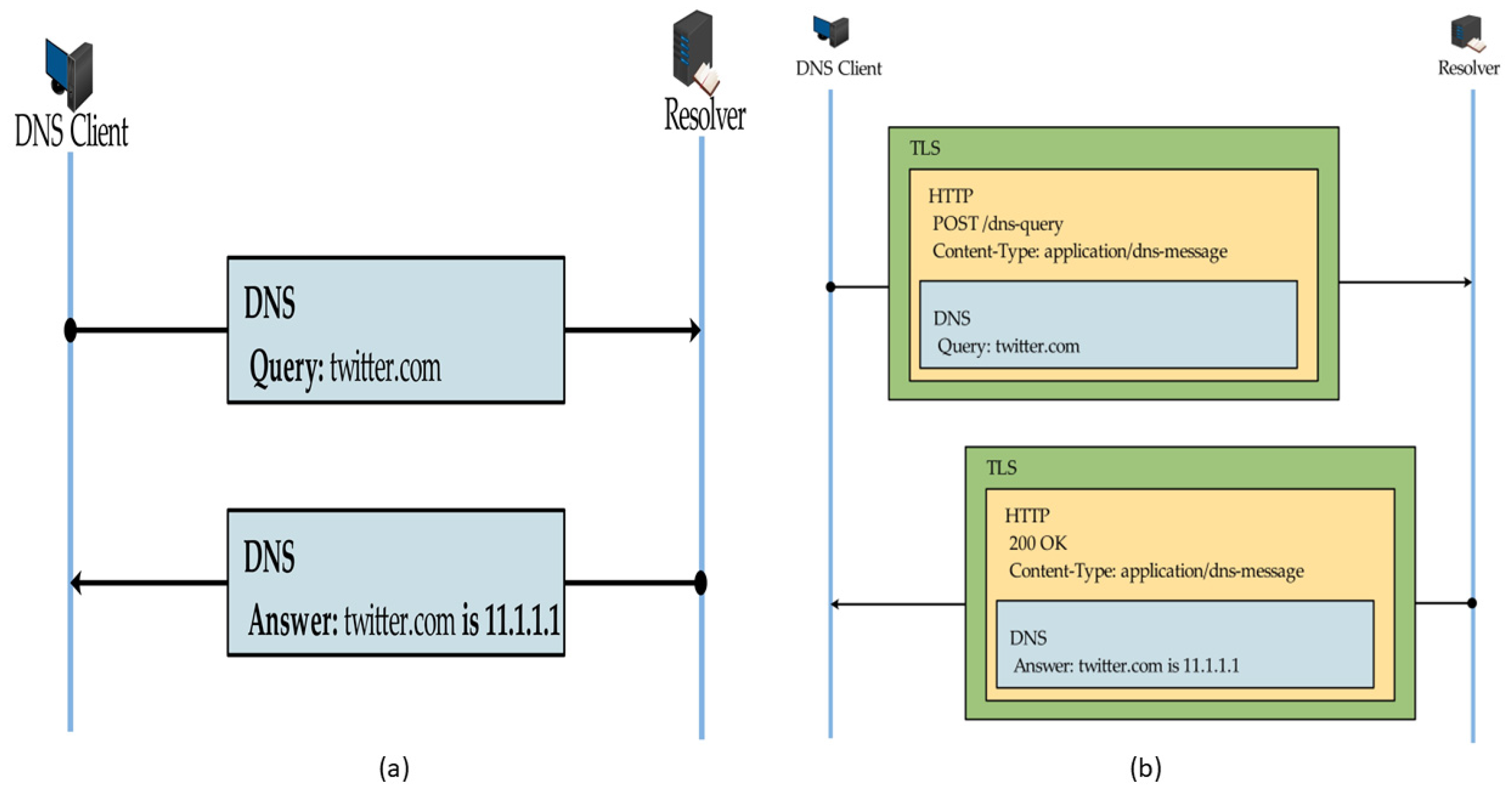
• Layer 1: The task of classifying HTTPS traffic into DNS-over-HTTPS (DoH) and normal web browsing activities (NonDoH). Dataset for this task is denoted as D.
• Layer 2: The task of characterizing DNS-over-HTTPS (DoH). Classifying DoH traffic into malicious or benign DoH. The dataset for this task is denoted as B. It is important to mention that we keep lower traffic samples of benign class in D as is and consider it to be the positive class for detection. Contrary to the commonly practiced methods of making malicious a minority, positive class, we deviate a little in order to prove otherwise.

3.2. Analytical Modeling of DoH Tunnels Using XTS

This section presents mathematical analysis of the proposed framework and its application to the detection of DNS-over-HTTPS tunnels in HTTPS traffic. We also explain the performance metrics used for highly imbalanced data.

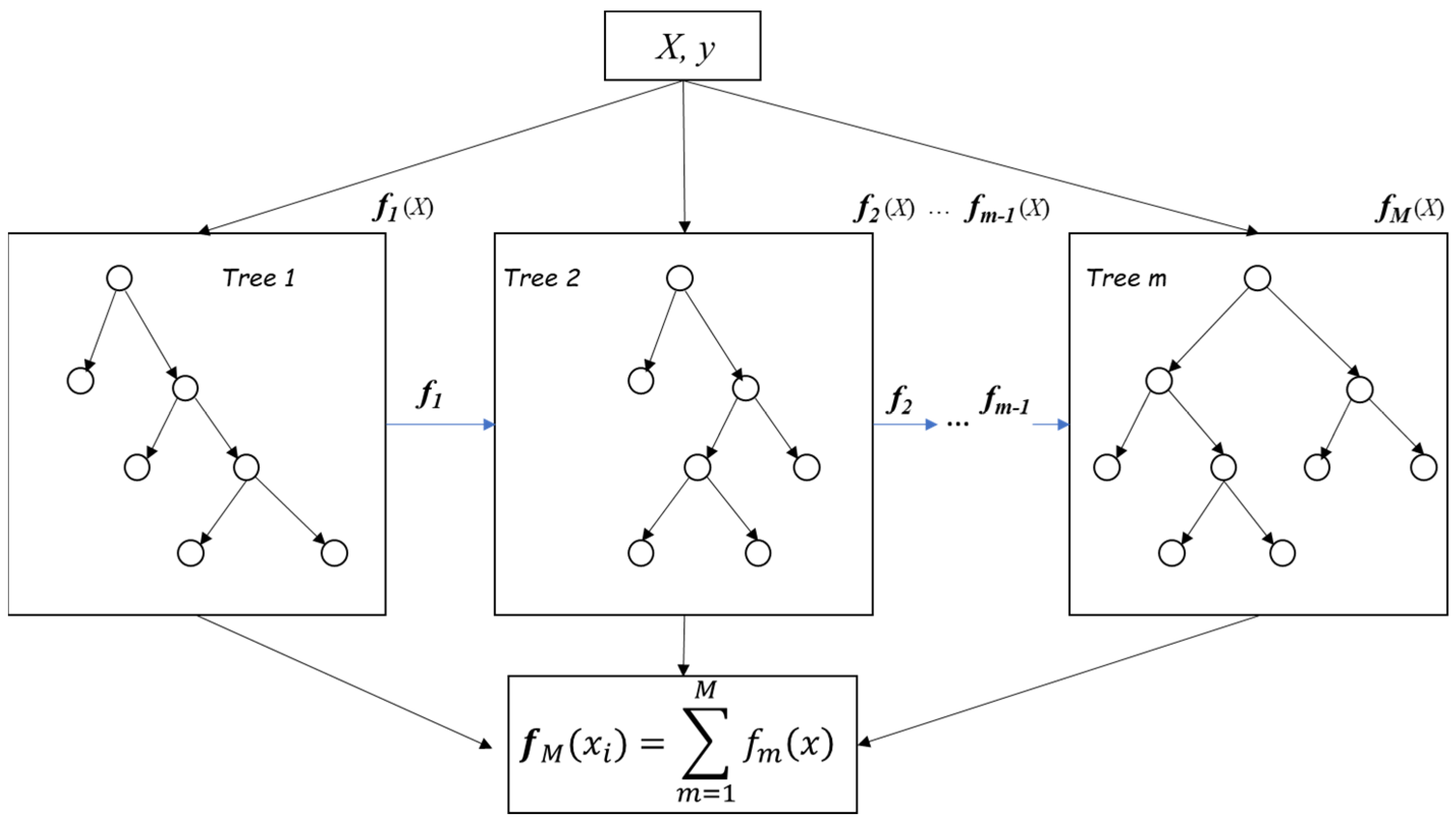
3.2.1. XGB Mathematical Abstract

Analytical modeling of HTTPS traffic flows using XTS framework involves using the XGBoost algorithm to learn a function that can predict the type of traffic flows in a network based on a set of input features. XGBoost uses classification decision trees called estimators as the base or weak learners. The final model output of a sample is a summation results of all the learners’ trained iteratively, as shown in Figure 4. Let $P=\left\{1, 2, 3, \dots M\right\}$ denote the set of weak learners, where $M$ is the total number of trees in the model. If $y_i$ is used to represent the true label DoH (1) or NonDoH (0), or Malicious (0), Benign (1) of a traffic flow $x_i$ in the dataset D or B respectively—in our case, then the predicted value $f_M(x_i)$ of the XGBoost model can be expressed in Equation (1) as:

$$f_M(x_i)={\displaystyle \sum _{m=1}^M{f}_m}(x_i), f\in F$$

(1)

where $F$ represents a set of all classification trees and $f_m(x_i)$ the individual base classifier’s prediction. The raw output or scores from each tree in XGBoost is referred to as the “raw prediction” and is denoted by z [62]. The predicted probability is then obtained by passing the raw prediction through the sigmoid function in Equation (2)

$$P(z)=\frac{1}{1+e^{-z}}$$

(2)

To minimize the objective function $obj(\theta )$, Equation (3) is computed as:

$$obj(\theta )=L(\theta )+\mathsf{\Omega }(\theta )$$

(3)

where $L(\theta )={\displaystyle {\sum }_{i=1}^{n}l(y_i, }{\widehat{y}}_i)$ is the loss function and $\mathsf{\Omega }(\theta )={\displaystyle {\sum }_{m=1}^M\mathsf{\Omega }(f_m})$ the regularization parameter that penalizes the complexity of the model. Since training happens in iteration process, the prediction value ${\widehat{y}}_i{}^{(t)}$ of an instance ith in iteration t, is expressed in Equation (4).

$${\widehat{y}}_i{}^{(t)}={\widehat{y}}_i{}^{(t-1)}+f_t(x_i)$$

(4)

Since the problem is a binary classification, we let the model use the predetermined loss function which is the cross entropy.in Equation (5).

$$L(y_i,{\widehat{y}}_i)=-[y_{i}log({\widehat{y}}_i)+(1-{\widehat{y}}_i)log(1-{\widehat{y}}_i)]$$

(5)

where $y$ is the true label (either 0 or 1) and $\widehat{y}$ is the predicted probability of the positive class (i.e., the output of the sigmoid function) $P\left(z\right)$ as shown in Equation (2). The loss is minimized when the predicted probabilities $\widehat{y}$ are as close as possible to the true labels $y$.

3.2.2. Dealing with Imbalance Data Using CX

Cost-Sensitive XGB assigns weights to training samples according to class proportions. This allows the algorithm to associate the cost of misclassification. Let $i$ be a predicted class and $j$ the actual class of an instance $x$. Let also $C\left(i, j\right)$ a function that computes the cost of predicting actual class $j$ as $i$, for instance, a model predict class DoH as nonDoH or Benign as Malicious, we assign heavy cost according to the class ratio. If we let $n$ be the total number of majority class, negative (0) and p the minority, positive class (1), the cost of misclassifying minority will be $n/p$ shows a matrix of how the algorithm assigns the cost for a binary classification. In Layer 1, we assign

The expected cost of classifying $x$ into class $i$ can be expressed in Equation (6).

$$C(i|x)={\displaystyle \sum _{j}P(j|x) C(j,i)}$$

(6)

In order to incorporate weighting and cost sensitivity into our XGBoost model for the classification of DoH and non-DoH traffic in Layer 1, as well as the classification of Benign and Malicious traffic in Layer 2, we adjusted the parameter C to assign different weights to each class as shown in Equation (6) and

Table 1. Cost matrix for binary classification.

	Predicted Positive	Predicted Negative
Actual Positive	C (1, 1) = 1	C (0, 1) = n/p
Actual Negative	C (1, 0) = 1	C (0, 0) = 1

. This allows us to consider the costs associated with misclassifying samples and tailor the model’s behavior accordingly.

3.2.3. Compared Models’ Computation Time Complexity

Let $D^{n\times m}$ be a dataset with n samples and m feature variables. Assume v is the number of support vectors, K the number of trees, d the depth of the tree and ${\Vert X\Vert }_0$ the number of non-missing entries in the training data.

Table 2. Computational time complexity of baseline models.

Model	TTT	TTD
LR	$O(n\times m)$	$O(m)$
SVM	$O(n^2)$	$O(v\times m)$
RF	$O(K\times n\times \log n\times m)$	$O(K\times m)$
XGB	$O(K\times d\times {\Vert X\Vert }_0+{\Vert X\Vert }_0\times \log n)$	$O(K\times d)$

shows the computational time complexity for each model that was used in this paper. To choose the best model, the time parameter was equally considered, with the assumption that, based on

Table 3. Traffic flows features.

Category	Feature Name
Flow Direction	F1: Source IP, F2: Destination IP, F3: Source Port, F4: Destination Port.
Packet Bytes	F5: Duration, F6: Number of flow bytes sent, F7: Rate of flow bytes sent, F8: Number of flow bytes received, F9: Rates of flow bytes received.
Packet Length	F10: Mean, F11: Median, F12: Mode, F13: Variance, F14: Standard deviation, F15: Coefficient of variation, F16: Skew from median, F17: Skew from mode.
Packet Time	F18: Mean, F19: Median, F20: Mode, F21: Variance, F22: Standard Deviation, F23: Coefficient of variation, F24: Skew from median, F25: Skew from mode
Request/response time difference	F26: Mean, F27: Median, F28: Mode, F29: Variance, F30: Standard Deviation, F31: Coefficient of variation, F32: Skew from median, F33: Skew from mode.

, if $M$ is a vector space of dataset features, reducing $M$ to a very significant number $S\subseteq M$ will result in low-dimensional representation data, thus presumably reducing computational cost (time and space). In our experiment, we performed empirical tests while observing the model’s prediction performance. Overfitting was observed diligently.

3.2.4. Speed Optimization Using gCX

The XGB model provides many parameters and methods commonly used to minimize computational cost, such as reducing the number of trees, column sampling, pruning a tree, among others. Finding the optimum parameters require trial and error process, which takes more time. However, with the pervasive use of GPU-based processors in today’s laptops, many researchers have not realized the great speed benefits of running a GPU-based XGB model. This paper demonstrates the difference between running a GPU and CPU-based XGB models as a simple but effective means of minimizing computational cost.

According to Tianqi et al. [62,63], there are 4 tree methods, namely exact, approx, hist and gpu_hist used as split finding methods; they have a great impact on XGB computational time. exact tree method is slower in performance by $O(K\times d {\Vert X\Vert }_0 + {\Vert X\Vert }_0 \times logn)$ and not scalable. approx tree method makes the algorithm faster than the previous by $O(K\times d\times \parallel X{\parallel }_0+\parallel X{\parallel }_{ 0}\times logB)$, where B is the maximum number of rows in each block. Unlike approx., which generates a new set of bins for each iteration, the hist method reuses the bins over multiple iterations. It is a faster tree construction method on CPU computers. Although the hist method was faster than all its predecessors, Mitchell et al. [64] developed a CUDA-capable GPU method to construct a tree algorithm, namely the gpu_hist method. We only set the following parameters in our experiment, namely, generic XGB speedup to ($11 \mathrm{times}, 1.08 \mathrm{times}$) in layer 1, and ($5 \mathrm{times}, 1.14 \mathrm{times}$) in layer 2 for $\mathrm{TTT}$ and $\mathrm{TTD}$, respectively. This model is represented as gCX in the framework.

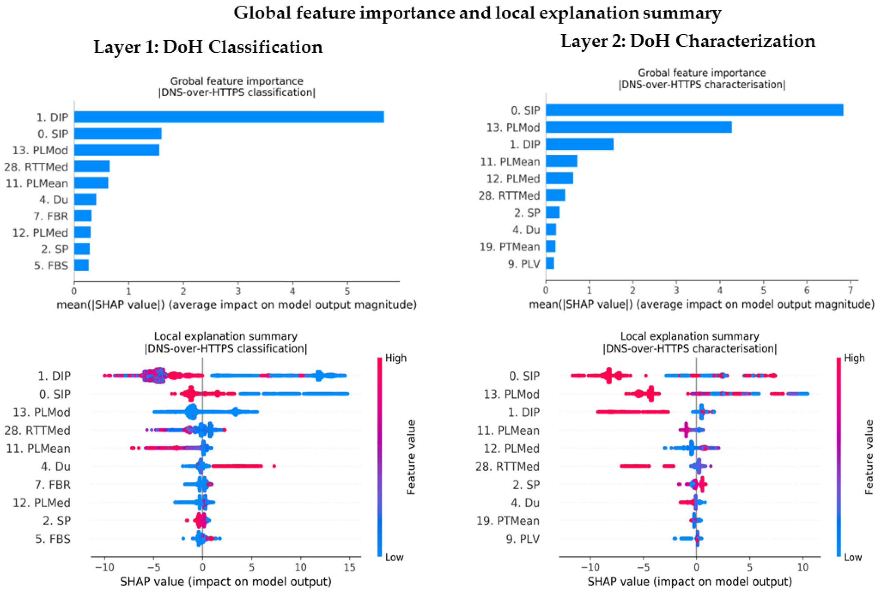
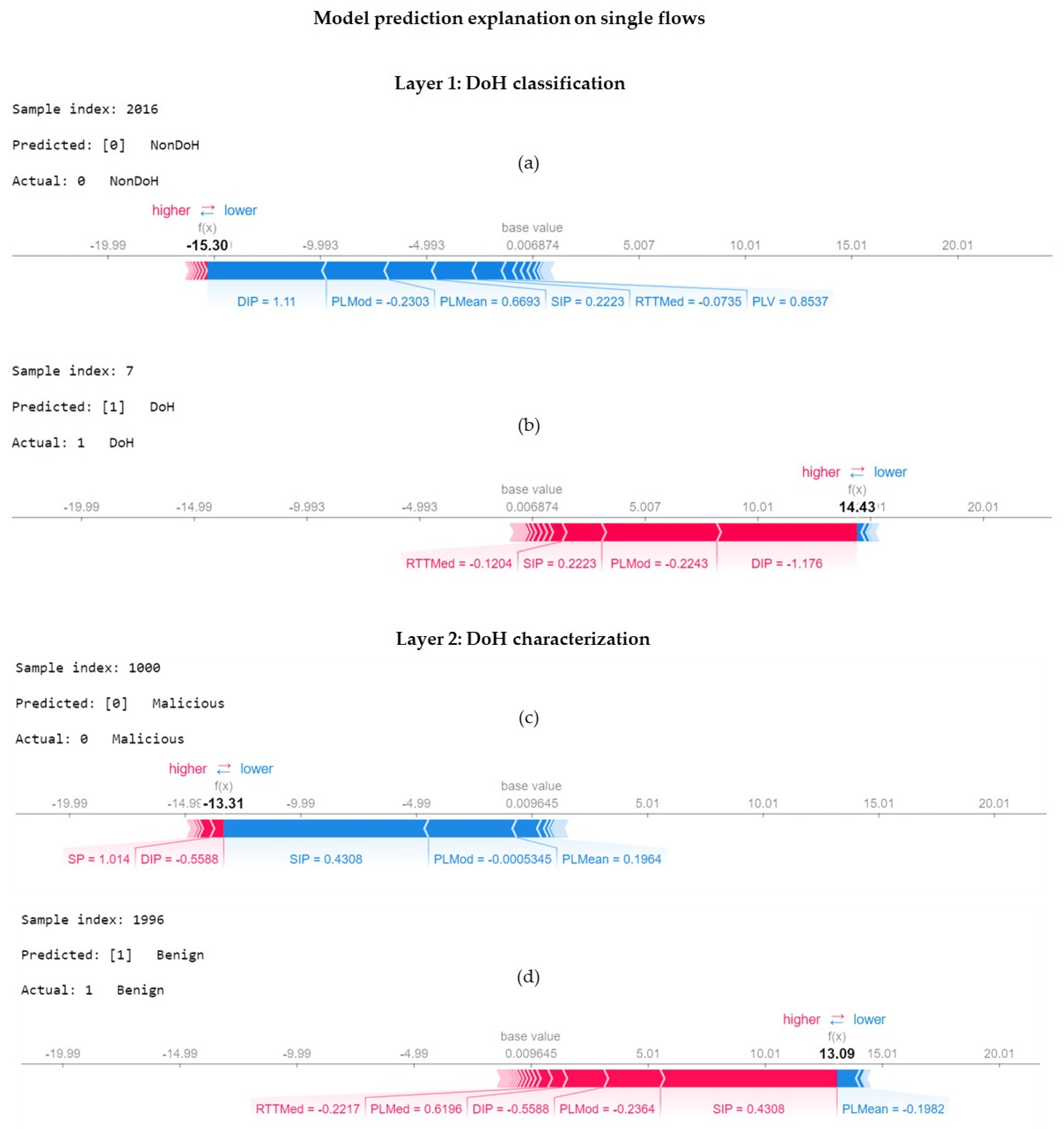
3.2.5. Feature Importance Modeling and Analysis

In this section, we employ the Tree Explainer method to interpret the prediction output of our gCX model and learn the importance of features in predicting the samples in our datasets, or in a specific sample $x_i$. The Tree Explainer is a variation of SHAP (SHapley Additive exPlanations) kernels, which are based on the concept of SHAP values.

SHAP values were introduced by Lundberg and Lee in 2017 [65], drawing inspiration from the coalitional game theory developed by Lloyd Shapley [66]. These values provide a principled approach to fairly distribute the contributions of features towards the model’s output, ensuring interpretability and an understanding of feature importance.

We choose to utilize the Tree Explainer method instead of the kernel explainer due to its computational efficiency. The Tree Explainer leverages the tree-based structure of the XGB model to approximate the SHAP values, resulting in faster computation times while still providing reliable interpretations of feature importance [67].

To model the feature importance using SHAP values, let M denote a set of all input features of a dataset D or B and gCX indicate the previously optimized XGB classifier (that maps input feature vector $x\in {ℝ}^{\left|N\right|}$ to an output $f\left(x\right)\in \left[0, 1\right]$ for DoH tunnels classification. SHAP values present the only single solution to “fairly” spread the features contributions towards $f\left(x\right)$ and satisfies three desirable properties: local accuracy, missingness, and consistency [60,61].

Let $f_x\left(s\right)$ denote the model’s output constrained to the feature subset $S\cup M$. Based on the classical Shapley values [original], SHAP values are generally computed as follows:

$$\varnothing i={\displaystyle \sum _{S\subseteq M\backslash \left\{i\right\}}\frac{\left|S\right|!\left(M-\left|S\right|-1\right)!}{M!}\left[fx\left(S\cup \left\{i\right\}\right)-fx\left(S\right)\right]}$$

(7)

where $f_x\left(S\cup \left\{i\right\}\right)$ is the model’s output of the instance $x$ constrained to the feature set $S\cup M,$ excluding the ith feature. SHAP was designed as an model-agnostic explainer $g$ to mimic the process that the original model $f$ used to predict a specific prediction so that $f\left(x_i\right)\approx g\left(x_i\right).$ To compute the contribution of a feature $j$, referred to as $I_j$, where $j\in M$ feature set, its mean absolute SHAP values across the dataset is calculated as follows:

$$I_j=\frac{1}{n}{\displaystyle \sum _{i=1}^n\left|{\varnothing }_j^{\left(i\right)}\right|}$$

(8)

TreeSHAP: It is a variant of SHAP Kernel method. Kernel method is model-agnostic, whereas TreeSHAP was designed specifically for tree-based models such as decision tree, random forest and gradient boosting models. Unlike Kernel SHAP, Tree SHAP computes SHAP values in polynomial, rather than exponential, time to reduce the computational time by $\mathrm{O}\left({\mathrm{TLD}}^2\right)$ from of $\mathrm{O}\left(\mathrm{TL}{2}^{\mathrm{M}}\right)$, which makes it faster than its counterpart; T is the number of trees; L is the maximum number of leaves in any tree; and D is the maximum depth of any tree. Due to the additive nature of SHAP, the output SHAP value on an ensemble model is a weighted average of the SHAP values of the individual tree.

SHAP values plots: a feature SHAP value can be calculated for all or some samples in the dataset. The SHAP library provides plots to summarize features at the local and global view. In this paper, three plots (force plot, feature importance plot and the summary plot) were chosen to present the results.

The force plot [53,65,65] shows how each feature value pushes to increase the baseline towards the model’s output value.

A baseline or base value on the plot is the value that would be predicted if the features contributions were unknown to the current model output $f\left(x\right)$. In other words, it is the mean prediction of the model’s explainer on the passed dataset. Equation (9) shows the formula used to compute the baseline value.

$$\overline{\widehat{y}}=\frac{1}{n}{\displaystyle \sum _{i=1}^n\widehat{y}}$$

(9)

In the force plot as shown in Figure 5, features are stacked in colored (red/blue) arrows or bars according to their SHAP values $(\varnothing )$. Red bars, pushing towards right, means that, the corresponding feature’s original value pushes the model to the higher output $f\left(x\right)$ from the base value calculated in Equation (10). By higher output, it means positive class, in a binary problem. On another hand, the blue bars, pushing towards left, means that, the corresponding feature’s original value pushes the model to the lower output $f\left(x\right)$ negative class (0) from the base value.

The magnitude of the bar indicates the degree of influence, measured in SHAP values, which a feature has on the model’s output. For a binary problem, the positive model output, which could be the probabilities or log odds, indicates a positive (1) prediction. Conversely, a negative output means a negative class (0) prediction. It is to be noted that Tree Explainer library in the Scikit-learn library as of the writing of this paper, allows the model output to be ‘raw’, indicating the score values of the underlying tree model before the sigmoid function is used to compute probabilities. They are real-valued numbers in the form of log-odds. The positive numbers represent the high confidence of the model to predict a sample $x_i$ as a positive class (1). To achieve this, we set the link function to logit for the model to transform the log-odds back into probabilities, something which can be achieved separately using the sigmoid function shown in Equation (2). This is due to the known property of inversibility between logit/log-odds function and sigmoid.

A feature importance plot displays sorted global SHAP values of the features on $\left(x,y\right)$ axis, where $x$ indicates a scale of SHAP values ranging from (low to high) and $y$ the features from MSF (top) to LSF (bottom).

The summary plot shows the relationship between the values of the feature and their impact on the prediction. The SHAP values of individual samples are plotted onto a 2D graph as dots across the $x$ axis against their corresponding features to a form SHAP value distribution (a bee-like swarm), as seen in Figure 6. Each dot (SHAP value) is presented in color (red, blue) to indicate the magnitude of the original feature value. The intensity of the colors on the color bar (right of the plot) indicates the degree of the original feature’s values across the entire column in the dataset. A strong red (top of the bar) means a higher value and a strong blue (bottom of the bar) means a lower value. To determine whether a value is high or low, it is compared to its column’s average value. If the value of the feature is greater than its average, its corresponding SHAP value is colored with red. In the inverse situation, it is colored blue.

3.2.6. Low-Dimensional Representation Using SFE

A Sequential Forward Evaluation algorithm is developed in this paper to evaluate how the gCX model performs on features subsets. Algorithm 1 shows how gCX is evaluated on each subset. $S_M$ is a set of integer numbers $(u_1, u_2, u_3, \dots , u_m)$. They are the indices of features in $S_M$. The process starts by initializing a variable $R_s$ to hold a set of feature indices. The algorithm employed in this approach does not rely on complex mathematical constructs, such as permutation or shuffling. Instead, it adopts a simple feed-forward design principle. Despite its simplicity, this algorithm enables us to sequentially evaluate the model’s performance and gain valuable insights into the importance of different features in determining a model’s output.

By creating subsets of features and evaluating the model using these subsets, we are able to achieve high prediction scores while keeping the dimensionality relatively low. This approach allows us to effectively analyze and understand the contribution of individual features to the model’s output. It also addresses the challenges posed by high dimensionality in the dataset, which is an important consideration in many real-world applications. For each iteration, the model operates on the next newly formed $S_i$. This allows the model to access all samples of the dataset by using the selected features to study the contribution of the feature subsets without changing their contribution order.

For each iteration, error rate or loss and aucpr curves are displayed to monitor the model’s learning process. $TTT$ and $TTD$ are each recorded in a variable set to keep track of computational time by subset. Additionally, other evaluation metrics are recorded for comparison.

Algorithm 1: Sequential Forward Evaluation.
	Input: A list of $m$ top 10 selected features from the main feature set $M$
	Output: Computational time ($TTT, TTD)$, evaluation metrics ($P, R, F1, AUCPR, loss)$ for all subsets
1	Require: $S_{M }\leftarrow \left[u_1, u_2, u_3, \dots , u_m\right];u\in {\mathbb{Z}}^{+}; \mathrm{S} \subseteq \mathrm{M}$ Create a subset $S_{M }$ of selected top features $m$ from original feature set $M$
2	Initialize: $R_s\leftarrow \varnothing ; t_{train}\leftarrow \varnothing ; t_{pred}\leftarrow \varnothing ;R_s\subseteq S_{M }$// initialize features index and time sets to null
3	Procedure ($X_{train}; X_{val}; X_{test}; y_{train}; y_{val}; y_{test}$)
4		for all $u \in S_{M }$ do // create a subset for each iteration
5			$R_s\leftarrow R_s\cup \left\{u_i\right\}$// add one feature to create a new subset
6			$t_{0 }\leftarrow time.time()$ // time before training and validation
7			$cfr \leftarrow f\left(X_{train}\left[:, R_s\right], y_{train}, [\left(X_{train}\left[:, R_s\right], y_{train}\right), (X_{val}\left[:, R_s\right], y_{val}\right)])$// train the model
8			$t_{1 }\leftarrow time.time$ // time after training and validation
9			$t_{t }\leftarrow$ $t_{1 }-t_0$// Time-to-Train (TTT) including validation time
10			append $t_{t }$ to $t_{train }$// add TTT of a subset to training time set
11			$t_0^{\prime } \leftarrow time.time()$ //time before testing
12			$y \leftarrow cfr\left(X_{test}\left[:, R_s\right]\right)$ //test the model
13			$t_1^{\prime } \leftarrow time.time()$ //time after testing
14			$t_{d }\leftarrow$ $t_1^{\prime } -t_0^{\prime }$//Time-to-Detect (TTD)
15			append $t_{d }$ to $t_{test }$// add TTD of a subset to prediction time set
16			record $log$
17			call plot functions ($y_{test}, y_{pred}$)
18		end for
20	end procedure

3.2.7. Model Performance Metrics

Throughout this paper, the model’s performance evaluation is measured in two dimensions: model’s prediction performance using (precision, recall, F1-Score, AUCPR, confusion matrix) and computational time (time to train and time to detect). Prediction performance metrics: precision (P), recall (R), F1-Score (F1) and AUCPR are the ML metrics suitable for application to problems with highly imbalanced or skewed data.

DoH samples in layer 1 represent the positive class (minority), while NonDoH samples represent the negative class (majority). Benign flows in layer 2 represent the positive class (minority) and malicious flows represent the negative class (majority). For highly imbalanced data, the model tends to be biased towards the majority class, where huge number of actual positive samples are predicted as negative (FN). In rare cases, the actual negative samples may be predicted as positive (FP). Hence, in the most cases as in our case of security incident monitoring, the success of the model is measured on how it correctly predicts the positive class (low FN). Since the benign class is the minority/positive class in our case, we pay attention to how the model detects this class rather than the malicious class, as described in Section 3.1.

To achieve this goal, a confusion matrix for binary classification is created to further help in calculating other metrics.

• Precision: Precision metric shows, from all the instances that the model predicted as belonging to the positive class (TP + FP), the percentage of those which were actually true positive (TP). In this paper, it refers to how many DoH samples were predicted correctly out of all predicted as DoH and/or how many benign samples were predicted correctly out of all predicted as benign, in layer 1 and layer 2, respectively.

  $$P=\frac{TP}{TP+FP}$$

  (10)
• Recall: Recall metric shows, from all the instances of positive class (TP + FN), the percentage of those which the model predicted correctly. In this paper, it refers to how many DoH or Benign flows were predicted correctly in layer 1 or 2 respectively.

  $$R=\frac{TP}{TP+FN}$$

  (11)
• F1-Score: F1-Score measures the overall average of both Precision and Recall.

  $$\mathrm{F}1=2\frac{P\ast R}{P+R}$$

  (12)
• AUCPR: Area Under the (Precision-Recall) Curve also known as Average precision (AP), shows a relationship between the Recall and Precision on a scale between 0 and 1. Equation (13), shows how to compute AP, where $R_n$ and $P_n$ mean the recall and precision at the ith threshold. Unlike AUC-ROC curves which considers the balance between positive and negative classes, AUCPR/AP focuses on how correctly the positive (minority) class is predicted [68]

  $$AP={\displaystyle \sum _n(R_n}-R_{n-1})P_n$$

  (13)

If these metrics are used by the IDS implementing this model, FP may be noisy warnings but less dangerous than FN in layer 1, which is opposite in layer 2. However, security guidelines are defined by the company rules. In this paper both metrics are equally important, though much focus is put on the minority class to avoid the errors which may be caused by the imbalance and skewness of the dataset [24].

3.3. Proposed Application Domain

At the edge AI network, IoT or other devices may be compromised by a remote C2 implementing DoH tunneling attacks, as shown in Figure 7. A rule-based firewall may not be able to detect intrusion due to similarity with normal HTTPS traffic. For a supervised task of this kind, $XTS$ would be recommended, among other solutions. The idea of this framework was inspired by the recent research buzz surrounding the newly envisioned 6G technology and intelligent multimedia [5,6,7,8].

This new technology, as was mentioned in Section 1, anticipate enormous amount of heterogeneous data due to the sparsity of data and their imbalanced nature; $TTT$ and $TTD$ are among the concerned parameters. Information security is also among areas that will undoubtedly be affected. Therefore, an approach is needed that reduces data dimensionality and enables small devices to collect only a small number of variables and improve model interpretability. The solution should not only help us to minimize computation cost but also should assist users to understand consistency and individualized model output decisions. Additionally, it may need to minimize the attack surface due to reduced user features. This framework would serve as an abstract view of how security devices such as IDS or SIEM at the edge network would be optimized to report more accurate and understandable results, while reducing computation costs in a growing ecosystem of faster data.

4. Materials and Methods

This study is a computer experimental-based design. This section explains the experimental procedures used to empirically evaluate the design of the XTS framework redescribed in the previous sections.

4.1. Dataset Description

The dataset namely CIRA-CIC-DoHBrw-2020, used to evaluate the proposed method, was created by the Canadian Institute for Cybersecurity (CIC) project, which was funded by Canadian Internet Registration Authority (CIRA). It was made publicly available by [69]. The authors of this dataset conducted DNS-over-HTTPS tunneling attack using proof-of-concepts tools in a lab-controlled environment. They followed a two-layered architecture: in layer 1, they classified HTTPS traffic into DNS-over-HTPPS (DoH) and normal HTTPS web browsing activities (NonDoH). In layer 2, DoH traffic flows were characterized into malicious DoH and benign DoH.

The data were captured in two phases: In the first phase of data capturing, web browsers (Google Chrome and Mozilla Firefox) were configured to send DNS requests to the public DoH resolvers (AdGuard, Cloudflare, Google DNS, and Quad9) through a local DoH proxy server. The flow samples were captured between the proxy server and the public DoH server to include both (benign DoH) and normal HTTPS browsing activities (NonDoH). In the second phase, three DoH-based C2 tunnelling tools (namely, Iodine [70], DNS2TCP [71], and DNScat2 [72]) were used to communicate with malicious C2 servers on the Internet. To make sure that only malicious DoH traffic (malicious DoH) was captured, other browsing activities were prevented. All traffic were captured as bi-directional traffic (where requests and responses are combined in one flow) and saved in PCAP files. A new custom application namely DOHLyser [73] was developed to extract flow-based statistical and timeseries features and saved as CSV files.

4.2. Experimental Setup

4.2.1. Overview

The experimental setup in this study aimed to rigorously evaluate the performance of the proposed XTS framework in DNS/DoH tunnels detection as described in Figure 8. The selection and preparation of suitable datasets, along with careful parameter tuning and model comparisons, were conducted to ensure the obtention of robust and meaningful results.

The datasets used in this experiment consisted of a diverse range of network traffic, including normal HTTPS, benign, and malicious traffic. These datasets were obtained from a publicly available repository, ensuring the availability of real-world and representative samples. To ensure that the datasets were appropriately processed, several steps were taken. IP addresses were converted into numerical integer values to facilitate analysis and modeling. Feature scaling, imputation of missing variables, and the label encoding of target classes were performed to ensure compatibility with the chosen machine learning algorithms. A comprehensive comparison was conducted among five well-known machine learning models, excluding deep learning models. In this comparison, default parameter settings were used for all models, except for models that could be transformed into cost-sensitive models. Models not designed with this feature, such as Bayes models, were excluded from initial consideration.

Standard XGB was hyper-parameterized, taking into account cost sensitivity and speed optimization. GPU acceleration was utilized to leverage computational power for use in efficient training and testing. To gain insights into the model’s decision-making process, the SHAP Tree Explainer was applied to provide interpretable explanations. Three types of SHAP plots were generated: a global SHAP summary plot, local explanations, and individualized sample explanations. These visualizations helped use to identify the most influential features and understand how they contributed to the model’s predictions. Additionally, feature subset evaluation was conducted to assess the impact of different feature combinations on the model’s performance. A sequential algorithm was employed to create subsets of increasing size, and training and testing were performed for each subset. This analysis allowed for a deeper understanding of the importance and relevance of specific features in the DNS/DoH tunnels detection task.

The experimental setup was designed to be rigorous, scientifically valid, and comprehensive. By leveraging appropriate datasets, conducting model comparisons, hyperparameter tuning, and utilizing explainability techniques, the XTS framework demonstrated its effectiveness in addressing the DNS/DoH tunnel detection problem. The subsequent sections will present the results and discuss their implications in detail.

We trained the newly hyper-parameterized XGBoost on full features datasets, split divided into three distinct subsets: training, validation, and testing, with sizes of 60%, 20%, and 20%, respectively. The experiments were conducted on a Lenovo laptop, which featured an Intel i7-9750H CPU with 6 cores clocked at 2.6 GHz, a Pascal GTX 1050 GPU with 2 GB of memory, and 8 GB of RAM. Important parameters were set as follows: objective function = ‘binary:logistic’, booster = ‘gbtree’, n_estimators = 100, scale_pos_weight = majority_class/minority_class, tree_method = ‘gpu_hist’, eval_metric = [‘logloss’, ‘aucpr’]. To track the results of separate datasets, an instance for each dataset was created. There were, on average, 20 epochs on average and 7-fold CV.

The loss/AUCPR log results were collected to plot loss and AUCPR values. A trained model instance was fitted in the SHAP Tree Explainer for interpretation. Three SHAP plots were created—global shap summary plot, local explanations and individualized sample explanations. We selected the top 10 most significant features and created 10 subsets sequentially using written Algorithm 1. These were recorded for each training and testing time, along with prediction scores, each time a new subset was created. Finally, the different results were compared.

4.2.2. Data Engineering

To begin with, the source and destination features, represented as string objects, were converted into numeric whole numbers. We performed this with the intuition that the model could learn some insights from the numerical representation of the source and destination. Another study considered this before and argued that the model would present its decision in numerical format. For us, these features were crucial in our working hypothesis. Feature scaling using standardization Equation (14) was applied to all integer features to reduce their magnitudes, thus increasing the chance to prevent model’s overfitting and speed up its convergence.

$$z=\frac{x-\mu }{\sigma }$$

(14)

A new score $z$ or standard is computed from $\mu$ (the mean) and $\sigma$ (the standard deviation from the mean). This technique scales the feature values in the range $\left[-1, 1\right]$, so that they will have properties of the standard normal distribution with the mean $\mu =0$ and the standard deviation $\sigma =1$. Since this is a binary classification problem, a vector $y$ is encoded and assumed to represent the target variable such that, ${\mathrm{y}}_1=[0, 1]$ represents the target variable in layer 1, where 0 means NonDoH and 1 is the DoH class. On another hand, ${\mathrm{y}}_2=[0, 1]$ represents the target variable in layer 2, where 0 means Malicious and 1 is the Benign class.

Both datasets D and B exhibit a high degree of class imbalance, as revealed by the samples per layer presented in Figure 9.

Based on the numbers in

Table 4. Sample sizes per class.

Layer 1: Classification of HTTPS Traffics
Class	Sample size
NonDoH	897,493
DoH	269,643
Layer 2: DoH Characterization
Benign DoH	19,807
Malicious DoH	249,836

, the graphical distribution of classes depicted in Figure 9, specifically, Figure 9a, displays a class ratio of 8:2, while Figure 9b exhibits a more imbalanced ratio of 9:1. Moreover, both datasets contain 16,056 missing values each, and therefore, imputation was performed on the relevant variables by filling the missing values with the column mean, as per Equation (15).

$$\widehat{x}=\frac{1}{n}{\displaystyle \sum _{i=1}^n{x}_i}$$

(15)

4.2.3. Model Selection

Based on a comparative analysis with other popular machine learning models, including logistic regression (LR), support vector machine (SVM), and random forest (RF), we found that XGB outperforms other models on the selected datasets. Our selection of XGB was based on its empirical performance in terms of accuracy and computational efficiency. Additionally, our choice was motivated by its popularity and its widespread use in the machine learning research community [74]. All the models were trained with default parameters, with their respective cost-sensitive parameters being set as indicated in Section 3.2.2.

The comparison of both dataset D and B indicates that LR exhibits faster training and detection times compared to other models, albeit with the lowest F1-score, Figure 10. SVM, on the other hand, achieves excellent F1-score but at the expense of being the slowest model. RF and XGB demonstrate outstanding F1-scores, with XGB outperforming RF in terms of training latency and detection speed. Specifically, RF’s training latency is nearly 5 times that of XGB, while its detection speed is approximately 20 times slower than XGB. The selection of XGB was based on its higher prediction performance, lower training latency, and faster detection speed. The elimination criteria were primarily based on prediction performance and computational time. Other factors, such as missing value handling and scalability, were also taken into account, especially in cases where models had similar results, as shown by RF and XGB in Section 5.

5. Results and Discussion

The gCX model demonstrated unrivaled performance compared to other models in the experiments. It outperformed the baseline models in terms of predictive accuracy, precision, recall, and F1-score as shown in Figure 10. The utilization of weighted parameters and the incorporation of SHAP values for feature importance analysis played a role in achieving this superior performance. The gCX model’s ability to handle class imbalance and its effective utilization of the underlying structure in the data contributed to its exceptional results. These findings highlight the effectiveness of the gCX model in tackling the challenges posed by the DoH tunnels dataset and its potential to make accurate and reliable predictions in the context of highly imbalanced-binary classification tasks.

5.1. Prediction vs. Computational Time

This section of the findings addresses the concern of overfitting that may arise from the results presented in Figure 11 and Figure 12. While the possibility of overfitting is acknowledged, we have not found substantial empirical evidence to support this assumption. Several reasons contribute to this perspective. Firstly, gCX, our chosen model, is optimized using the best parameters specifically tailored for the problem under investigation, as outlined in Section 4. This optimization process enhances the model’s performance and reduces the likelihood of overfitting. Secondly, the models employed in this research have been widely recognized as exceptional within the research community. Their effectiveness and reliability have been extensively demonstrated in various studies, providing further confidence in their robustness. Thirdly, the evaluation metrics used, such as the confusion matrix and log-based measures (log loss, AUC–PR), are well-established and trustworthy for use in assessing imbalanced models. These metrics offer reliable insights into the model’s performance and its ability to handle imbalanced datasets. Fourthly, the dataset used in this study is relatively large, providing a sufficient number of samples for training and evaluation. Adequate sample size plays a crucial role in mitigating the risk of overfitting, and our dataset meets this requirement. Furthermore, we employed scientifically accepted methodologies to split the data and applied 7-fold cross validation, a widely recognized unbiased estimation method used by researchers in various machine leaning domains. For instance, K. Nkurikiyeyezu [75] provided convincing arguments on the same issue. Additionally, we conducted evaluations on subsets of the most significant features, Figure 11, further strengthening the reliability and generalizability of our findings. Based on these arguments, we are inclined to reject the notion that the model’s exceptional performance on our labeled datasets is solely due to overfitting. However, we acknowledge the need for further research and exploration to deepen our understanding of both the data and the model’s capabilities. By conducting additional investigations, we aim to gain more insights and validate the model’s performance in diverse scenarios and datasets.

As stated, starting this section, we can observe in Figure 12a that when the model is trained only with one feature (S1) in the S_M list—Destination IP—according to Figure 13, it successfully recognizes all instances of DoH traffic and avoids false negatives, ensuring that no DoH traffic goes undetected. However, the relatively high number of false positives indicates that the model is also misclassifying a significant amount of non-DoH traffic as DoH. It is also the case in (b), where the model successfully detected many instances of benign DoH traffic, missing (FN) only around 21% (663) but misclassifying more than 14% (7123) of malicious traffic (FP). Expectedly, when the model is trained on the combined destination and source IP (S2) features (a), FP is reduced towards 0 (only 30 out of 179, 549), which is also the case in (b). These results confirm our hypothesis that C2 traffic is likely to be detected based only on unique connections at the IP level (the source and destination IPs) and probably with packet length statistical features such as packet length mode, mean, or median. The packet length effect was shown in (a), where 0 FN and FP are achieved only with 3 features (S3)—the first three most important features according to Figure 13, Layer 2. Consequently, based on the above empirical evidence, we can objectively reject the assumption of overfitting for the gCX model.

5.2. Feature Importance

In Figure 13, it is observed that at the global view, the model is likely to classify HTTPS traffic based mostly on three features, destination IP (DIP), packet length mode (PLMod) and source IP (SIP). Local explanation provides further insights about these features. For instance, there is a clear cut showing that, as the values of the feature samples become higher (which specifies that their values are higher than their respective column mean) in detecting benign flows (lower right), the model grows certain about the malicious class (negative SHAP values). The same is observed in Figure 14 (lower right) for sample 1996. It shows that, values of DIP, SIP and PLMod push the model to predict positive class (Benign), which is also the case for sample 7 (lower left).

Although this might not be generalized to the real-world scenario, where IP addresses vary significantly, we observed in our study that IP address numbers assigned to DoH tunnel computers are larger than those of benign traffic. In this case, we may assert that may the model was correct in predicting malicious traffic. There is supporting evidence behind the model basing its prediction on both flow connection and packet length size features in traffic flow analysis using statistical modeling.

The bold numbers on the SHAP values line in Figure 14 show the summation of all feature contributions and the expected value of the model towards the prediction of an individual sample [52] and are represented as log-odds. The color shows the magnitude of the feature values—not the SHAP values, where red indicates that the values of particular features were higher than the mean of their respective columns in the dataset and blue indicates otherwise [51]. We can observe in Figure 14a,c that whenever the values of the features are lower than their respective mean (blue), they push the model, gCX, to predict negative classes (non-DoH or malicious) following the order of feature contributions, contrary to the observation seen in (c) and (d), where values higher (red) than their mean push the model to predict positive classes (DoH or benign) following the order of feature contributions. It is important to note that there is not always an exact match between a single sample (Figure 14) and the overall local explanations (Figure 13, second row).

5.3. Comparison and Discussion

This research includes a comprehensive comparison of the proposed XTS model with other studies in the literature that utilized the same dataset and employed similar computational time measurements. It is unfortunate to note that many researchers did not provide extensive details of their experimental setup. However, even with these limitations, our findings highlight the superior performance of XTS as shown in

Table 5. Comparison of the proposed framework (XTS) with related studies in the literature. *—the best performing methods before XTS; TTT—training time; TTD—testing time; (-)— indicates that we could not find these values in the mentioned papers. Where there were two values in the cell, it means the authors did not use two-layered architecture, i.e., Layer 1 and Layer 2, respectively. Because all the models have demonstrated exceptionally high prediction scores, we consider the best performers as overall but focus on TTT(s) and TTT(s). For example, ref. [53] shows missing F1, P and R in their methods; however, they demonstrate TTT and TTD earlier than others. The presence of (-) in the Features column means that authors did not conduct the low-dimensionality representation process.

Methods	AUCPR/ROC	F1	P	R	TTT(s)	TTD(s)	Features
Layer 1: Classification of HTTPS into DoH and NonDoH
LSTM [76]	-	99.3	99.3	99.3	-	0.574	3
LGBM [36] *	99.9	99.9	99.9	99.9	87	0.08	27
Decision tree, random forest [58] *	[98, 1]	-	-	-	[11.9,31.7]	[0.041,0.216]	-
XTS (proposed framework)	99.99	99.96	99.94	99.99	1.8	0.07	3
Layer 2: DoH characterization into Malicious DoH and Benign DoH
LSTM [76]	-	99.1	99.1	99.1	-	0.502	5
LGBM [36] *	99.9	99.9	99.9	99.9	40	0.08	27
ABG-VAE [77]	-	99.4	99.2	99.6	12.24	1.1	-
Decision tree, random forest [58] *	[1, 1]	-	-	-	[72.24,118.78]	[0.098,0.586]	-
XTS (proposed framework)	1	1	1	1	0.7	0.016	5

.

Our research emphasizes the unique strengths of the XTS model, including its exceptional computational efficiency and prediction performance. By significantly outperforming previous models in terms of computational speed and maintaining or surpassing their detection capabilities, XTS establishes itself as the best-performing solution for DNS/DoH tunnels detection within the compared space. We welcome other researchers to make further improvements to our work.

In summary, the comparison of XTS with other research using the same dataset and computational time measurements reveals its significant advantages. XTS outperforms previous models in terms of computational efficiency, being substantially faster in both TTT, TTD and reduced features. Additionally, XTS demonstrates equal or superior prediction performance compared to the best performing models in the literature. Moreover, it was the only model found to have combined bridged or at least touched different research problems shown in Figure 2, all together. These findings reaffirm the relevance and importance of our research, positioning XTS as a leading state-of-the-art framework to address the problems of imbalanced-binary classification, low-dimensional representation, with more advanced eXplainable AI to detect DNS/DoH tunnels using labeled datasets.

6. Conclusions

In conclusion, this research paper presents XTS, a hybrid framework designed to increase the low-dimensional representation of data while maintaining high model performance. The framework was successfully tested on two datasets containing HTTPS traffic flows and achieved a prediction efficiency greater than 99.9%. Compared to benchmarked models and previous studies in the literature, XTS was found to be more competitive in terms of both prediction and computational cost. The framework’s ability to handle sparse, highly imbalanced, and scaled data, along with its powerful human intuitive results presentation, makes it suitable for use in outlier and anomaly detection systems. Given its positive attributes such as speed, sparsity awareness, scalability, feature learning stability, and imbalance handling, XTS is recommended for use by other researchers working with similar types of data. The research paper provides a promising new framework to increase the efficiency and accuracy of data analysis in outlier and anomaly detection systems.

7. Challenges and Recommendations

During the course of this research, the authors have learned that, in addition to the challenges posed by high directionality problems, new malware behaviors can emerge that in practice render IDS ineffective or powerless. Therefore, it is recommended that researchers focus on developing solutions that do not require a labeled dataset whilst using minimum features. Researchers can also explore the use of explainable AI (XAI) techniques on unsupervised methods, one of the known techniques to identify patterns and anomalies in the data which does not require prior knowledge of the labels. XAI methods can provide insights into the underlying features and patterns that the model is using to make predictions, a factor which can help to identify potential gaps or limitations in the model. This can enable researchers to refine and improve IDS models over time, and provide transparency and accountability for how the model is being used in practice. Additionally, during our experiment, we observed that, when a background dataset is fed to the Tree Explainer, the speed increases exponentially, relative to the depts of the tree. A faster approach should be carefully investigated, such as GPU-based Tree SHAP [78].

References

1. Rappaport, T.S.; Xing, Y.; Kanhere, O.; Ju, S.; Madanayake, A.; Mandal, S.; Alkhateeb, A.; Trichopoulos, G.C. Wireless Communications and Applications above 100 GHz: Opportunities and Challenges for 6g and Beyond. IEEE Access 2019, 7, 78729–78757. [Google Scholar] [CrossRef]
2. Saad, W.; Bennis, M.; Chen, M.; Dang, S.; Amin, O.; Shihada, B.; Alouini, M.S.; Letaief, K.B.; Chen, W.; Shi, Y.; et al. What Should 6G Be? IEEE Netw. 2020, 3, 134–142. [Google Scholar] [CrossRef]
3. Saad, W.; Bennis, M.; Chen, M. A Vision of 6G Wireless Systems: Applications, Trends, Technologies, and Open Research Problems. IEEE Netw. 2020, 34, 134–142. [Google Scholar] [CrossRef]
4. Zhao, Q.; Li, Y.; Hei, X.; Yang, M. A Graph-Based Method for IFC Data Merging. Adv. Civ. Eng. 2020, 2020, 8782740. [Google Scholar] [CrossRef]
5. Yang, H.; Alphones, A.; Xiong, Z.; Niyato, D.; Zhao, J.; Wu, K. Artificial-Intelligence-Enabled Intelligent 6G Networks. IEEE Netw. 2020, 34, 272–280. [Google Scholar] [CrossRef]
6. Xiao, Y.; Shi, G.; Li, Y.; Saad, W.; Poor, H.V. Toward Self-Learning Edge Intelligence in 6G. IEEE Commun. Mag. 2020, 58, 34–40. [Google Scholar] [CrossRef]
7. Guo, W. Explainable Artificial Intelligence for 6G: Improving Trust between Human and Machine. IEEE Commun. Mag. 2020, 58, 39–45. [Google Scholar] [CrossRef]
8. Bandi, A.; Yalamarthi, S. Towards Artificial Intelligence Empowered Security and Privacy Issues in 6G Communications. In Proceedings of the 2022 International Conference on Sustainable Computing and Data Communication Systems (ICSCDS), Erode, India, 7–9 April 2022; pp. 372–378. [Google Scholar] [CrossRef]
9. Moore, A.; Zuev, D.; Crogan, M. Discriminators for Use in Flow-Based Classification; Queen Mary University of London: London, UK, 2005. [Google Scholar]
10. Li, J.; Cheng, K.; Wang, S.; Morstatter, F.; Trevino, R.P.; Tang, J.; Liu, H. Feature Selection: A Data Perspective. ACM Comput. Surv. 2017, 50, 1–45. [Google Scholar] [CrossRef]
11. Ang, J.C.; Mirzal, A.; Haron, H.; Hamed, H.N.A. Supervised, Unsupervised, and Semi-Supervised Feature Selection: A Review on Gene Selection. IEEE/ACM Trans. Comput. Biol. Bioinforma. 2016, 13, 971–989. [Google Scholar] [CrossRef]
12. Di Mauro, M.; Galatro, G.; Fortino, G.; Liotta, A. Supervised Feature Selection Techniques in Network Intrusion Detection: A Critical Review. Eng. Appl. Artif. Intell. 2021, 101, 104216. [Google Scholar] [CrossRef]
13. AlNuaimi, N.; Masud, M.M.; Serhani, M.A.; Zaki, N. Streaming Feature Selection Algorithms for Big Data: A Survey. Appl. Comput. Inform. 2022, 18, 113–135. [Google Scholar] [CrossRef]
14. Azhar, M.A.; Thomas, P.A. Comparative Review of Feature Selection and Classification Modeling. In Proceedings of the 2019 International Conference on Advances in Computing, Communication and Control (ICAC3), Mumbai, India, 20–21 December 2019. [Google Scholar] [CrossRef]
15. Bolón-Canedo, V.; Rego-Fernández, D.; Peteiro-Barral, D.; Alonso-Betanzos, A.; Guijarro-Berdiñas, B.; Sánchez-Maroño, N. On the Scalability of Feature Selection Methods on High-Dimensional Data. Knowl. Inf. Syst. 2018, 56, 395–442. [Google Scholar] [CrossRef]
16. Khaire, U.M.; Dhanalakshmi, R. Stability of Feature Selection Algorithm: A Review. J. King Saud Univ. Comput. Inf. Sci. 2022, 34, 1060–1073. [Google Scholar] [CrossRef]
17. Al Hosni, O.; Starkey, A. Assesing the Stability and Selection Performance of Feature Selection Methods Under Different Data Complexity. Int. Arab J. Inf. Technol. 2022, 19, 442–455. [Google Scholar] [CrossRef]
18. Chandrashekar, G.; Sahin, F. A Survey on Feature Selection Methods. Comput. Electr. Eng. 2014, 40, 16–28. [Google Scholar] [CrossRef]
19. Schölkopf, B.; Platt, J.C.; Shawe-Taylor, J.; Smola, A.J.; Williamson, R.C. Estimating the Support of a High-Dimensional Distribution. Neural Comput. 2001, 13, 1443–1471. [Google Scholar] [CrossRef]
20. Brownlee, N.; Mills, C.; Ruth, G. RFC2722: Traffic Flow Measurement: Architecture; ACM Digital Library: New York, NY, USA, 1999. [Google Scholar]
21. Wang, Z.; Zhou, J.; Hei, X. Network Traffic Anomaly Detection Based on Generative Adversarial Network and Transformer. Lect. Notes Data Eng. Commun. Technol. 2023, 153, 228–235. [Google Scholar] [CrossRef]
22. Vu, L.; Bui, C.T.; Nguyen, Q.U. A Deep Learning Based Method for Handling Imbalanced Problem in Network Traffic Classification. In Proceedings of the 8th International Symposium on Information and Communication Technology, Nha Trang, Vietnam, 7–8 December 2017; pp. 333–339. [Google Scholar] [CrossRef]
23. Santos, M.S.; Soares, J.P.; Abreu, P.H.; Araujo, H.; Santos, J. Cross-Validation for Imbalanced Datasets: Avoiding Overoptimistic and Overfitting Approaches [Research Frontier]. IEEE Comput. Intell. Mag. 2018, 13, 59–76. [Google Scholar] [CrossRef]
24. Wang, Z.; Zhou, J.; Wang, Z.; Hei, X. Research on Network Traffic Anomaly Detection for Class Imbalance. In Intelligent Robotics, Proceedings of the Third China Intelligent Robotics Annual Conference, CCF CIRAC 2022, Xi’an, China, 16–18 December 2022; Springer: Singapore, 2023; pp. 135–144. [Google Scholar] [CrossRef]
25. Spelmen, V.S.; Porkodi, R. A Review on Handling Imbalanced Data. In Proceedings of the 2018 International Conference on Current Trends towards Converging Technologies (ICCTCT 2018), Coimbatore, India, 1–3 March 2018; Institute of Electrical and Electronics Engineers: Coimbatore, India, 2018; pp. 1–11. [Google Scholar] [CrossRef]
26. He, S.; Li, B.; Peng, H.; Xin, J.; Zhang, E. An Effective Cost-Sensitive XGBoost Method for Malicious URLs Detection in Imbalanced Dataset. IEEE Access 2021, 9, 93089–93096. [Google Scholar] [CrossRef]
27. Abdulhammed, R.; Faezipour, M.; Abuzneid, A.; Abumallouh, A. Deep and Machine Learning Approaches for Anomaly-Based Intrusion Detection of Imbalanced Network Traffic. IEEE Sens. Lett. 2019, 3, 2018–2021. [Google Scholar] [CrossRef]
28. Brownlee, J. Cost-Sensitive. In Imbalanced Classification with Python: Choose Better Metrics, Balance Skewed Classes, and Apply Cost-Sensitive Learning; Martin, S., Sanderson, M., Koshy, A., Cheremskoy, J.H., Eds.; Machine Learning Mastery: Vermont, Australia, 2020; pp. 237–240. [Google Scholar]
29. Fouchereau, R. An IDC Info Brief, Securing Anywhere Networking DNS Security for Business Continuity and Resilience 2022 Global DNS Threat Report. 2022. Available online: https://efficientip.com/wp-content/uploads/2022/10/IDC-EUR149048522-EfficientIP-infobrief_FINAL.pdf (accessed on 10 May 2023).
30. Durumeric, Z.; Ma, Z.; Springall, D.; Barnes, R.; Sullivan, N.; Bursztein, E.; Bailey, M.; Halderman, J.A.; Paxson, V. The Security Impact of HTTPS Interception; NDSS: New York, NY, USA, 2017. [Google Scholar]
31. HTTPS Encryption on the Web. Available online: https://transparencyreport.google.com/https/overview?hl=en (accessed on 27 November 2022).
32. Let’s Encrypt Stats. Available online: https://letsencrypt.org/stats/ (accessed on 27 November 2022).
33. Nearly Half of Malware Now Use TLS to Conceal Communications–Sophos News. Available online: https://news.sophos.com/en-us/2021/04/21/nearly-half-of-malware-now-use-tls-to-conceal-communications/ (accessed on 24 November 2022).
34. Nguyen, A.T.; Park, M. Detection of DoH Tunneling Using Semi-Supervised Learning Method. In Proceedings of the 2022 International Conference on Information Networking (ICOIN), Jeju-si, Republic of Korea, 12–15 January 2022; pp. 450–453. [Google Scholar] [CrossRef]
35. Wang, P.A.N.; Chen, X.; Ye, F.; Sun, Z. A Survey of Techniques for Mobile Service Encrypted Traffic Classification Using Deep Learning. IEEE Access 2019, 7, 54024–54033. [Google Scholar] [CrossRef]
36. Behnke, M.; Briner, N.; Cullen, D.; Schwerdtfeger, K.; Warren, J.; Basnet, R.; Doleck, T. Feature Engineering and Machine Learning Model Comparison for Malicious Activity Detection in the DNS-Over-HTTPS Protocol. IEEE Access 2021, 9, 129902–129916. [Google Scholar] [CrossRef]
37. Venkatesh, B.; Anuradha, J. A Review of Feature Selection and Its Methods. Cybern. Inf. Technol. 2019, 19, 3–26. [Google Scholar] [CrossRef]
38. Atashgahi, Z.; Sokar, G.; van der Lee, T.; Mocanu, E.; Mocanu, D.C.; Veldhuis, R.; Pechenizkiy, M. Quick and Robust Feature Selection: The Strength of Energy-Efficient Sparse Training for Autoencoders; Springer: New York, NY, USA, 2022; Volume 111, ISBN 0123456789. [Google Scholar]
39. Tang, J.; Alelyani, S.; Liu, H. Feature Selection for Classification: A Review. In Data Classification: Algorithms and Applications; Aggarwal, C.C., Ed.; Taylor & Francis Group: New York, NY, USA, 2014; pp. 37–64. ISBN 9780429102639. [Google Scholar]
40. Tong, V.; Tran, H.A.; Souihi, S.; Mellouk, A. A Novel QUIC Traffic Classifier Based on Convolutional Neural Networks. In Proceedings of the 2018 IEEE Global Communications Conference (GLOBECOM), Abu Dhabi, United Arab Emirates, 9–13 December 2018. [Google Scholar]
41. Yaacoubi, O. The Rise of Encrypted Malware. Netw. Secur. 2019, 2019, 6–9. [Google Scholar] [CrossRef]
42. Hjelm, D. A New Needle and Haystack: Detecting DNS over HTTPS Usage; SANS Institute: North Bethesda, MD, USA, 2021. [Google Scholar]
43. Piskozub, M.; De Gaspari, F.; Barr-smith, F.; Martinovic, I. MalPhase: Fine-Grained Malware Detection Using Network Flow Data. In Proceedings of the 2021 ACM Asia Conference on Computer and Communications Security (ASIA CCS ’21), Hong Kong, China, 7–11 June 2021; Association for Computing Machinery: New York, NY, USA, 2021; Volume 1, pp. 774–786. [Google Scholar]
44. Singh, A.P.; Singh, M. A Comparative Review of Malware Analysis and Detection in HTTPs Traffic. Int. J. Comput. Digit. Syst. 2021, 10, 111–123. [Google Scholar] [CrossRef]
45. Hynek, K.; Vekshin, D.; Luxemburk, J.A.N.; Wasicek, A.; Member, S. Summary of DNS Over HTTPS Abuse. IEEE Access 2022, 10, 54668–54680. [Google Scholar] [CrossRef]
46. Cerna, S.; Guyeux, C.; Royer, G.; Chevallier, C.; Plumerel, G. Predicting Fire Brigades Operational Breakdowns: A Real Case Study. Mathematics 2020, 8, 1383. [Google Scholar] [CrossRef]
47. Sobolewski, R.A.; Tchakorom, M.; Couturier, R. Gradient Boosting-Based Approach for Short- and Medium-Term Wind Turbine Output Power Prediction. Renew. Energy 2023, 203, 142–160. [Google Scholar] [CrossRef]
48. Arcolezi, H.H.; Cerna, S.; Couchot, J.F.; Guyeux, C.; Makhoul, A. Privacy-Preserving Prediction of Victim’s Mortality and Their Need for Transportation to Health Facilities. IEEE Trans. Ind. Inform. 2022, 18, 5592–5599. [Google Scholar] [CrossRef]
49. Hashemi, S.K.; Mirtaheri, S.L.; Greco, S. Fraud Detection in Banking Data by Machine Learning Techniques. IEEE Access 2023, 11, 3034–3043. [Google Scholar] [CrossRef]
50. Amiri, P.A.D.; Pierre, S. An Ensemble-Based Machine Learning Model for Forecasting Network Traffic in VANET. IEEE Access 2023, 11, 22855–22870. [Google Scholar] [CrossRef]
51. Scott, M.; Lundberg, S.-I.L. A Unified Approach to Interpreting Model Predictions. Adv. Neural Inf. Process. Syst. 2017, 30, 1208–1217. [Google Scholar]
52. Lundberg, S.M.; Erion, G.; Chen, H.; DeGrave, A.; Prutkin, J.M.; Nair, B.; Katz, R.; Himmelfarb, J.; Bansal, N.; Lee, S.I. From Local Explanations to Global Understanding with Explainable AI for Trees. Nat. Mach. Intell. 2020, 2, 56–67. [Google Scholar] [CrossRef]
53. Lundberg, S.M.; Nair, B.; Vavilala, M.S.; Horibe, M.; Eisses, M.J.; Adams, T.; Liston, D.E.; Low, D.K.W.; Newman, S.F.; Kim, J.; et al. Explainable Machine-Learning Predictions for the Prevention of Hypoxaemia during Surgery. Nat. Biomed. Eng. 2018, 2, 749–760. [Google Scholar] [CrossRef]
54. Zhong, S.; Fu, X.; Lu, W.; Tang, F.; Lu, Y. An Expressway Driving Stress Prediction Model Based on Vehicle, Road and Environment Features. IEEE Access 2022, 10, 57212–57226. [Google Scholar] [CrossRef]
55. Alani, M.M.; Awad, A.I. PAIRED: An Explainable Lightweight Android Malware Detection System. IEEE Access 2022, 10, 73214–73228. [Google Scholar] [CrossRef]
56. Li, Z. Extracting Spatial Effects from Machine Learning Model Using Local Interpretation Method: An Example of SHAP and XGBoost. Comput. Environ. Urban Syst. 2022, 96, 101845. [Google Scholar] [CrossRef]
57. Banadaki, Y.M. Detecting Malicious DNS over HTTPS Traffic in Domain Name System Using Machine Learning Classifiers. J. Comput. Sci. Appl. 2020, 8, 46–55. [Google Scholar] [CrossRef]
58. Jafar, M.T.; Al-fawa, M.; Al-hrahsheh, Z.; Jafar, S.T. Analysis and Investigation of Malicious DNS Queries Using CIRA-CIC-DoHBrw-2020 Dataset. Manch. J. Artif. Intell. Appl. Sci. 2021, 2, 65–70. [Google Scholar]
59. Zebin, T.; Rezvy, S.; Luo, Y. An Explainable AI-Based Intrusion Detection System for DNS Over HTTPS (DoH) Attacks. IEEE Trans. Inf. Forensics Secur. 2022, 17, 2339–2349. [Google Scholar] [CrossRef]
60. Chawla, N.V.; Bowyer, K.W.; Hall, L.O.; Kegelmeyer, W.P. SMOTE: Synthetic Minority Over-Sampling Technique. J. Artif. Intell. Res. 2002, 16, 321–357. [Google Scholar] [CrossRef]
61. Mitchell, R.; Adinets, A.; Rao, T.; Frank, E. XGBoost: Scalable GPU Accelerated Learning. arXiv 2018, arXiv:1806.11248. [Google Scholar]
62. Chen, T.; Guestrin, C. XGBoost: A Scalable Tree Boosting System. In Proceedings of the 22nd ACM SIGKDD International Conference on Knowledge Discovery and Data Mining, San Francisco, CA, USA, 13 August 2016; Association for Computing Machinery: New York, NY, USA, 2016; pp. 785–794. [Google Scholar]
63. Tree Methods. Available online: https://xgboost.readthedocs.io/en/stable/treemethod.html (accessed on 26 November 2022).
64. Mitchell, R.; Frank, E. Accelerating the XGBoost Algorithm Using GPU Computing. PeerJ Comput. Sci. 2017, 3, e127. [Google Scholar] [CrossRef]
65. Lundberg, S.M.; Lee, S.-I. A Unified Approach to Interpreting Model Predictions. In Proceedings of the 31st International Conference on Neural Information Processing Systems, Long Beach, CA, USA, 4–9 December 2017; Curran Associates Inc.: Red Hook, NY, USA, 2017; pp. 4768–4777. [Google Scholar]
66. Shapley, L.S. Notes on the N-Person Game–I: Characteristic-Point Solutions of the Four-Person Game; RAND Corporation: Santa Monica, CA, USA, 1951. [Google Scholar]
67. Yang, J. Fast TreeSHAP: Accelerating SHAP Value Computation for Trees. arXiv 2021, arXiv:2109.09847. [Google Scholar]
68. Saito, T.; Rehmsmeier, M. The Precision-Recall Plot Is More Informative than the ROC Plot When Evaluating Binary Classifiers on Imbalanced Datasets. PLoS ONE 2015, 10, e0118432. [Google Scholar] [CrossRef]
69. DoHBrw 2020 Datasets. Available online: https://www.unb.ca/cic/datasets/dohbrw-2020.html (accessed on 25 November 2022).
70. Kryo.Se: Iodine (IP-over-DNS, IPv4 over DNS Tunnel). Available online: https://code.kryo.se/iodine/ (accessed on 26 November 2022).
71. GitHub-Alex-Sector/Dns2tcp. Available online: https://github.com/alex-sector/dns2tcp (accessed on 26 November 2022).
72. GitHub-Iagox86/Dnscat2. Available online: https://github.com/iagox86/dnscat2 (accessed on 26 November 2022).
73. GitHub-Ahlashkari/DoHLyzer: DoHlyzer Is a DNS over HTTPS (DoH) Traffic Flow Generator and Analyzer for Anomaly Detection and Characterization. Available online: https://github.com/ahlashkari/DoHlyzer (accessed on 26 November 2022).
74. Kaggle. State of Data Science and Machine Learning 2021. Available online: https://www.kaggle.com/kaggle-survey-2021 (accessed on 26 November 2022).
75. Nkurikiyeyezu, K.; Yokokubo, A.; Lopez, G. Effect of Person-Specific Biometrics in Improving Generic Stress Predictive Models. Sensors Mater. 2020, 32, 703. [Google Scholar] [CrossRef]
76. Montazerishatoori, M.; Davidson, L.; Kaur, G.; Habibi Lashkari, A. Detection of DoH Tunnels Using Time-Series Classification of Encrypted Traffic. In Proceedings of the 2020 IEEE Intl Conf on Dependable, Autonomic and Secure Computing, Intl Conf on Pervasive Intelligence and Computing, Intl Conf on Cloud and Big Data Computing, Intl Conf on Cyber Science and Technology Congress (DASC/PiCom/CBDCom/CyberSciTech), Calgary, AB, Canada, 17–22 August 2020; pp. 63–70. [Google Scholar]
77. Ding, S.; Zhang, D.; Ge, J.; Yuan, X.; Du, X. Encrypt DNS Traffic: Automated Feature Learning Method for Detecting DNS Tunnels. In Proceedings of the 2021 IEEE Intl Conf on Parallel & Distributed Processing with Applications, Big Data & Cloud Computing, Sustainable Computing & Communications, Social Computing & Networking (ISPA/BDCloud/SocialCom/SustainCom), New York, NY, USA, 30 September–3 October 2021; pp. 352–359. [Google Scholar] [CrossRef]
78. Mitchell, R.; Frank, E.; Holmes, G. GPUTreeShap: Massively Parallel Exact Calculation of SHAP Scores for Tree Ensembles. PeerJ Comput. Sci. 2022, 8, e880. [Google Scholar] [CrossRef]
Figure 1. Advancement in privacy protection: (a) illustrates a traditional unencrypted DNS system, where DNS queries and responses are transmitted in plain text. While it is possible to monitor browsing activities through DNS logs, the effectiveness of security controls and DPI systems in preventing malware attacks is limited. (b) represents the modern encrypted DNS system, DNS-over-HTTPS (DoH). With DoH, DNS queries and responses are encrypted, ensuring that browsing activities remain private and protected from unauthorized monitoring.
Mathematics 11 02372 g001
Figure 2. Research directions or problems that XTS framework revolves around.
Mathematics 11 02372 g002
Figure 3. Abstract view of the proposed framework. The figure shows interaction between three components of XTS and how they access the data. X represents the set of traffic flow samples in a dataset while, while y represents a binary vector consisting of labels [0, 1]. CPU-based CX means cost-sensitive XGB trained on a CPU, while gCX shows an optimized CX to use gpu _ hist —a tree split method parameter designed for in-speed optimization. TS is a TreeSHAP explainer for gCX . SFE is a newly developed algorithm to evaluate gCX model on data subsets.
Mathematics 11 02372 g003
Figure 4. A general architecture of XGB showing abstract graphical representation of internal forest. Each tree in the model represents a decision tree classifier. x i refers to a single traffic flow instance. f M ( x i ) refers to the final XGB output.
Mathematics 11 02372 g004
Figure 5. Generic view of the SHAP force plot.
Mathematics 11 02372 g005
Figure 6. Generic view of SHAP summary plot.
Mathematics 11 02372 g006
Figure 7. A graphical view of positioning a proposed method as an engine in the intrusion detection system (IDS) at the edge AI network. At the edge AI, IoT or other devices may be compromised by a remote C2 implementing DoH tunneling attacks. Rule-based firewall may not be able to detect intrusion due to similarity with normal https traffic. A flow collector would collect flow metadata and send them to IDS for analysis.
Mathematics 11 02372 g007
Figure 8. A workflow diagram showing experimental process.
Mathematics 11 02372 g008
Figure 9. Classes distribution. (a) shows that, the distribution of classes in layer 1, DoH class is the minority (Positive class). (b) shows that Benign DoH class is the minority (Positive class) in layer 2.
Mathematics 11 02372 g009
Figure 10. Performance comparisons of the most commonly used ML models across two layers using two separate datasets, D and B. The results presented in Table 1, clearly demonstrate that XGB consistently outperforms all other models on average in both Layer 1 (a) and Layer 2 (b). These initial results provide a compelling reason to prioritize XGB for further investigation and analysis. Its consistently strong performance suggests that it possesses characteristics and capabilities that make it particularly well-suited to the task at hand.
Mathematics 11 02372 g010
Figure 11. Prediction performance and computational time by different subsets created by Algorithm 1, subsets result vs. Dataset. Si, i = 1, 2, 3, …10, is a subset containing the number of features selected sequentially and additively in a forward manner. Taking 10 most important features generated by TS, we created 10 subsets. Si = Si−1 + 1, where 1 is the next feature to the Si in the selection list. Each Si is fed to the model and the metrics in this figure are computed. The threshold line (vertically dotted line in the second row) indicates at which subset (how many important features) required for the model to achieve the highest (1.00) prediction scores (F1), how much time ( T T T ) ,   T T D did the model use to train and detect (test) on that subset. As observed, the results are exceptionally good: even with just one of the most significant features, the model can detect desired class.
Mathematics 11 02372 g011
Figure 12. A confusion matrix showing the FP, FN, in both datasets (a,b). Overall, we observe that gCX can separate classes with minimum of two features. Since it performed poorly on one feature —(S1) in both (a,b), and improved exponentially after adding another one, and continue to improve even to the maximum, it is strong evidence that it’s hard to accept the assumption of overfitting subjectively.
Mathematics 11 02372 g012
Figure 13. Global view of feature importance analysis. Both figures represent the global view of the features importance. While figures in the first row show a simplified summary of the features average arranged by their contributions, from top (more impact) to bottom (less impact), figures in the second row show a more detailed summary distribution of combined individual SHAP values of a single feature across the entire dataset, showing the relationship between the value of the feature and the impact of the prediction. The numbers before a feature name represent the index numbers in Table 3.
Mathematics 11 02372 g013
Figure 14. Single random traffic flow samples analysis using force plot (ad). The number shown on the line as f(x), indicates the log-odds value (raw prediction scores of gCX before a sigmoid function is applied) as was discussed in Section 3. This number indicates the confidence of predicting a positive class by gCX. As the number becomes higher (far from 0) the model increases the chances in predicting the positive class. The four samples were selected randomly from both datasets D (a,b) and B (c,d) to avoid bias interpretation. We can agree with high confidence that gCX was able to detect both classes with the highest accuracy based mostly on the three features that were indicated in Figure 13, being the most influential features.
Mathematics 11 02372 g014