Leisure Time Prediction and Influencing Factors Analysis Based on LightGBM and SHAP

Abstract

Leisure time is crucial for personal development and leisure consumption. Accurate prediction of leisure time and analysis of its influencing factors creates a benefit by increasing personal leisure time. We predict leisure time and analyze its key influencing factors according to survey data of Beijing residents’ time allocation in 2011, 2016, and 2021, with an effective sample size of 3356. A Light Gradient Boosting Machine (LightGBM) model is utilized to classify and predict leisure time, and the SHapley Additive exPlanation (SHAP) approach is utilized to conduct feature importance analysis and influence mechanism analysis of influencing factors from four perspectives: time allocation, demographics, occupation, and family characteristics. The results verify that LightGBM effectively predicts personal leisure time, with the test set’s accuracy, recall, and F1 values being 0.85 and the AUC value reaching 0.91. The results of SHAP highlight that work/study time within the system is the main constraint on leisure time. Demographic factors, such as gender and age, are also of great significance for leisure time. Occupational and family heterogeneity exist in leisure time as well. The results contribute to the government improving the public holiday system, companies designing personalized leisure products for users with different leisure characteristics, and residents understanding and independently increasing their leisure time.

1. Introduction

Individuals have an increasing desire for a better quality of life as the economy develops and tangible prosperity grows. Leisure has steadily become a common way of life and an integral component of individuals’ aspirations for a fulfilling existence [1]. Leisure time is an indispensable prerequisite for achieving people’s independence and all-round development [2,3]. People are eager for a higher level of material cultural life, a richer leisure and entertainment life, and realizing personal ideals in the fields of politics, economics, culture, and so on [4]. As a result, it is imperative to ensure that all residents have enough leisure time to enrich themselves [5] and succeed in their endeavors. In addition, ample leisure time is required for people to participate in leisure activities and enjoy leisure life [6]. Leisure activities provide opportunities for individuals to engage in leisure consumption, which, in turn, can stimulate innovation in consumption patterns and drive economic growth. Encouraging leisure consumption necessitates the provision of leisure time, as leisure time is a prerequisite for leisure consumption activities [7,8].

However, it appears that “money” and “leisure” have become diametrically opposed existences [9]. While material life has been gradually enriched, “time poverty” exists [10], which is particularly noticeable in China. The “996 working system” sparked a heated debate on the Internet in 2019 [11], with some related topics on the Sina Weibo platform being viewed more than 100 million times. In March of this year, Visual Capitalist released a survey report indicating that China is among the ten countries with the lowest total number of paid leave days, which includes public holidays and paid vacation days [12]. China’s current vacation system not only offers a limited number of paid vacation days but also suffers from a low implementation rate. A survey conducted by the Ministry of Human Resources and Social Security of China in 2015 revealed that the implementation rate of paid leave in China is approximately 50%. Furthermore, there exists a certain dissatisfaction among the public towards the current vacation system. In 2019, the Leisure Economics Research Center of Renmin University of China conducted a survey on the satisfaction of Beijing residents with the vacation system. The results showed that 46% of respondents expressed dissatisfaction with the leave-in-lieu policy, and over 50% were unhappy with the current vacation system. These findings suggest that the current vacation system in China is at odds with people’s exponentially growing desire for leisure. To address this problem, it is crucial to delve into the various factors that impact leisure time and identify ways to enhance the vacation system to better fulfill people’s leisure requirements. Achieving a harmonious balance between work and leisure can yield benefits for both individuals and society, such as improved productivity [3] and overall well-being [13].

Based on this situation, we should concentrate on social reality, explore the causes of the conflict between material abundance and time poverty, and analyze how to provide residents with as much leisure and freedom as possible while maintaining the smooth progress of the comprehensive pursuit of a prosperous society and the construction of a better life. Thus, it is highly important to examine the factors that impact changes in residents’ leisure time.

This paper sheds light on the dynamics of leisure time and highlights key factors that affect individuals’ leisure time from the perspective of machine learning. Understanding these factors can benefit not only individuals in making informed decisions about achieving a healthy work–life balance, but it can also provide valuable insights for markets to gain insight into consumer needs and for governments to develop policies that support the development of individuals, businesses, and the economy. The main contributions of this paper are as follows. The first is to apply a Light Gradient Boosting Machine (LightGBM) model and the SHapley Additive exPlanation (SHAP) approach based on game theory to analyze the factors influencing leisure time from the standpoint of the nonlinear relationship. The extant literature is primarily based on linear models [14] and lacks the exploration of nonlinear relationships. Second, we conduct thorough data analysis on primary survey data collected in 2011, 2016, and 2021, while most of the previous studies used secondary data. Third, as far as we know, this paper is the first to study the changes in leisure time based on time allocation, demographics, occupation, and family characteristics, as compared to previous research that explored the correlation between a specific factor and leisure time [3,14,15]. Last but not least, based on the conclusions of this paper, we discuss feasible measures to increase and make full use of personal leisure time from three aspects: government policy system, market product supply, and personal leisure demand.

The remainder of this paper is structured as follows. Section 2 provides an overview of relevant research on defining leisure time as well as its macro- and micro-influencing factors. Section 3 describes the LightGBM model and the SHAP approach in summary. Section 4 introduces the data sources. Section 5 demonstrates the LightGBM model construction process and evaluation metrics. Section 6 presents the empirical results of SHAP and delves into the effects of various factors on the changes in leisure time, as well as the interaction effects between the factors. Finally, Section 7 concludes and discusses some measures for increasing personal leisure time.

2. Literature Review

2.1. Definition of Leisure Time

Existing research has not provided a distinct and consistent definition of leisure time. Some scholars consider leisure time as the remaining time after subtracting work time, housework time, and personal care time from total time [16,17,18]. Some scholars emphasize the importance of “free choice” in leisure time [19]. Leisure time, according to Leitner M.J. and Leitner S.F. (2004), is free or unrestricted time that excludes the time required for work and personal life (such as sleep) [20]. Žumárová (2015) defines leisure time as a period when you can freely choose activities and have a pleasant experience [21]. Some scholars place greater emphasis on personal subjective emotions and believe that leisure time is beneficial to physical and mental health [22,23,24], so leisure time is different for everyone [25]. According to Seibel et al. (2020), leisure time is time spent away from employment and is subject to personal subjective decision-making [26]. Some scholars define leisure time in terms of the activities they participate in, believing that leisure time is the time to engage in activities that we can choose whether or not to do, and no one else can do the activities for us [27,28].

According to existing studies, leisure time has the following attributes. First, it excludes time spent on work, housework, and personal care. Second, individuals are free to engage in leisure pursuits during leisure time. Third, leisure time can bring pleasant experiences. This paper defines leisure time based on four categories of total time; that is, daily time is divided into four categories based on the attributes of activities: work/study time (including round-trip time), the essential time for personal life (including the time for sleep, meals, personal hygiene, healthcare, and other necessary activities), housework time, and leisure time. Leisure time consists primarily of time spent acquiring cultural and scientific knowledge, reading newspapers, watching television, and engaging in a variety of other leisure activities. The definition in this paper conforms to the three attributes of leisure time mentioned above.

2.2. Micro-Influencing Factors of Leisure Time

With regards to the time allocation characteristics, since the total amount of time remains unchanged, leisure time is squeezed out by work/study time within the system (excluding commuting time and overtime), commuting time, essential time for personal life, and housework time [29,30,31,32].

With regards to the demographic characteristics, the issue of gender inequality in leisure time has received a lot of attention [33]. It is debatable whether there is gender inequality in leisure. While some scholars initially argued that gender equality in leisure could exist [34,35], further studies have shown significant gender inequality in leisure, with men having significantly more leisure time than women being verified by a descriptive statistical analysis of survey data of employed men and employed women in Lithuanian [36], and there is a noteworthy disparity between the quality of leisure time experienced by women and men, with women reporting significantly lower levels based on a multilevel regression of data from the International Social Survey Programme [37]. In-depth interviews with 12 representative mothers show that women adjust their leisure time based on the preferences of their partners and children [38]. A comparative analysis of survey data from Germany and the UK indicates that compared with men, women tend to undertake more housework [39]. Age and marital status have also been identified as factors that affect leisure time [40]. Adolescents and retirees are found to have the most leisure time by using the function of leisure participation [41], while there are also some opinions that leisure time increases with age in adults based on statistical tests [42]. Previous studies have also discovered that there are significant age differences in leisure activity participation [2,43], and the participation rate of leisure activities decreases with age [44]. Furthermore, educational level is also found to be linked to leisure activities [45,46]. Thus, the educational level should also be considered in relation to leisure time.

With regards to occupational characteristics, occupational characteristics have been found to correlate with leisure activity participation through a review of a series of representative literature [47]. Occupational characteristics can be considered from multiple perspectives. Occupational category, for example, represents the basic characteristics of the occupation according to occupational classification standards [48]. Enterprise ownership and company size (number of employees), as part of the company’s own organizational characteristics [49], reflect the environmental characteristics of the occupation. Furthermore, the weekly rest situation reflects the overtime characteristics of the occupation [50]. Consequently, the aforementioned four features may be correlated with leisure time. For instance, it has been found that individuals in different occupational categories have noticeable differences in both leisure time and leisure activities [47,51,52]. However, as far as we are aware, there have been limited studies looking into the effects of all the aforementioned occupational characteristics on leisure time.

With regards to family characteristics, household income has always been a factor of concern to scholars [53]. The exact effect of household income on leisure time is a matter of debate. Lee and Bhargava (2004) argue that household income is a determinant of leisure time [40]. A linear regression of survey data from college students shows that leisure time is positively influenced by household income [54]. However, multiple regression results based on Australian Time Use Survey data indicate that household income has no significant effect on leisure time [6]. Additionally, having someone to care for in the home tends to affect leisure time as well [55]. When the number of children in need of care at home increases, women’s time to care for children will increase accordingly [56].

2.3. Macro-Influencing Factors of Leisure Time

Everyone in one area is subject to the same external environment, which comprises macro-influencing factors. Hence, this paper focuses on studying the endogenous influencing factors of leisure time from a micro perspective, that is, concentrating on the effects of residents’ personal characteristics on leisure time, with only qualitative analysis of the macro-influencing factors conducted.

Holiday system: The holiday system is a necessary precondition for limiting leisure time. Since China switched from a single day off to a double day off per week on 1 May 1995, Chinese residents’ leisure time has grown significantly [57]. In general, the more legal holidays there are, the more leisure time people have. York et al. (2018) find that China’s Golden Week holiday system has become an important source of leisure time [58]. The continuous and gradual implementation of paid leave could contribute to further increasing the leisure time of the entire population [59].

Productivity: It has been found that scientific and technological progress and productivity development can increase leisure time within a certain period of time [60]. Dridea and Sztruten (2010) believe that leisure time can serve as an indicator reflecting the productivity of a developed society, and the increase in labor productivity will lead to an increase in leisure time [61]. Min and Jin (2010) claim that the remarkable progress in productivity has liberated people from heavy work and resulted in more leisure time [62].

In summary, despite the extensive literature on leisure time, there are still several limitations. First, studies on changes in Chinese residents’ leisure time and factors affecting leisure time at the micro level are relatively scarce [63,64]. Second, the current literature lacks primary data and mainly relies on secondary cross-sectional data. Third, most of the literature is based on descriptive statistics or linear models, which limits the ability to explore the nonlinear relationships between features. To address these issues, this paper utilizes real and effective primary survey data gathered from the Beijing Residents’ Time Allocation Survey, which was carried out by the Leisure Economy Research Center of Renmin University of China in 2011, 2016, and 2021. In light of the survey data, we explore the changes in the leisure time of Chinese residents and its main influencing factors from multiple perspectives, including time allocation characteristics, demographic characteristics, occupational characteristics, and family characteristics. To evaluate and describe the nonlinear relationship between leisure time and these factors, a LightGBM model and the SHAP approach are employed.

3. Methods

We utilize LightGBM (Light Gradient Boosting Machine) to classify leisure time into two categories and employ the SHAP (SHapley Additive exPlanation) approach to quantify the effects of the factors influencing leisure time. LightGBM is known for its high efficiency and performance across a range of scenarios [65], including classification, regression, ranking, time-series prediction, and so on [66,67]. SHAP is a game-theory-based method for decomposing model predictions into the aggregate of the SHAP values and a fixed baseline value [68,69], and it is widely used in the explanation of various models [70,71].

3.1. Light Gradient Boosting Machine (LightGBM)

The Gradient Boosting Decision Tree (GBDT) has long been popular in academia and industry [72]. Based on the GBDT algorithm framework, Microsoft created LightGBM (Light Gradient Boosting Machine), a more efficient and precise gradient boosting algorithm framework [73].

Let ${\mathcal{X}}^p$ be the input space and $\mathcal{G}$ be the gradient space. Suppose we have a training set consisting of n i.i.d. instances $\left\{(x_1^T,y),\dots ,(x_n^T,y)\right\}$, where $x_i$ is a vector and $x_i^T=(x_{i1},\dots ,x_{ip})$, p is the number of features. The predicted value $f\left(x\right)$ of GBDT for each instance is represented by K decision tree model $t_k\left(x\right)$:

$$f\left(x\right)=\sum _{k=1}^K{t}_k\left(x\right)$$

(1)

GBDT learns the approximate function $\widehat{f}$ of f by minimizing the expected value of the loss function L:

$$\widehat{f}=\underset{f}{\mathrm{argmin}}{E}_{y,x}\left[L(y,x)\right]$$

(2)

When splitting internal nodes, unlike the information gain utilized in GBDT, the Gradient-based One-Side Sampling (GOSS) algorithm is employed in LightGBM. Denote the negative gradients of the loss function as $\{d_1,\cdots ,d_n\}$ in each iteration. Firstly, the data are split in accordance with the absolute values of the gradients. The top-a × 100% instances constitute set A, and the remaining samples are randomly sampled to form set B. The size of B is $n\times b\times (1-a)\times 100\%$. Then, divide the node at point m on the set $A\cup B$ according to the variance gain ${\tilde{V}}_j\left(m\right)$ of feature j:

$${\tilde{V}}_j\left(m\right)=\frac{1}{n}\left(\frac{{({\sum }_{x_i\in A_l}{d}_i+\frac{1-a}{b}{\sum }_{x_i\in B_l}{d}_i)}^2}{n_l^j\left(m\right)}+\frac{{({\sum }_{x_i\in A_r}{d}_i+\frac{1-a}{b}{\sum }_{x_i\in B_r}{d}_i)}^2}{n_r^j\left(m\right)}\right)$$

(3)

where $A_l=\{x_i\in A:x_{ij}\le m\}$, $A_r=\{x_i\in A:x_{ij}>m\}$, $B_l=\{x_i\in B:x_{ij}\le m\}$, $B_r=\{x_i\in B:x_{ij}>m\}$.

Through the GOSS algorithm, LightGBM only needs to perform computations on small samples, which greatly saves computation time. In addition, LightGBM further improves computational efficiency through the Histogram algorithm and the Exclusive Feature Bundling (EFB) algorithm. In comparison to eXtreme Gradient Boosting (XGBoost), which computes all objective function gains of each feature at all possible split points based on all instances and then selects the feature and split point with the largest gain [74], LightGBM optimizes computation from three aspects: reducing the quantity of possible split points by the Histogram algorithm, decreasing the sample size by means of the GOSS algorithm, and trimming the feature set through the EFB algorithm [73]. The higher efficiency of LightGBM has been verified by experiments [65,75].

3.2. SHapley Additive exPlanations (SHAP)

Although LightGBM has significant benefits in terms of computing efficiency and prediction accuracy, it is essentially a black-box model that can only show the order of importance of features but cannot output the specific impact of features on prediction results. As a consequence, we employ SHapley Additive exPlanations (SHAP) for analysis of the LightGBM results. The SHAP approach is an algorithm framework for the post-hoc explanation of complex black-box models. It can quantify the effects of each feature in shaping the projected outcome [69].

Let f represent the original black-box model to be explained, g represent the explanation model based on SHAP, x represent an instance, and $x^{\prime }$ represent the simplified input of x; there is a mapping relationship between them such that:

$$h_x\left(x^{\prime }\right)=x$$

(4)

It should be ensured that $g\left(z^{\prime }\right)\approx f\left(h_x\left(z^{\prime }\right)\right)$ whenever $z^{\prime }\approx x^{\prime }$ in local methods. Based on this, the additive model can be utilized to give attributes to the original prediction model:

$$g\left(z^{\prime }\right)={\mathsf{\Phi }}_0+\sum _{j=1}^P{\mathsf{\Phi }}_j{z}_j^{\prime }$$

(5)

where $z^{\prime }\in {\left\{0,1\right\}}^P$, P is the number of simplified input variables, and ${\mathsf{\Phi }}_j\in \mathbb{R}$. It can be seen from Equation (5) that SHAP attributes the contribution of feature j to ${\mathsf{\Phi }}_j$, which is the Shapley value of feature j, and ${\mathsf{\Phi }}_0$ is a constant term.

It should be noted that when using LightGBM to make predictions, we cannot directly employ Equation (5) but need to perform logarithmic probability conversion on $g\left(z^{\prime }\right)$:

$$ln\frac{g\left(z^{\prime }\right)}{1-g\left(z^{\prime }\right)}={\mathsf{\Phi }}_0+\sum _{j=1}^P{\mathsf{\Phi }}_j{z}_j^{\prime }$$

(6)

Let F denote the set including all features and $S\subseteq F$ denote the subset. To calculate ${\mathsf{\Phi }}_j$, $f_{S\cup \left\{j\right\}}\left(x_{S\cup \left\{j\right\}}\right)$ and $f_S\left(x_S\right)$ should be trained, where $x_{S\cup \left\{j\right\}}$ are the values of the features in $S\cup \left\{j\right\}$ and $x_S$ are the values of the features in S. ${\mathsf{\Phi }}_j$ is then computed [76,77]:

$${\mathsf{\Phi }}_j=\sum _{S\subseteq F\backslash \left\{j\right\}}\frac{\left|S\right|!\left(\right|F|-|S|-1)!}{\left|F\right|!}\left[f_{S\cup \left\{j\right\}}\left(x_{S\cup \left\{j\right\}}\right)-f_S\left(x_S\right)\right]$$

(7)

The complexity of calculating ${\mathsf{\Phi }}_j$ by Equation (7) is $O\left(KN{2}^{\left|F\right|}\right)$; in order to improve the computational efficiency, a TreeExplainer method for explaining the decision tree model is proposed [78,79], which reduces the complexity to $O\left(KN{D}^2\right)$, where K is the number of trees, N is the peak node count among the trees, and D is the greatest depth of all trees.

Lundberg et al. (2018) [77] calculate pairwise interaction effects by extending SHAP values on the basis of the Shapley interaction index in game theory:

$${\mathsf{\Phi }}_{j,j}=\sum _{S\subseteq F\backslash \{i,j\}}\frac{\left|S\right|!\left(\right|F|-|S|-2)!}{2\left(\right|F|-1)!}\left[f_{S\cup \{i,j\}}\left(x_{S\cup \{i,j\}}\right)-f_{S\cup \left\{i\right\}}-f_{S\cup \left\{j\right\}}+f_S\left(x_S\right)\right]$$

(8)

4. Data Preparation

4.1. Data Source and Processing

The data we analyzed are from the Beijing Residents’ Time Allocation Survey, which was conducted in 2011, 2016, and 2021 by the Leisure Economy Research Center of Renmin University of China. The corresponding effective sample sizes are 1106, 830, and 1597, respectively. We are in charge of questionnaire design, investigation, and data analysis. The sampling method is multi-stage random sampling. The questionnaire adopts a self-filling structure, which consists of a tripartite structure. The first part contains the respondents’ fundamental elements, such as gender, age, and educational level. The second part comprises two daily time allocation tables for weekdays and weekends. Each table regards every 10 min as a unit; as a result, a day is divided into 144 time periods, and the respondents are required to fill in the unique items in each time period. The third part collects information about the respondents’ involvement in physical exercise, cultural and recreational activities, hobbies, amateur learning, public welfare activities, and tourism in the previous year, including the frequency, companions, and so on. The questionnaire is filled in by the respondents themselves, which is the expression of their real thoughts. Thus, the survey data are ensured to be true, objective, and accurate.

The time allocation features selected in this paper are the average daily time calculated by $\frac{5\times time(\mathrm{on}\mathrm{weekdays})+2\times time(\mathrm{on}\mathrm{weekends})}{5+2}$. Leisure time is a numerical variable in the questionnaire, with a median of $237.14$ minutes per day. In this paper, the survey data from three years are combined, and the “year” feature is introduced to distinguish instances from different years. The efficient sample contains no missing values, and abnormal values are deleted to prevent them from affecting the model’s accuracy. First, we eliminate apparent outliers, such as the observation with an extreme age value of 159. Second, we apply the 3$\sigma$ principle (i.e., outliers are defined as observations with a standardized score higher than three) to eliminate the outliers in the numerical features other than leisure time. Outliers of leisure time are not processed by the 3$\sigma$ principle as they are processed in two classes during modeling, which can help avoid the influence of outliers. The sample size after outlier processing is 3356, which is utilized for further analysis in this paper. Taking the median of leisure time mentioned above as the boundary, this paper regards the observations less than the median as negative examples and the other observations as positive examples for binary classification, totaling 1639 negative cases and 1717 positive cases.

4.2. Variable Description

The dependent variable is leisure time. According to existing research, leisure time in this paper mainly denotes the time that individuals have at their disposal to engage in activities of their own choosing and bring pleasant experiences, excluding work/study time, essential time for personal life, and housework time. Moreover, leisure time in this paper consists of time for participating in recreational pursuits, including learning about culture and science; reading various forms of written media, including news, books, and magazines; watching TV, movies, and dramas; garden walks; and other leisure activities. The work/study time within the system in this paper refers to the time specified by the company/school [80], which excludes overtime and commuting time. The influencing factors of the residents’ leisure time are mainly considered from four aspects: time allocation characteristics, demographic characteristics, occupational characteristics, and family characteristics. Our sample comprises students, current employees, and retirees. Thereby, in terms of the level of education, we divide people into five categories: (1) those who are not working and not students, (2) those who are still in school (students), and those who are current employees, including: (3) those who have been educated for 9 years or less, (4) those who have been educated for 9–12 years, and (5) those who have been educated for more than 12 years. Students and retirees are all classified as “not working” in each occupational characteristic because they are not presently employed. Further details are shown in

Table 1. Factors influencing residents’ leisure time.

Class	Symbol	Meaning	Variable Type	Remarks
Dependent variable	leisure time	Residents’ leisure time	Categorical	0: ≤median, 1: >median
Year	year	Year	Categorical	0: 2011, 1: 2016, 2: 2021
Demographic factors	gender	Gender	Categorical	0: Male, 1: Female
	age	Age	Numerical	–
	marital status	Marital status	Categorical	0: Single, 1: Married
	education	Educational level	Categorical	0: Not working, 1: In school; Years of education of current employees: 2: ≤9 years, 3: 9–12 years, 4: >12 years
	weekly rest days	Weekly rest days	Categorical	0: Not working, 1: Two days off per week, 2: Fewer than two days off per week
Occupational factors	enterprise ownership	Ownership of the work unit	Categorical	0: Not working, 1: Enterprises owned by the whole people, 2: Collectively owned enterprises, 3: Individual industrial and commercial households, 4: Joint ventures, 5: Wholly owned enterprises, 6: Joint-stock enterprises, 7: Others
	occupation	occupational category	Categorical	0: Not working, 1: Agriculture, forestry, animal husbandry, and fisheries, 2: Industrial and commercial services, 3: Professional technicians, 4: Workers or general staff, 5: Managers; 6: Literary artists, 7: Personal occupation, 8: Others
	company size	Number of employees in the work unit	Categorical	0: Not working, 1: Working in government agencies, 2: 1–29 employees, 3: 30–99 employees, 4: 100–499 employees, 5: ≥500 employees
Family factors	care or not	Is there anyone in the family who needs care	Categorical	0: No, 1: Yes
	household income	Annual household income	Categorical	0: <CNY 30,000; 1: CNY 30,000–50,000; 2: CNY 50,000–100,000; 3: CNY 100,000–200,000; 4: ≥CNY 200,000
Time allocation factors	system time	Work/study time within the system	Numerical	–
	commuting time	Commuting time to work or to study in school	Numerical	–
	essential time	Essential time for personal life	Numerical	–
	housework time	Housework time	Numerical	–

.

5. LightGBM Model Construction and Evaluation

5.1. Model Construction

The models utilized in this paper are run in the environment of Python 3.7. The LightGBM package [73], Scikit-learn package [81], and shap package [79] are applied for model training, evaluation, and explanation. The modeling process involves the following steps:

• Step 1: Encoding the categorical variables. All categorical variables are encoded with integers as shown in Table 1. LightGBM can directly process categorical variables through special algorithms rather than using one-hot encoding.
• Step 2: Splitting the data set. Randomly split the data set into the train, validation, and test sets proportional to 8:1:1.
• Step 3: Training and optimizing. Train the model and optimize the parameters with five-fold cross-validation on the train set and validation set. The final parameters of LightGBM utilized in this paper are n_estimators = 270, num_leaves = 10, and learning_rate = 0.05.
• Step 4: Prediction and evaluation. Predict on the train set and test set and evaluate the model.

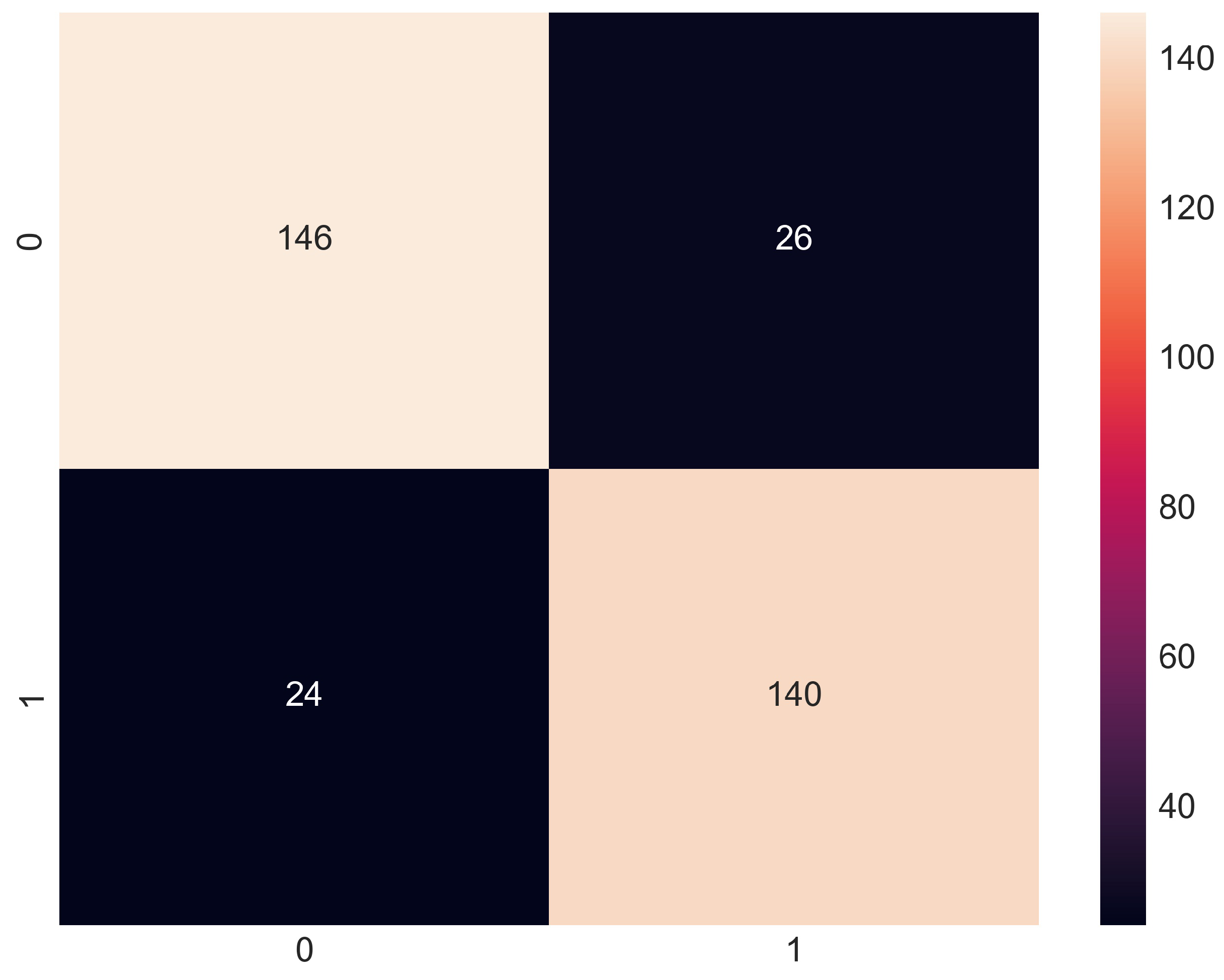
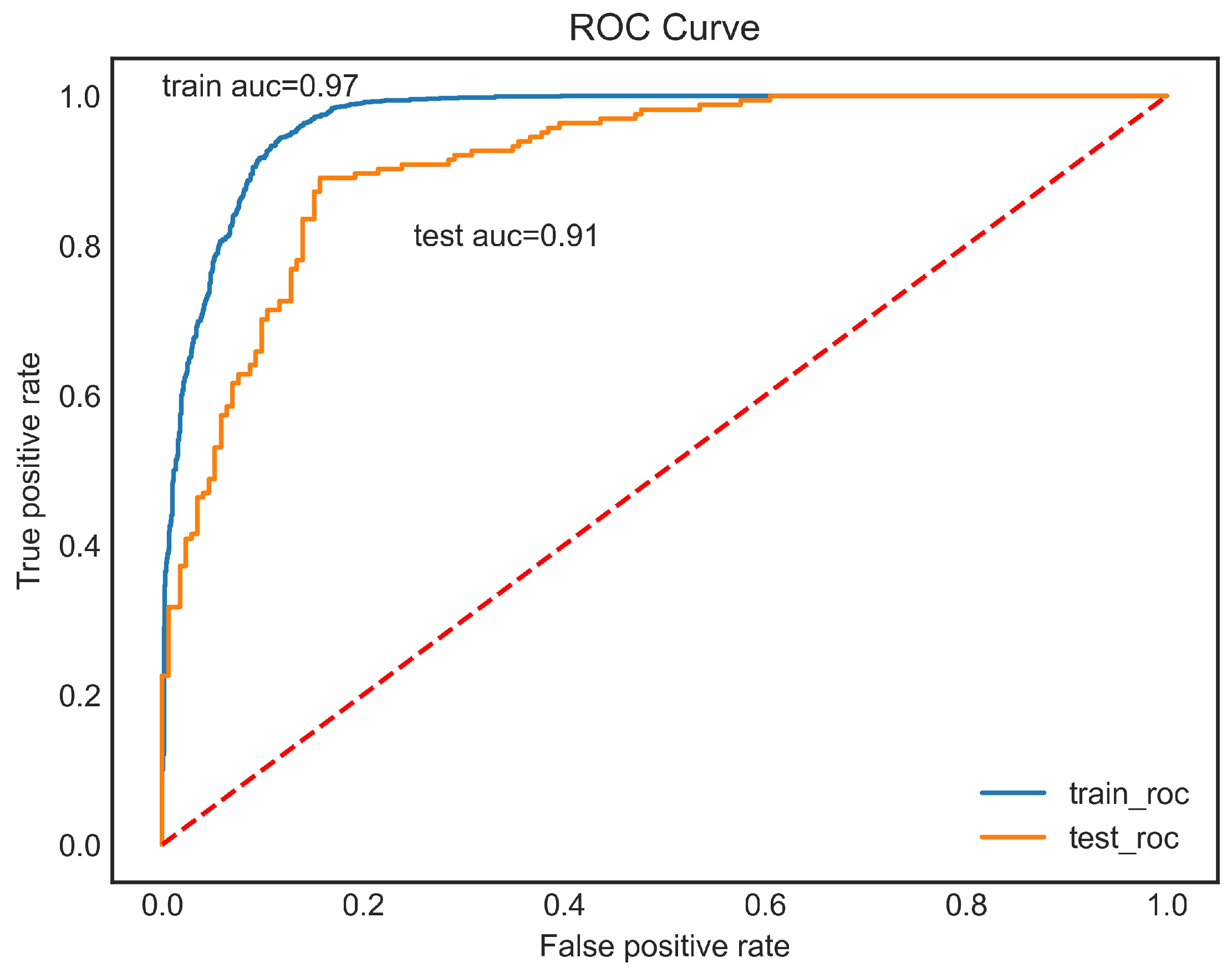
5.2. Evaluation Metrics

To evaluate the model’s effectiveness, we apply five commonly utilized evaluation metrics for classification models: accuracy, precision, recall, F1-score, and AUC (Area Under Curve). First, we construct the binary classification confusion matrix as presented in

Table 2. Confusion matrix for dichotomous model.

	Predicted Value = Negative	Predicted Value = Positive
Actual value = Negative	$TN$	$FP$
Actual value = Positive	$FN$	$TP$

according to the model prediction results.

Then, we calculate the following five metrics. Larger values of these metrics indicate better model performance.

$$Precision=\frac{TP}{TP+FP},Recall=\frac{TP}{TP+FN}$$

(9)

$$Accuracy=\frac{TP+TN}{TP+TN+FP+FN},F1=\frac{2}{\frac{1}{Precision}+\frac{1}{Recall}}$$

(10)

To calculate AUC, we should calculate TRP (True Positive Rate) and FPR (False Positive Rate) first.

$$TPR=Recall=\frac{TP}{TP+FN},FPR=\frac{FP}{FP+TN}$$

(11)

The ROC (Receiver Operating Characteristic) curve is then drawn with FPR as the horizontal axis and TPR as the vertical axis, and AUC is calculated as the area under the ROC curve.

5.3. Model Evaluations

The confusion matrix of LightGBM on the test set is shown in Figure 1. The horizontal axis of Figure 1 represents the predicted value of 0 or 1, the vertical axis represents the actual value of 0 or 1, and the black area represents the number of misclassified instances. The ROC curve is shown in Figure 2, and AUC on the test set can be calculated as 0.91.

In addition, we choose several classic models to compare their performance with LightGBM, including logistic regression (LR), Support Vector Machines (SVM), K-Nearest Neighbors (KNN), Decision Trees (DT), Random Forests (RF), and Deep Neural Networks (DNN). The DNN model is trained by the PyTorch-tabular package [82], and to avoid overfitting, we designed a simple DNN with only two hidden layers containing 64 and 32 neurons, respectively. For the other compared algorithms, we utilize the Scikit-learn package with default parameters. It should be noted that the processing of categorical and numerical features varies when using different models. In particular, when using Decision Trees, Random Forests, and LightGBM models, there is no need to standardize numerical features. However, when using other comparison models, numerical features must be standardized. Additionally, when using LightGBM and DNN models, categorical features only require the label encoder, as the models are capable of processing them on their own. However, for the other comparison models mentioned, categorical features must be converted into dummy variables.

According to the confusion matrix, the average value of accuracy, precision, recall, and F1-score corresponding to all categories on the test set can be calculated, and the results are shown in

Table 3. Evaluation metrics for LightGBM and competitors on the test set.

Model	Accuracy	Precision	Recall	F1
LightGBM	0.85	0.85	0.85	0.85
LR	0.84	0.84	0.84	0.84
SVM	0.84	0.84	0.84	0.84
RF	0.82	0.82	0.81	0.81
DNN	0.80	0.80	0.80	0.80
DT	0.77	0.77	0.77	0.77
KNN	0.74	0.74	0.73	0.73

. The models in Table 3 are ranked based on their performance from best to worst.

Table 3 shows that LightGBM performs the best in terms of accuracy, precision, recall, and F1 score, followed by logistic regression and support vector machines. Although logistic regression is not a black-box model and can directly solve the coefficients of each independent variable, it has a strong assumption (assuming a log-odds relationship between features), and its estimates may still be inaccurate when this assumption is violated. Moreover, logistic regression limits the relationship between features to be monotonic by interpreting the direction and magnitude of the coefficients before the features, whereas the relationship between features is often complex. As we found in the conclusion section of our paper, there is a U-shaped relationship between age and leisure time and an inverted U-shaped relationship between annual household income and leisure time, which logistic regression cannot capture. Furthermore, many statistical theories are based on the assumption that variables are independent of each other, which is difficult to achieve in real-world data. In this regard, tree models may be more suitable than other statistical models. To sum up, the results demonstrate that LightGBM performs well, with favorable scores across multiple metrics, indicating that the selected factors can better explain the changes in residents’ leisure time. Further, SHAP is a better choice to analyze the factors influencing leisure time in Section 6 than some other explanation algorithms such as logistic regression.

6. Analysis of the Changes and Influencing Factors of Leisure Time by Using SHAP

The model built in this paper identifies the relationships between the features very well, which was verified by the excellent results of the evaluation metrics. Therefore, based on the train set, the marginal contributions of each feature for the determination of positive and negative cases are calculated according to the SHAP values of each feature so as to find out how each feature affects the dependent variable.

Beeswarm plots are introduced as a tool to analyze the factors. It should be noted that each point in a beeswarm plot represents a single instance. The different colors signify the various values of the current feature, with blue corresponding to small values and red corresponding to large values. The horizontal axis of the plot indicates SHAP values associated with the features. The magnitude of the SHAP value reflects the feature’s effects on the outcome. A positive SHAP value indicates that the feature leads to a positive impact on the instance’s leisure time, while a negative SHAP value indicates the opposite. Additionally, the higher the SHAP value, the more likely the instance’s leisure time exceeds the median.

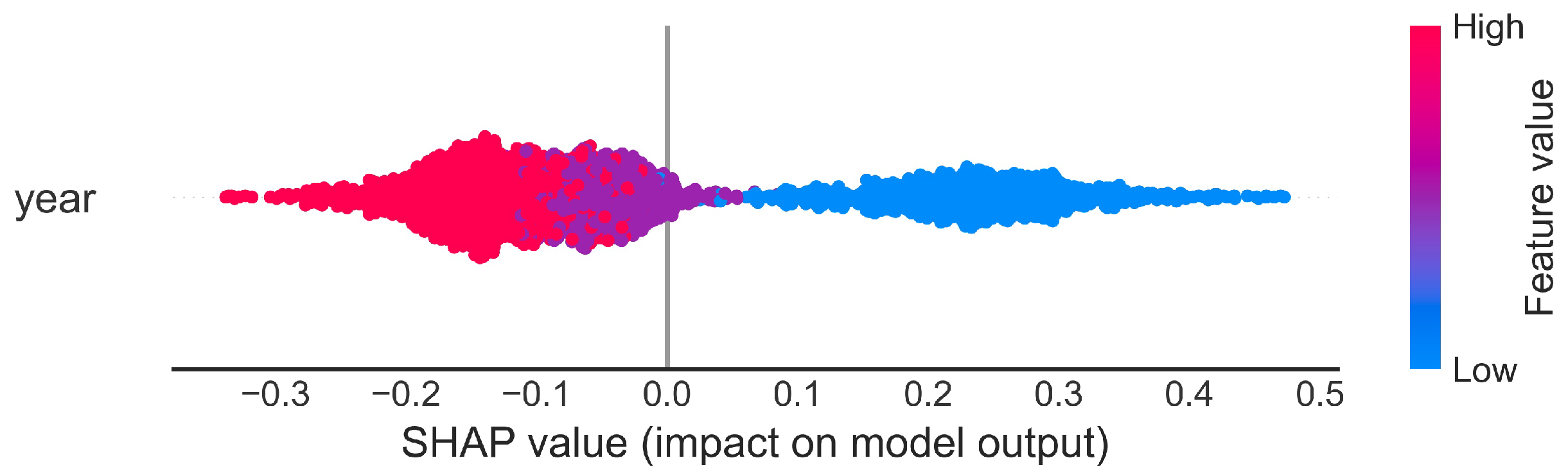
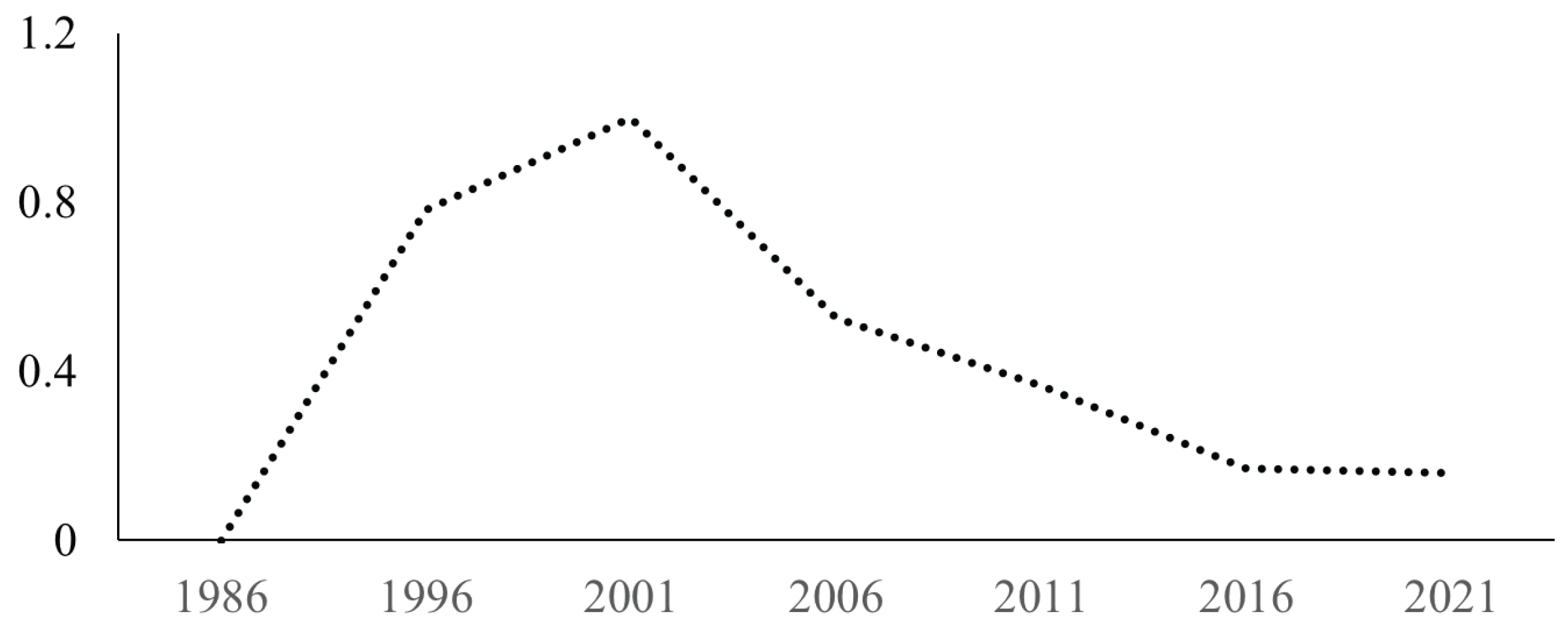
6.1. Changes in Beijing Residents’ Leisure Time over the Last 30 Years

From Figure 3, we find that in the past 10 years from 2011 (blue) to 2021 (red), the SHAP value decreased, indicating that the leisure time of Beijing residents has decreased considerably.

In fact, according to the data from the Beijing Residents’ Time Allocation Survey in 1986, 1996, 2001, 2006, 2011, 2016, and 2021, we can see noticeable changes in leisure time. This demonstrates a trend in which leisure time grew initially and then decreased over the past 30 years in Figure 4. On 1 May 1995, China started implementing the two-day weekend system, and the implementation of the two-day weekend system greatly increased people’s leisure time. Specifically, the average daily leisure time of Beijing residents increased by 1 h and 4 min between 1986 and 1996 thanks to the aforementioned institutional factor. However, under the influence of market factors, the leisure time of residents began to decrease gradually. The average daily leisure time of Beijing residents in 2021 was only 13 min longer than in 1986, while it was 51 min shorter than in 1996.

6.2. Analysis on the Influencing Factors of Beijing Residents’ Leisure Time

6.2.1. Primary Factors Restricting Leisure Time: Work/Study and Housework

The features in Figure 5 are ordered by their significance as calculated by their mean absolute SHAP values. They reflect how the factors influence leisure time in the process of modeling, resulting in the final prediction result.

As shown in Figure 5, all the time allocation characteristics, including work/study time within the system, housework time, essential time for personal life, and commuting time, substantially decrease the amount of leisure time. Work/study time within the system stands out as the most influential factor. It reveals that there are still deficiencies in the current national holiday system and that longer working hours within the system have put a significant strain on leisure time. According to the data from the “China Labor Statistical Yearbook”, the average weekly working hours of Chinese urban employees have been more than 44 h from 2001 to 2020 [83].

Aside from time allocation characteristics, the second most significant influencing factor is age, which is one of the demographic characteristics. Additionally, occupational characteristics play a crucial role in shaping leisure time as well. Despite ranking lower in the order of feature importance, family characteristics do have an effect on leisure time.

Below is a thorough analysis of how demographic, occupational, and family factors influence leisure time.

6.2.2. Age Differences and Gender Inequality in Leisure Time

Age and gender are the most important influencing factors of demographic characteristics, as depicted in Figure 6.

Because the elderly are typically retirees, they tend to have more leisure time. Instances in different gender groups are significantly distributed on both sides of the vertical axis, with males (blue) having more leisure time. It is clear that there is gender inequality in leisure time, which is supported by previous study findings [35]. The SHAP values of years of education primarily range between −0.5 and 0.25, implying that it has an effect on leisure time. As the SHAP values of marital status fluctuate around zero, its effect on leisure time is negligible.

6.2.3. Occupational Heterogeneity in Leisure Time

As illustrated in Figure 7, among occupational characteristics, “enterprise ownership” (i.e., the ownership of the work unit) has the largest impact on leisure time. The color from blue to red denotes “not working, enterprises owned by the whole people, collectively owned enterprises, individual industrial and commercial households, joint ventures, wholly-owned enterprises, joint-stock enterprises and others”. Persons working in enterprises owned by the whole people or in collectively owned enterprises have considerably more leisure time than those in other enterprises, which has been given little emphasis in the previous research. Regarding company size, employees of small companies (blue and purple) have more leisure time than those of large companies (red). From the perspective of occupational category, SHAP values of occupational category vary between −0.6 and 0.6, showing that different occupational categories have varying impacts on leisure time. For instance, management positions and personal occupations (red) are associated with a detrimental effect on leisure time. Additionally, having fewer than two days off per week (also shown in red) significantly reduces leisure time.

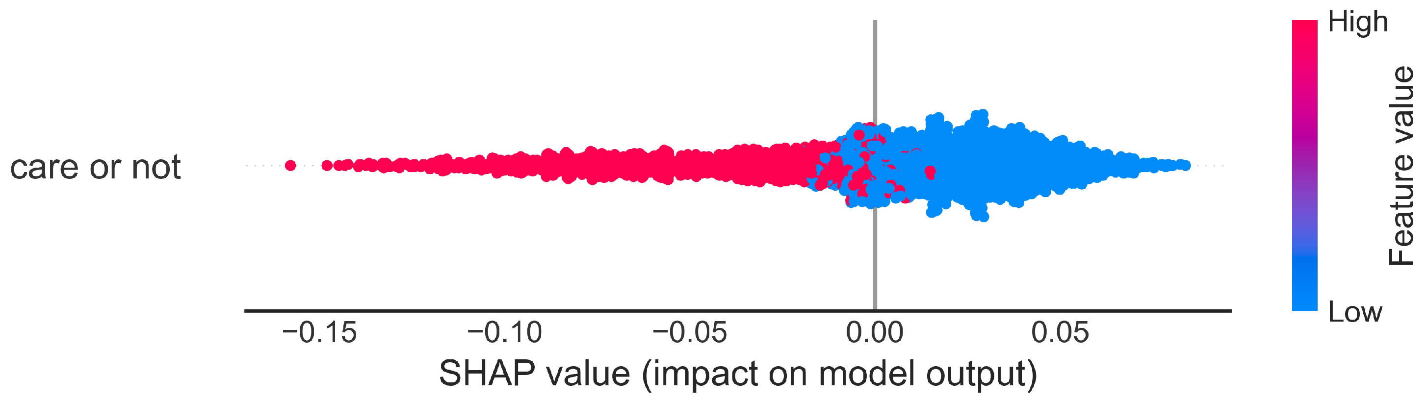
6.2.4. High Income and Caring for Others Squeezing Leisure Time

Annual household income is the most important factor among family characteristics. Figure 8 depicts the major effects of annual household income. The horizontal axis represents the values of the feature, and the left vertical axis represents the SHAP values of the feature, which quantifies the feature’s influence on the LightGBM model’s outcome. The color here has the same meaning as the horizontal axis, namely, corresponding to the feature values.

An upside-down U-shaped curve characterizes the relationship between annual household income and leisure time, as shown in Figure 8. The lowest (blue) and highest income (red) have a significant negative impact on leisure time, presenting a phenomenon of extremely low income and extremely high income accompanied by a lack of leisure time. When the income is less than CNY 30,000, it has a negative impact on leisure time. When the income is between CNY 30,000 and 100,000, it has a positive impact on leisure time, and this positive impact increases with income. However, when the income exceeds CNY 100,000, it begins to have a negative impact on leisure time again, and this influence increases with income.

As for the factor “care or not”, Figure 9 shows that persons without family members to care for (blue) have significantly more leisure time than others. Obviously, when there are people in need of care, it will take up a lot of time. This is consistent with the conclusions of an earlier study that found that when children with chronic diseases need home care, parents’ leisure time is reduced accordingly [55].

6.3. Interaction Effects of the Factors Influencing Beijing Residents’ Leisure Time

To capture the interaction effects between features, we utilize SHAP’s dependency plot for analysis. It can display both the primary and joint impacts of features simultaneously. The interaction effects indicate how two features jointly affect the model’s prediction, and they are displayed through the differing color-coded vertical distribution of SHAP values. The horizontal axis in the dependency plot represents the values of the main feature; the left vertical axis represents the SHAP values of the main feature, which describe the contributions of the main feature to the outcome of LightGBM; the right vertical axis is utilized to describe the interaction effects, illustrating the SHAP values of the interaction feature, and the hue transitions from blue to red as the values of the interaction feature change from small to large.

6.3.1. Gender Inequality Shifts over a Decade

It is evident in Figure 10 that leisure time has decreased over the past ten years from 2011 to 2021. In 2011, women’s SHAP values (red) were lower than men’s (blue), showing that gender inequality was severe with respect to leisure time. In 2016, women’s SHAP values (red) were spread out across the entire vertical axis, indicating that there was no significant difference in leisure time between men and women. In 2021, women’s SHAP values (red) began to be distributed in the upper part of the vertical axis, showing that women’s leisure time had slightly surpassed men’s. The improvement from gender inequality to gender equality has depended on the sustained efforts for gender equality in all fields of society [84].

6.3.2. Gender Inequality Shifts over the Educational Level

It can be seen from Figure 11 that individuals who have graduated but are not currently employed have the most leisure time, while students and current employees have comparatively less leisure time. From the perspective of the fluctuation range of the SHAP values corresponding to the number of years of education, the impact of education level on leisure time shows a decreasing trend with increasing education level, and the direction shows a trend from negative influence to positive influence.

As shown in Figure 11, when the number of years of education is less than nine, women (red) are distributed in the lower half of the vertical axis, indicating that women in this group have less leisure time. When the number of years of education is 9–12, women (red) are uniformly distributed on the vertical axis, showing a tendency toward gender equality. When the number of years of education exceeds 12, most women (red) are distributed in the upper half of the vertical axis, indicating that among highly educated groups, women have more leisure time. This highlights that women have more leisure time as their education level rises. To sum up, education level has a significant moderating effect on gender inequality in leisure time.

6.3.3. Leisure Time Changes for Family Caregivers over a Decade

It can be seen from Figure 12 that in 2011, individuals who needed to care for family members (red) were distributed in the lower half of the vertical axis, implying that they had less leisure time. However, these individuals were distributed in the upper part of the vertical axis in 2016 and 2021, indicating that even with family members in need of care, people have begun to have more leisure time. This improvement may be attributed to economic development, technological progress, and an increase in annual household income, which have provided more advanced methods of assisting people in caring for others, such as hiring professional caregivers [85], utilizing AI intelligent nursing systems [86], etc.

6.3.4. Positive and Negative Effects of Weekly Rest Days

Overall, Figure 13 depicts that the impact of age on leisure time follows a U-shaped pattern. Individuals between the ages of 30 and 40 are in the golden stage of striving for dreams, and they have the least leisure time; as they get older, their leisure time steadily increases.

From the color distribution of the vertical axis in Figure 13, there is a significant interaction effect between age and the weekly rest days. We have a stereotype that fewer vacation days equal less leisure time, and in general, this inference is correct. However, in some cases, fewer vacation days may contribute to a positive change in leisure time. The results in Figure 13 indicate that people between the ages of 20 and 30 who are unable to guarantee two days off weekly (red) are distributed on the upper vertical axis, meaning that they have more leisure time instead. The reason for this phenomenon may be when they must work overtime on weekends, they will look for leisure compensation at other times, such as seeking “retaliatory leisure” by reducing other time, which leads to an increase in leisure time. People aged 30–60 who are unable to take two days off weekly (red) are distributed at the bottom of the vertical axis, suggesting that being unable to take weekend breaks has a major negative impact on leisure time. In general, the failure to implement two days off weekly exerts a marked detrimental impact on leisure time.

7. Conclusions and Discussions

7.1. Main Conclusions

This paper analyzes the changes in residents’ leisure time and the major influencing factors from a machine learning viewpoint in line with the survey data from Beijing residents’ daily time allocation. In general, the time allocation characteristics are the most significant influencing factors. Work time within the system and housework time are the primary drivers of the substantial reduction in leisure time.

In terms of demographic factors, there are age heterogeneity and gender inequalities in leisure time. A U-shaped connection exists between age and leisure time. In the initial stages of life, in order to accumulate capital, individuals sacrificed more and more leisure time as they grew older. As they reach their 40s and beyond, capital accumulation increases, working hours begin to decline after reaching a peak, and leisure activities become more feasible. People’s pursuit of leisure time becomes more urgent as they get older, and as work and life pressures increase, they may consciously increase their leisure time. Gender inequality is evident in leisure time, with men enjoying more leisure time than women. Women may shoulder more housework and caregiving responsibilities, resulting in a continuous erosion of their personal leisure time. Gender inequality has improved considerably over time, and by 2021, there was a trend toward gender equality. Education can reconcile gender inequality, and higher education can serve to promote gender equality.

In terms of occupational factors, they also have a significant influence on leisure time, especially in relation to enterprise ownership. Employees of enterprises owned by the whole people or collectively have more leisure time compared to others. This shows the differences in overtime culture under various enterprise systems, such as the long-standing “996” work system in the Internet industry, in which leisure time is severely constrained by the high-intensity work mode. This is consistent with the conclusion that different occupation categories have different leisure time. The impact of company size is also notable, with large companies exhibiting less leisure time. Interestingly, people aged 20–30 may actively create more leisure time if they have fewer than two days off per week, possibly due to “retaliatory leisure” psychology, which is the active creation of leisure time at the cost of other time. However, in general, taking fewer than two days off per week reduces leisure time.

In terms of family factors, annual household income exhibits an inverted U-shaped relationship with leisure time, whereby individuals with lower incomes (<CNY 30,000) and higher incomes (>CNY 100,000) experience a decrease in leisure time. In contrast, those with annual household incomes between CNY 30,000 and 100,000 experience an increase in leisure time, and this positive impact increases as the income rises. In addition, when there is someone at home who needs to be cared for, the caregiver’s leisure time is consumed. The interaction analysis of joining to “year” shows that with the development of science and technology, the crowding-out effect of taking care of others on leisure time starts to diminish.

7.2. Discussion

Leisure time not only facilitates personal self-development but also stimulates leisure consumption and promotes economic growth. In light of the conclusions of this paper, we put forward the following potential measures to increase personal leisure time.

Reform the current vacation system to ensure the adequate supply of leisure time. The conclusions indicate that leisure time is primarily influenced by working hours. At a national level, the national vacation system determines working hours within the system and serves as the main constraint on the supply of leisure time. The current vacation system can be reformed by the government to increase the overall availability of leisure time. It is important for a country’s vacation system to be in sync with its economic progress; thus, on the basis of certain increase in labor productivity, the length of legal holidays could be appropriately increased. Additionally, to prevent the occurrence of leave-in-lieu and alleviate worker fatigue, one potential solution in developed cities is to implement a four-day-week system, with possible adjustments made based on the actual situation of different enterprises or regions. Furthermore, the results show that having fewer than two days off weekly significantly reduces leisure time, highlighting the challenge of implementing the existing vacation system and ensuring an adequate supply of leisure time. The “996 work system” has even become the standard configuration of Internet companies, and it is difficult to implement both paid leave and two days off per week. To address this problem, relevant reward and punishment policies should be issued to encourage the realization of legal holidays.

Provide personalized leisure products to promote the upgrading of leisure consumption. The results of this paper show that demographic characteristics such as age and gender have a significant impact on leisure time. Accordingly, enterprises can perform user clustering based on the characteristics of various groups and provide personalized leisure products to satisfy different consumer demands. At the market level, material guarantees are necessary to meet people’s leisure consumption needs. For example, the conclusions of this paper demonstrate that women have less leisure time due to increased family obligations. For these groups with special needs, enterprises should create and develop innovative leisure products by leveraging cutting-edge technologies such as 5G and artificial intelligence, which help pave the way for the transformation and enhancement of the leisure industry. This can drive the evolution of the digital economy and travel consumption as well as provide an extensive variety of online services. The supply of online products such as “cloud music” and “cloud exhibition” can also be increased, enabling people to conveniently engage in leisure activities at any time and from any location. In particular, for elderly adults, community-based programs that provide leisure activities at home can create a fulfilling and enjoyable lifestyle for them in their twilight years.

Advocate a proper perception of leisure and stimulate potential leisure needs. The findings suggest notable dissimilarities in leisure time among people with different occupational characteristics. To alter this professional imbalance in leisure time, the government should first take the lead in enforcing and penalizing practices, providing channels for employees to report violations, and safeguarding employees’ rights and interests. Second, we must promote the perception of leisure across society to encourage employees to pursue reasonable leisure time actively. From a demand standpoint, it is essential to provide a basic guarantee to strengthen people’s leisure needs. Highlight the fact that leisure time is the guarantee for people to live a happy life and do not put “leisure” and “labor” in opposition. The purpose of “labor” is to free up more time and money for leisure activities, which not only relax the body and mind but also help people achieve self-reflection and self-improvement, allowing them to dedicate themselves to “labor” more effectively. We should enhance public awareness; promote diverse and healthy leisure options; create a favorable environment for high-end leisure, cultural, and tourism activities; and raise awareness of the importance of leisure by organizing leisure conferences and publishing relevant leisure tourism manuals.

Despite conducting a comprehensive analysis of the effects of time allocation factors, demographic factors, occupational factors, and family factors on leisure time from a micro perspective, this paper has several research limitations. Firstly, due to technical constraints, the SHAP approach utilized in this paper provides insight into how features affect LightGBM model predictions, but it may not reveal the true causal relationships between features and outcomes in the real world. Although this does not undermine the conclusions drawn in this paper, we intend to utilize other causal inference methods such as Double Machine Learning to quantify the causal effects and evaluate the intervention effects by making counterfactual predictions in future studies. Secondly, owing to data unavailability, this paper only considers Beijing as a case study, yet leisure time varies across regions. Thereby, in the future, we aim to incorporate more regions for comparative analysis.

References

1. Bouwer, J.; Van Leeuwen, M. Philosophy of Leisure: Foundations of the Good Life; Routledge: New York, NY, USA, 2017. [Google Scholar]
2. Opić, S.; Đuranović, M. Leisure time of young due to some socio-demographic characteristics. Procedia-Soc. Behav. Sci. 2014, 159, 546–551. [Google Scholar] [CrossRef]
3. Cui, D.; Wei, X.; Wu, D.; Cui, N.; Nijkamp, P. Leisure time and labor productivity: A new economic view rooted from sociological perspective. Economics 2019, 13, 1–24. [Google Scholar] [CrossRef]
4. Dimitrova, R. Trends Analysis to Use Leisure Time. Econ. Financ. 2019, 6, 28–38. [Google Scholar]
5. Anderson, L.S.; Heyne, L.A. Flourishing through leisure: An ecological extension of the leisure and well-being model in therapeutic recreation strengths-based practice. Ther. Recreat. J. 2012, 46, 129. [Google Scholar]
6. Bittman, M. Social participation and family welfare: The money and time costs of leisure in Australia. Soc. Policy Adm. 2002, 36, 408–425. [Google Scholar] [CrossRef]
7. Cook, D.T. Leisure and consumption. In A Handbook of Leisure Studies; Rojek, C., Shaw, S., Veal, A., Eds.; Palgrave Macmillan: London, UK, 2006; pp. 304–316. [Google Scholar]
8. Stebbins, R. Leisure and Consumption: Common Ground/Separate Worlds; Palgrave Macmillan: New York, NY, USA, 2009. [Google Scholar]
9. Sullivan, O.; Gershuny, J. Inconspicuous consumption: Work-rich, time-poor in the liberal market economy. J. Consum. Cult. 2004, 4, 79–100. [Google Scholar] [CrossRef]
10. Vickery, C. The time-poor: A new look at poverty. J. Hum. Resour. 1977, 12, 27–48. [Google Scholar] [CrossRef]
11. Lin, K. Tech worker organizing in China: A new model for workers battling a repressive state. In New Labor Forum; SAGE Publications Sage CA: Los Angeles, CA, USA, 2020; Volume 29, pp. 52–59. [Google Scholar]
12. Mapped: Which Countries Get the Most Paid Vacation Days? Available online: https://www.visualcapitalist.com/cp/mapped-which-countries-get-the-most-paid-vacation-days/ (accessed on 28 April 2023).
13. Kuykendall, L.; Boemerman, L.; Zhu, Z. The importance of leisure for subjective well-being. In Handbook of Well-Being; DEF Publishers: Salt Lake City, UT, USA, 2018. [Google Scholar]
14. Yasarturk, F.; Akyüz, H.; Karatas, I.; Turkmen, M. The relationship between free time satisfaction and stress levels of elite-level student-wrestlers. Educ. Sci. 2018, 8, 133. [Google Scholar] [CrossRef]
15. Liu, H.; Da, S. The relationships between leisure and happiness-A graphic elicitation method. Leis. Stud. 2020, 39, 111–130. [Google Scholar] [CrossRef]
16. Greaney, V.; Hegarty, M. Correlates of leisure-time reading. J. Res. Read. 1987, 10, 3–20. [Google Scholar] [CrossRef]
17. Roberts, K. Leisure in Contemporary Society; Cabi: Wallingford, UK, 2006. [Google Scholar]
18. Voorpostel, M.; Van Der Lippe, T.; Gershuny, J. Spending time together—Changes over four decades in leisure time spent with a spouse. J. Leis. Res. 2010, 42, 243–265. [Google Scholar] [CrossRef]
19. Shaw, S.M.; Dawson, D. Purposive leisure: Examining parental discourses on family activities. Leis. Sci. 2001, 23, 217–231. [Google Scholar] [CrossRef]
20. Leitner, M.J.; Leitner, S.F. Leisure Enhancement; Haworth Press: Binghamton, NY, USA, 2004. [Google Scholar]
21. Žumárová, M. Computers and children’s leisure time. Procedia-Soc. Behav. Sci. 2015, 176, 779–786. [Google Scholar] [CrossRef]
22. Schulz, J.; Watkins, M. The development of the leisure meanings inventory. J. Leis. Res. 2007, 39, 477–497. [Google Scholar] [CrossRef]
23. Iwasaki, Y. Pathways to meaning-making through leisure-like pursuits in global contexts. J. Leis. Res. 2008, 40, 231–249. [Google Scholar] [CrossRef]
24. Soyer, F.; Demirel, M.; Kacay, Z.; Ayhan, C.; Demirel, D.H. Examination of the Opinions of University Students on the Meaning of Leisure Time and the Lesson Study Approaches. Khazar J. Humanit. Soc. Sci. 2017, 18–31. [Google Scholar]
25. Auger, D. The diverse meanings of leisure/Les diverses significations du loisir. Soc. Leis. 2016, 39, 173–176. [Google Scholar] [CrossRef]
26. Seibel, S.; Volmer, J.; Syrek, C.J. Get a taste of your leisure time: The relationship between leisure thoughts, pleasant anticipation, and work engagement. Eur. J. Work Organ. Psychol. 2020, 29, 889–906. [Google Scholar] [CrossRef]
27. Burda, M.C.; Hamermesh, D.S.; Weil, P. Total Work, Gender and Social Norms; NBER Working Papers No. 13000; National Bureau of Economic Research: Cambridge, MA, USA, 2007. [Google Scholar]
28. Andronis, L.; Maredza, M.; Petrou, S. Measuring, valuing and including forgone childhood education and leisure time costs in economic evaluation: Methods, challenges and the way forward. Soc. Sci. Med. 2019, 237, 112475. [Google Scholar] [CrossRef]
29. Clark, B.; Chatterjee, K.; Martin, A.; Davis, A. How commuting affects subjective wellbeing. Transportation 2020, 47, 2777–2805. [Google Scholar] [CrossRef]
30. Pepin, J.R.; Sayer, L.C.; Casper, L.M. Marital status and mothers’ time use: Childcare, housework, leisure, and sleep. Demography 2018, 55, 107–133. [Google Scholar] [CrossRef] [PubMed]
31. Wales, T.J.; Woodland, A.D. Estimation of the allocation of time for work, leisure, and housework. Econom. J. Econom. Soc. 1977, 115–132. [Google Scholar] [CrossRef]
32. Zuzanek, J. Work, leisure, time-pressure and stress. In Work and Leisure; Haworth, J.T., Veal, A.J., Eds.; Routledge: London, UK, 2004; pp. 123–144. [Google Scholar]
33. Thrane, C. Men, women, and leisure time: Scandinavian evidence of gender inequality. Leis. Sci. 2000, 22, 109–122. [Google Scholar] [CrossRef]
34. Becker, G.S. Human capital, effort, and the sexual division of labor. J. Labor Econ. 1985, 3, S33–S58. [Google Scholar] [CrossRef]
35. Bittman, M.; Wajcman, J. The rush hour: The character of leisure time and gender equity. Soc. Forces 2000, 79, 165–189. [Google Scholar] [CrossRef]
36. Lydeka, Z.; Tauraitė, V. Evaluation of the time allocation for work and personal life among employed population in Lithuania from gender perspective. Eng. Econ. 2020, 31, 104–113. [Google Scholar] [CrossRef]
37. Haller, M.; Hadler, M.; Kaup, G. Leisure time in modern societies: A new source of boredom and stress? Soc. Indic. Res. 2013, 111, 403–434. [Google Scholar] [CrossRef]
38. Miller, Y.D.; Brown, W.J. Determinants of active leisure for women with young children—An “ethic of care” prevails. Leis. Sci. 2005, 27, 405–420. [Google Scholar] [CrossRef]
39. Bauer, F.; Groß, H.; Oliver, G.; Sieglen, G.; Smith, M. Time Use and Work–Life Balance in Germany and the UK; Anglo-German Foundation for the Study of Industrial Society: London, UK, 2007. [Google Scholar]
40. Lee, Y.G.; Bhargava, V. Leisure time: Do married and single individuals spend it differently? Fam. Consum. Sci. Res. J. 2004, 32, 254–274. [Google Scholar] [CrossRef]
41. Zuzanek, J. Social differences in leisure behavior: Measurement and interpretation. Leis. Sci. 1978, 1, 271–293. [Google Scholar] [CrossRef]
42. Dyble, M.; Thorley, J.; Page, A.E.; Smith, D.; Migliano, A.B. Engagement in agricultural work is associated with reduced leisure time among Agta hunter-gatherers. Nat. Hum. Behav. 2019, 3, 792–796. [Google Scholar] [CrossRef]
43. Shaw, B.A.; Liang, J.; Krause, N.; Gallant, M.; McGeever, K. Age differences and social stratification in the long-term trajectories of leisure-time physical activity. J. Gerontol. Ser. Psychol. Sci. Soc. Sci. 2010, 65, 756–766. [Google Scholar] [CrossRef]
44. Agahi, N.; Ahacic, K.; Parker, M.G. Continuity of leisure participation from middle age to old age. J. Gerontol. Ser. B: Psychol. Sci. Soc. Sci. 2006, 61, S340–S346. [Google Scholar] [CrossRef]
45. Andersen, L.B.; Schnohr, P.; Schroll, M.; Hein, H.O. All-cause mortality associated with physical activity during leisure time, work, sports, and cycling to work. Arch. Intern. Med. 2000, 160, 1621–1628. [Google Scholar] [CrossRef]
46. Werneck, A.O.; Oyeyemi, A.L.; Araújo, R.H.; Barboza, L.L.; Szwarcwald, C.L.; Silva, D.R. Association of public physical activity facilities and participation in community programs with leisure-time physical activity: Does the association differ according to educational level and income? BMC Public Health 2022, 22, 279. [Google Scholar] [CrossRef]
47. Kirk, M.A.; Rhodes, R.E. Occupation correlates of adults’ participation in leisure-time physical activity: A systematic review. Am. J. Prev. Med. 2011, 40, 476–485. [Google Scholar] [CrossRef]
48. Ganzeboom, H.B.; Treiman, D.J. Internationally comparable measures of occupational status for the 1988 International Standard Classification of Occupations. Soc. Sci. Res. 1996, 25, 201–239. [Google Scholar] [CrossRef]
49. Wei, J.; Li, Y.; Liu, X.; Du, Y. Enterprise characteristics and external influencing factors of sustainable innovation: Based on China’s innovation survey. J. Clean. Prod. 2022, 372, 133461. [Google Scholar] [CrossRef]
50. Aleksynska, M.; Berg, J.; Foden, D.; Johnston, H.; Parent-Thirion, A.; Vanderleyden, J.; Vermeylen, G. Working Conditions in a Global Perspective; Research report/Eurofound; Publications Office of the European Union: Luxembourg, 2019. [Google Scholar]
51. Vandelanotte, C.; Short, C.; Rockloff, M.; Di Millia, L.; Ronan, K.; Happell, B.; Duncan, M.J. How do different occupational factors influence total, occupational, and leisure-time physical activity? J. Phys. Act. Health 2015, 12, 200–207. [Google Scholar] [CrossRef]
52. Gu, J.K.; Charles, L.E.; Ma, C.C.; Andrew, M.E.; Fekedulegn, D.; Hartley, T.A.; Violanti, J.M.; Burchfiel, C.M. Prevalence and trends of leisure-time physical activity by occupation and industry in US workers: The National Health Interview Survey 2004–2014. Ann. Epidemiol. 2016, 26, 685–692. [Google Scholar] [CrossRef]
53. Firestone, J.; Shelton, B.A. A comparison of women’s and men’s leisure time: Subtle effects of the double day. Leis. Sci. 1994, 16, 45–60. [Google Scholar] [CrossRef]
54. Yasartürk, F.; Akyüz, H.; Gönülates, S. The Investigation of the Relationship between University Students’ Levels of Life Quality and Leisure Satisfaction. Univers. J. Educ. Res. 2019, 7, 739–745. [Google Scholar] [CrossRef]
55. Hatzmann, J.; Peek, N.; Heymans, H.; Maurice-Stam, H.; Grootenhuis, M. Consequences of caring for a child with a chronic disease: Employment and leisure time of parents. J. Child Health Care 2014, 18, 346–357. [Google Scholar] [CrossRef] [PubMed]
56. Fernandez-Crehuet, J.M.; Gimenez-Nadal, J.I.; Reyes Recio, L.E. The national work–life balance index©: The European case. Soc. Indic. Res. 2016, 128, 341–359. [Google Scholar] [CrossRef]
57. Shen, H.; Wang, Q.; Ye, C.; Liu, J.S. The evolution of holiday system in China and its influence on domestic tourism demand. J. Tour. Futur. 2018, 4, 139–151. [Google Scholar] [CrossRef]
58. York, Q.Y.; Ye, B.H. Research note: Why gold is so stronghold, revealing the mechanism of China’s golden week holiday system. Leis. Stud. 2018, 37, 352–358. [Google Scholar] [CrossRef]
59. Wang, P.; Wei, X.; Yingwei, X.; Xiaodan, C. The impact of residents’ leisure time allocation mode on individual subjective well-being: The case of China. Appl. Res. Qual. Life 2022, 17, 1831–1866. [Google Scholar] [CrossRef]
60. Gali, J. Technology, employment, and the business cycle: Do technology shocks explain aggregate fluctuations? Am. Econ. Rev. 1999, 89, 249–271. [Google Scholar] [CrossRef]
61. Dridea, C.; Sztruten, G. Free time-the major factor of influence for leisure. Rom. Econ. Bus. Rev. 2010, 5, 208. [Google Scholar]
62. Min, J.; Jin, H. Analysis on Essence, Types and Characteristics of Leisure Sports. Mod. Appl. Sci. 2010, 4, 99. [Google Scholar] [CrossRef]
63. Rätsel, S. Revisiting the neoclassical theory of labour supply: Disutility of labour, working hours, and happiness. Work. Pap. Ser. 2009. [Google Scholar]
64. Yaniv, G. Workaholism and marital estrangement: A rational-choice perspective. Math. Soc. Sci. 2011, 61, 104–108. [Google Scholar] [CrossRef]
65. Al Daoud, E. Comparison between XGBoost, LightGBM and CatBoost using a home credit dataset. Int. J. Comput. Inf. Eng. 2019, 13, 6–10. [Google Scholar]
66. Zhang, L.; Liu, M.; Qin, X.; Liu, G. Succinylation site prediction based on protein sequences using the IFS-LightGBM (BO) model. Comput. Math. Methods Med. 2020, 2020, 8858489. [Google Scholar] [CrossRef]
67. Sun, X.; Liu, M.; Sima, Z. A novel cryptocurrency price trend forecasting model based on LightGBM. Financ. Res. Lett. 2020, 32, 101084. [Google Scholar] [CrossRef]
68. Molnar, C. Interpretable Machine Learning. Available online: https://originalstatic.aminer.cn/misc/pdf/Molnar-interpretable-machine-learning_compressed.pdf (accessed on 28 April 2023).
69. Lundberg, S.M.; Lee, S.I. A unified approach to interpreting model predictions. In Proceedings of the 31st Conference on Neural Information Processing Systems (NIPS 2017), Long Beach, CA, USA, 4–9 December 2017; pp. 4765–4774. [Google Scholar]
70. Zhang, J.; Ma, X.; Zhang, J.; Sun, D.; Zhou, X.; Mi, C.; Wen, H. Insights into geospatial heterogeneity of landslide susceptibility based on the SHAP-XGBoost model. J. Environ. Manag. 2023, 332, 117357. [Google Scholar] [CrossRef]
71. Wen, X.; Xie, Y.; Wu, L.; Jiang, L. Quantifying and comparing the effects of key risk factors on various types of roadway segment crashes with LightGBM and SHAP. Accid. Anal. Prev. 2021, 159, 106261. [Google Scholar] [CrossRef]
72. Friedman, J.H. Greedy function approximation: A gradient boosting machine. Ann. Stat. 2001, 29, 1189–1232. [Google Scholar] [CrossRef]
73. Ke, G.; Meng, Q.; Finley, T.; Wang, T.; Chen, W.; Ma, W.; Ye, Q.; Liu, T.Y. Lightgbm: A highly efficient gradient boosting decision tree. In Proceedings of the 31st Conference on Neural Information Processing Systems (NIPS 2017), Long Beach, CA, USA, 4–9 December 2017; pp. 3147–3155. [Google Scholar]
74. Chen, T.; Guestrin, C. Xgboost: A scalable tree boosting system. In Proceedings of the 22nd ACM Sigkdd International Conference on Knowledge Discovery and Data Mining, San Francisco, CA, USA, 13–17 August 2016; pp. 785–794. [Google Scholar]
75. Alabdullah, A.A.; Iqbal, M.; Zahid, M.; Khan, K.; Amin, M.N.; Jalal, F.E. Prediction of rapid chloride penetration resistance of metakaolin based high strength concrete using lightGBM and XGBoost models by incorporating SHAP analysis. Constr. Build. Mater. 2022, 345, 128296. [Google Scholar] [CrossRef]
76. Shapley, L.S. 17. A Value for n-Person Games. In Contributions to the Theory of Games (AM-28), Volume II; Kuhn, H.W., Tucker, A.W., Eds.; Princeton University Press: Princeton, NJ, USA, 1953; pp. 307–318. [Google Scholar]
77. Lundberg, S.M.; Erion, G.G.; Lee, S.I. Consistent individualized feature attribution for tree ensembles. arXiv 2018, arXiv:1802.03888. [Google Scholar]
78. Lundberg, S.M.; Nair, B.; Vavilala, M.S.; Horibe, M.; Eisses, M.J.; Adams, T.; Liston, D.E.; Low, D.K.W.; Newman, S.F.; Kim, J.; et al. Explainable machine-learning predictions for the prevention of hypoxaemia during surgery. Nat. Biomed. Eng. 2018, 2, 749–760. [Google Scholar] [CrossRef] [PubMed]
79. Lundberg, S.M.; Erion, G.; Chen, H.; DeGrave, A.; Prutkin, J.M.; Nair, B.; Katz, R.; Himmelfarb, J.; Bansal, N.; Lee, S.I. From local explanations to global understanding with explainable AI for trees. Nat. Mach. Intell. 2020, 2, 56–67. [Google Scholar] [CrossRef] [PubMed]
80. Lee, S.; McCann, D.; Messenger, J.C. Working Time around the World: Trends in Working Hours, Laws, and Policies in a Global Comparative Perspective; International Labour Office: Geneva, Switzerland, 2007. [Google Scholar]
81. Pedregosa, F.; Varoquaux, G.; Gramfort, A.; Michel, V.; Thirion, B.; Grisel, O.; Blondel, M.; Prettenhofer, P.; Weiss, R.; Dubourg, V.; et al. Scikit-learn: Machine learning in Python. J. Mach. Learn. Res. 2011, 12, 2825–2830. [Google Scholar]
82. Joseph, M. Pytorch tabular: A framework for deep learning with tabular data. arXiv 2021, arXiv:2104.13638. [Google Scholar]
83. Department of Population and Employment Statistic National Bureau of Statistics; Department of Planning and Finance, Ministry of Human Resources and Social Security. China Labor Statistical Yearbook; China Statistics Press: Beijing, China, 2021.
84. Alarcón, D.M.; Cole, S. No sustainability for tourism without gender equality. J. Sustain. Tour. 2019, 27, 903–919. [Google Scholar] [CrossRef]
85. Seidel, D.; Thyrian, J.R. Burden of caring for people with dementia—Comparing family caregivers and professional caregivers. A descriptive study. J. Multidiscip. Healthc. 2019, 12, 655–663. [Google Scholar] [CrossRef]
86. Higgins, O.; Short, B.L.; Chalup, S.K.; Wilson, R.L. Artificial intelligence (AI) and machine learning (ML) based decision support systems in mental health: An integrative review. Int. J. Ment. Health Nurs. 2023. [Google Scholar] [CrossRef]
Figure 1. Confusion matrix for LightGBM on the test set.
Mathematics 11 02371 g001
Figure 2. ROC curve for LightGBM on the train set and test set.
Mathematics 11 02371 g002
Figure 3. Beeswarm plot of the effects of “year”.
Mathematics 11 02371 g003
Figure 4. Changes in leisure time over the past 30 years (leisure time has been normalized by Min–Max).
Mathematics 11 02371 g004
Figure 5. Beeswarm plot of feature importance ranking.
Mathematics 11 02371 g005
Figure 6. Beeswarm plot of the effects of demographic factors.
Mathematics 11 02371 g006
Figure 7. Beeswarm plot of the effects of occupational factors.
Mathematics 11 02371 g007
Figure 8. Scatter plot of the effects of annual household income.
Mathematics 11 02371 g008
Figure 9. Beeswarm plot of the effects of “care or not”.
Mathematics 11 02371 g009
Figure 10. Interaction effects of “year” and “gender”.
Mathematics 11 02371 g010
Figure 11. Interaction effects of “education” and “gender”.
Mathematics 11 02371 g011
Figure 12. Interaction effects of “year” and “care or not”.
Mathematics 11 02371 g012
Figure 13. Interaction effects of “age” and “weekly rest days”.
Mathematics 11 02371 g013