1. Introduction
The increase in the number of motor vehicles is an important manifestation of social and economic development and improvement in people’s living standards; however, the continuous increase in the number of motor vehicles has entailed pollution problems. The use maintenance and scrapping of motor vehicles entail environmental problems [
1]. For example, exhaust gas problems caused by the use of motor vehicles (fuel vehicles) have increased demand for charging, leading to increased load on the power grid, and to pollution problems caused by increased demand for power generation at the source level (new energy vehicles or electric cars), tire wear particles (TWP) problems caused by low-tech tires, increased unit energy consumption and increased accident rates, due to tire wear air pollution, soil pollution and water pollution caused by dismantling, recycling and landfilling of scrapped cars, due to age or other reasons [
2].
The harm caused by greenhouse gases is well-known, and the problem of exhaust emissions caused by the operation of internal combustion engines has become the focus of policy formulation by governments around the world. A series of policies have been successfully implemented, to reduce this aspect of traffic-related exhaust emissions. With the further promotion and use of new energy vehicles, PM (particulate matter) exhaust emissions will be further alleviated. However, the attention being paid to pollution caused by waste generated by friction between tires and the ground is still insufficient. For a long time, research on microplastics has focused only on thermoplastic materials such as polyethylene or polystyrene, without considering elastomeric materials, such as rubber. According to ISO’s definition, rubber is not included in the definition of plastic. By contrast, some academics have suggested a broader and more commonsense definition of microplastics that includes common macromolecular materials: hence, the inclusion of rubber [
3].
The technical content of tires should receive attention, for its impact on the environment and driving safety. A tire is a round, black object that seems to have little technical content, but is not cheap. Consumers usually make tire purchase decisions based on price. In fact, in a typical radial passenger car tire, there are 20 or more components, and 15 or more rubber compounds. Tires are highly engineered structural composites, the performance design of which must meet the smoothness handling and traction standards of automobile manufacturers, as well as customer expectations of quality and performance. A medium-sized car’s tires rotate more than 1200 times per kilometer, and within 50,000 km each tire component undergoes more than 24 million loading and unloading cycles, requiring extremely high endurance [
4]. The waste generated by the friction between a single tire and the ground seems insignificant, but on a global scale it is considerable, and it is predicted that, in the near future, pollution caused by this type of frictional wear will not decrease [
2,
5].
Microplastics are considered a global threat by many studies, due to their widespread presence in all regions inhabited by humans, as a result of the extensive use of automobiles. Microplastics permeate all ecosystems, and have the potential to impact the health of aquatic and terrestrial organisms, including humans, through various exposure pathways, such as food chains, drinking water and air [
6,
7,
8,
9]. According to academic and industry definitions, microplastics are polymer materials with a maximum diameter of no more than 5 mm, which are insoluble in water, and have an extremely low degradation rate [
10]. Particles released from tire wear fit this description, and were recognized as a new type of potential pollutant by industry scholars as early as the 1970s [
11]. Because of their insoluble and non-degradable nature, the distribution and residues of microplastics remain highly uncertain after decades of self-processing in nature [
12]. The composition of tire wear varies, depending on the brand and intended use of the original tire. A typical passenger tire may contain 30 types of styrene–butadiene rubber, 8 types of natural rubber, 8 types of carbon black and over 40 different chemicals, as well as polyester and nylon fibers [
13,
14]. Different ingredient ratios result in a large number of tire formulations. The main components include 40–60% rubber content (including synthetic and natural rubber), 20–35% fillers (carbon black and silica) and 12–15% various oils [
15]. The physical and chemical properties of tire wear particles (TWP) have not been sufficiently studied, as they can also absorb materials from the road and the surrounding environment [
13]. The rate of tire wear particle (TWP) production due to road wear has been reported to vary between 10% to 50%, which may be related to road surface materials, including asphalt, road dust, gravel, oil, and plasticizers, all of which have an impact on the production of TWPs [
9]. The amount and rate of tire wear particle production varies according to a number of factors, and, according to studies, increases due to vehicle loads, under- or over-inflation of tires, wheel alignment deviations, wheel position (front wheels wear first), transitional exposure to the elements, sudden braking, acceleration or sustained high speeds [
10,
16]. Kole et al. estimated data on TWPs from tire wear: based on the global population and the number of motor vehicles of all types, they estimated that emissions have reached nearly 6 million tons per year [
16], equivalent to about 0.81 kg per capita per year. Some components of tires have been proven to be toxic; therefore, it is necessary to reduce the amount of these harmful substances released into the external environment [
17,
18,
19].
As cars travel, the continuous wear of tires releases microplastic particles into the environment. Excessive tire wear can also affect driving safety. According to statistics from the World Health Organization, more than 1.3 million people die each year from road traffic accidents. Road traffic accident is one of the top ten causes of death for all age groups, and this trend is on the rise, especially for young people [
20]. The health of a moving vehicle’s tires is only one of the causes of road traffic accidents, but road traffic accidents related to tire health problems can lead to more grievous injury to life and damage to property [
21]. A study using seven years of Louisiana crash data showed that sudden tire failure and excessive tire wear significantly affect the severity of road crashes [
22]. A substantial proportion of traffic accidents are caused by lack of vehicle maintenance, and by tire defects. For example, data from the United States show that in the National Motor Vehicle Crash Causation Survey (NMVCCS), conducted from 2005 to 2007, out of approximately 44,000 traffic accidents related to vehicle defects, more than 15,000 were related to tire defects, accounting for over 35%. According to a report from the National Highway Traffic Safety Administration (NHTSA), an average of nearly 11,000 tire-related motor vehicle accidents occur annually in the United States, resulting in approximately 200 fatalities. In 2017, a total of 738 people died in tire-related traffic accidents on American roads. These fatalities have drawn attention to the study of factors that cause tire failure, and to the analysis of the severity of injuries in tire-related accidents.
Therefore, it is necessary to develop green tires with better environmental performance (e.g., more wear-resistant, better air-tightness and better anti-burst performance), both for environmental protection and for the safety of people and property. Because of the increasingly serious environmental problems and the systematic promotion of the concept of green development, the cultivation of a green supply chain operation model is also gaining more and more attention from government, and from upstream and downstream enterprises in the supply chain.
The development and production of green tires can be traced back to 1992, when Michelin produced the first recognized green tire. This product strategy, which focuses on environmental protection, has brought Michelin both economic and social benefits [
23]. In 2012, the European Union officially implemented a European tire labeling Regulation. This Regulation requires that car tires, light truck tires, truck tires and bus tires sold in the EU must have a label indicating the tire’s rolling resistance (fuel efficiency), rolling noise and wet grip performance levels. The introduction of this regulation is seen as a sign of the official promotion of high-quality green tires [
24]. Subsequently, various countries have introduced labeling regulations related to tire rolling resistance. In 2016, China also issued a tire labelling law requiring that energy consumption, wet grip and noise be indicated on tires. Although green tires are relatively more expensive than ordinary tires, their superior performance, more user-friendly experience, lower fuel consumption and more environmentally friendly energy-saving features have made them increasingly popular among consumers.
Generally speaking, the development of green products requires relatively high research and development costs, and their selling prices are also higher. As China’s economy has entered a new stage in recent years, and its society has increasingly valued green environmental protection, consumers have also paid more attention to the low-carbon economy. Improving the greenness of products is one of the important ways to achieve this. Many studies have pointed out that today’s consumer concept makes buyers willing to choose products with carbon emission labels. Market demand changes with consumer willingness, prompting product manufacturers to innovate technology to produce low-carbon and environmentally friendly green products, to enhance their competitiveness in the market [
25].
The green product market is still in its infancy. In order to further expand the market, and to gain a competitive advantage while also making long-term plans, it is necessary for companies to actively invest in the research and development of green products, and to produce green environmental protection products that meet government policy guidance, social development and consumer preferences. This article proposes that when green product manufacturers increase investment in research and development, and reduce carbon emissions, retailers can also effectively participate, which is conducive to promoting benign cooperation between manufacturers and retailers, increasing economic income and further enhancing the core competitiveness of enterprises. We conducted research on the current situation of green economy and carbon emissions development, and, based on systematic observations of green supply chain repurchase contracts, combined with supply chain theory, we conducted in-depth research on supply chain repurchase coordination and cost-sharing. We have striven to propose suggestions for effectively ensuring the coordination of the green supply chain system, and to provide research support for further enhancing the competitive advantage of the green supply chain in the rapid development process of the current market economy.
Based on the analysis above, there are three important questions: (1) When the random demand is related to the product green level, and considering carbon emissions trading, how to coordinate the green supply chain? (2) How does carbon emissions trading affect supply chain profit and coordination? (3) How to share the cost between the parties in the green supply chain? The main purpose and significance of this study was to investigate these questions. The main contribution and results of this work are as follows:
Unlike the findings of the classic literature, random demand is related to the product green level. In addition, the cost is shared between the manufacturer and the retailer. Under the green supply chain buyback contract, both the product green level and order quantity need to be decided. In order to coordinate the green supply chain, the manufacturer needs to share both the goods salvage risk and the cost;
Under the green supply chain buyback contract, we found that both the wholesale price and buyback price increase in the manufacturer’s proposition of the cost, but decrease in the emission reduction efficiency coefficient or carbon trading price.
Both the product green level and the optimal order quantity increase in the emission reduction efficiency coefficient, but decrease in the cost coefficient of the product green level. The channel profit increases in the emission reduction efficiency coefficient, but decreases in the cost coefficient of the product green level.
If the carbon trading price is low, the manufacturer will set a low product green level, and the product carbon emission trading is a cost for the supply chain. The increment of the carbon trading price leads to a higher cost, such that the channel profit is decreased. However, if the carbon trading price is high, the manufacturer will set a high product green level, and the product carbon emission trading is a revenue for the supply chain. The increment of the carbon trading price leads to a higher revenue, such that the channel profit is increased.
The structure of this work is organized as follows. The background, motivation and main contribution of this work are introduced in
Section 1. We review the related literature in
Section 2. In
Section 3, we describe the model for the parties in the supply chain, and we show the centralized decisions and decentralized decisions: the product green level and the order quantity. In
Section 4, we use a buyback contract, with
cost sharing between the manufacturer and the retailer, to coordinate the supply chain. In
Section 5, we analyze the impact of the green emissions trading on the optimal channel profit. We conclude our work, and outline further research, in
Section 6.
3. Basic Model for Green Supply Chains Considering Carbon Emissions
As economic development enters a new stage, and people’s mindsets change, people are paying more attention to low-carbon economy, because of economic development and the importance of green environmental protection in recent years. Local governments have explicitly proposed actively promoting low-carbon green development, accelerating the construction of innovative incentives for practice, and strengthening green and environmental industries. Traditional fuel vehicles emit a large amount of carbon dioxide, and new energy vehicles can solve this problem. Recently, many logistics companies, such as sf-express, have been using new energy vehicles to transport their goods, to reduce carbon emissions. A series of policies have been successfully implemented, to reduce this part of traffic-related exhaust emissions [
3].
Consumers are paying more attention to carbon emissions and energy efficiency labels when shopping, and this is driving manufacturers to innovate and upgrade their industries. Manufacturers are increasing the market demand for their products, by increasing the greenness of their products, while adding additional research and development costs that are only borne by the manufacturers, leaving them to make decisions between the cost of research and development and increasing market demand. At the same time, retailers are ordering to meet market demand, but are concerned about the possibility of a backlog of stock. A contract is therefore needed to reconcile the decision to order with the decision to green the product, to eliminate this conflict arising from the double marginal effect of the green supply chain. This chapter will discuss the optimal decision of green manufacturers and retailers in the case of random demand and deciding the greenness of products based on the consideration of tradable carbon emissions.
3.1. Description of the Problem and Main Parameters
We considered a buyback contract between a single green product manufacturer and a single retailer. The manufacturer decides the green level of the product (denoted as k), and the retailer decides how much to order (denoted as q). Both the manufacturer and the retailer are risk-neutral.
The retail price is denoted as p. The manufacturer’s production cost per unit is denoted as and the retailer’s sales cost per unit is ; . The retailer’s marginal cost is incurred upon procuring a unit (rather than upon selling a unit). For notational convenience, we let . The retailer earns per unit unsold at the end of the sales period, where v is the salvage value of the unit. We considered a buyback contract between the manufacturer and the retailer. With a buyback contract, the manufacturer charges the retailer w per unit purchased, but pays the retailer b per unit remaining at the end of the season.
We assumed that the normal product demand y is random. We let F be the distribution function of demand, and f its density function: F is strictly increasing and differentiable, where , , , .
Due to the popularization of environmental education in recent years, people increasingly like green products. The product’s green level k can be measured by carbon emission, and normalized to 1 in the case of normal products that do not adopt any emission reduction measure during production and transportation. Then, any emission reduction measure will advance the product’s green level, i.e., , so as to increase product demand; therefore, we assumed that the demand for the green product (denoted as ) increases at the green level of the product (denoted as k), i.e., , where , and that, when , the product is the normal product, and its demand is y.
The cost of the green product manufacturer is convex increasing in product green level k, i.e., , where h is the R&D cost coefficient. The manufacturer has a free carbon credit, denoted as E. The actual carbon emission decrease is the product green level, i.e., , where e is the normal product carbon emissions () and a is denoted as the emission reduction efficiency coefficient. Then, is the trading carbon emission of the manufacturer, and the unit trading price is denoted as .
All of the parameters can be found in
Table 1.
We assumed , to ensure profitability for the retailer, and , to ensure profitability for the manufacturer.
In the green supply chain system, manufacturers of green products are subject to government-regulated carbon emission quotas. Initially, companies are allocated a certain amount of carbon emissions for free by the government. Any excess can be purchased on the market. If a company reduces its carbon emissions by improving its production technology, and saves its carbon quota, it can sell the surplus quota on the carbon trading market, and earn revenue.
3.2. Centralized Decision Model
Considering the situation of carbon emissions and carbon trading quotas, the overall supply chain profit can be represented as
; then,
where
represents the expected sales volume. Referring to [
29], coupled with the green level of the product
k, we obtain
. The expected inventory volume is represented by
: that is, where
, it can be derived that
.
The R&D cost of green product manufacturers is represented by
, and
represents the income or expenditure of carbon trading. We denoted
as the normal product carbon emission trading. As the free carbon credit
E is set for the carbon emission reduction, and the carbon emission of the normal product
e should be less than
E, so we assumed that
. Therefore, Equation (
1) can be simplified as
Considering the situation of carbon emissions and carbon trading quotas, the order quantity
q and the product green level
k were determined to maximize the supply chain profit. We obtained the following proposition (The proof is in the
Appendix A).
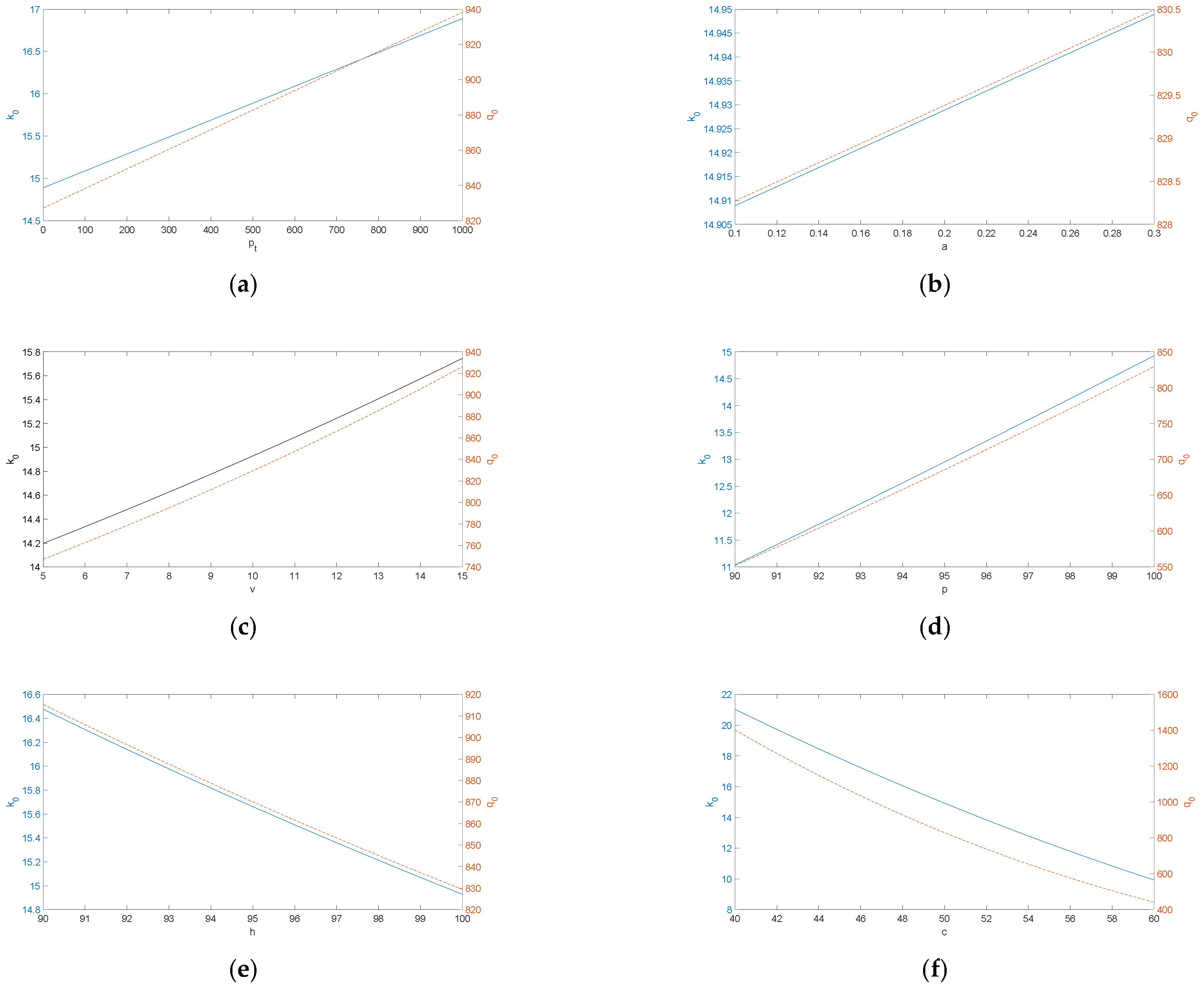
Proposition 1. Under the centralized decision scenario, the optimal product green level isand the optimal order quantity is Under government-regulated carbon quotas, and with increasing consumer awareness of environmental protection, companies can improve the overall profitability of their supply chain, by making centralized decisions, to enhance the eco-friendliness of their products. The product green level and the order quantity are jointly concave. We found that the optimal product green level and the optimal order quantity are affected by the other parameters, such as retail price, salvage value, R&D cost coefficient, etc. Then, we conducted a sensitivity analysis, and obtained the following proposition.
Proposition 2. Both and increase in , a, v and p, but decrease in h and c.
As retail price
p or salvage value
v increases, the goods are more profitable from sales, or lose less from salvage, so both the optimal product green level and the optimal order quantity should be increased, to advance the probability of goods sales (see
Figure 1c,d); however, as the total unit cost
c decreases, the profitability of goods is decreased, such that both the optimal product green level and the optimal order quantity should be decreased, to avoid the loss from salvage (see
Figure 1f). As emission reduction efficiency coefficient
a or carbon trading price
increases, the product green level can be increased, to improve the supply chain’s revenue; however, as the R&D cost coefficient of product green level
h increases, the product green level should be decreased, to reduce the supply chain’s cost. As the optimal order quantity increases in the optimal product green level, then the optimal order quantity increases in emission reduction efficiency coefficient
a or carbon trading price
(see
Figure 1a,b), but decreases in the R&D cost coefficient of the product green level (see
Figure 1e).
3.3. Decentralized Decision Model under the Buyback Contract
Under a buyback contract with the green product
cost-sharing, the retailer helps the green product manufacturer bear part of the research and development costs at a ratio of
, while the green product manufacturer bears a proportion of
. The manufacturer and retailer reach an agreement in advance that the retailer can obtain products from the manufacturer at a wholesale price
w. At the end of the sales period, the manufacturer will compensate for unsold products at a repurchase price
b. However, as transportation of remaining products also incurs costs, these products will not be shipped back to the manufacturer, and their residual value still belongs to the retailer. In the green supply chain buyback model, the expected profit functions for retailers and green product manufacturers are
and
, respectively:
Proposition 3. Under the decentralized decision scenario, there is an equilibrium between the manufacturer and the retailer; the equilibrium green level of products isand the equilibrium order quantity is Under the decentralized decision scenario, the manufacturer and the retailer make their own decisions in relation to the green level of products and product order quantity. We obtain a unique equilibrium, in which both the green level of products and the order quantity are affected by other parameters, such as retail price, salvage value, cost coefficient, etc. Then, we conduct a sensitivity analysis under the decentralized decision scenario, and obtain the following proposition.
Proposition 4. Both and increase in , a, v, b and p, but decrease in h, θ and .
Under the decentralized decision scenario, in equilibrium, as retail price p or salvage value v increases, the goods are more profitable from sales, or lose less from salvage, so both the equilibrium product green level and the equilibrium order quantity should be increased, to advance the probability of goods sales. However, as the unit marginal cost increases, the profitability of goods is decreased, such that both the equilibrium product green level and the equilibrium order quantity should be decreased, to avoid the loss from salvage. As emission reduction efficiency coefficient a or carbon trading price increases, the product green level can be increased, to improve the product’s revenue, so as to increase the product’s profit. However, as the cost coefficient of product green level h increases, the product green level should be decreased to reduce the supply chain’s cost. As the product’s proportion of the cost increases, a lower equilibrium product green level should be set, to retain its profit. As the equilibrium order quantity increases in the equilibrium product green level, then the equilibrium order quantity increases in emission reduction efficiency coefficient a or carbon trading price , but decreases in the cost coefficient of product green level and the product’s proportion of the cost.
4. Coordination under the Buyback Contract
In the centralized system, the supplier and the retailer are considered as a whole part, and maximize the channel profit by deciding q and k, which are the global optimal decisions for the supply chain. However, in the decentralized system, the supplier and the retailer maximize their own profit such that the optimal decision q and k are local optimal, not global optimal. Consequently, the local optimal profit is lower than or equal to the global optimal profit. With the coordination mechanism in this part, the local optimal profit equals the global optimal profit.
In research on coordinating supply chain systems through the buyback contract, many studies have found that in the real world, the buyback contract can indeed help participants at all levels of the supply chain to effectively enhance their optimal interests. The buyback contract has gradually become one of the measures by which suppliers and retailers can expand sales volume: on the one hand, it promotes further cooperation between the manufacturer and the retailer, and encourages both parties to make decisions from the perspective of maximizing the benefits of the supply chain system; on the other hand, it is conducive to increasing the benefits of the green product retailer and manufacturer, and to improving system performance [
31].
When the retailer’s order quantity decision is the same as the previous centralized decision, and the manufacturer’s product eco-friendliness is the same as the centralized decision, the green supply chain reaches coordination, and should satisfy the conditions: , .
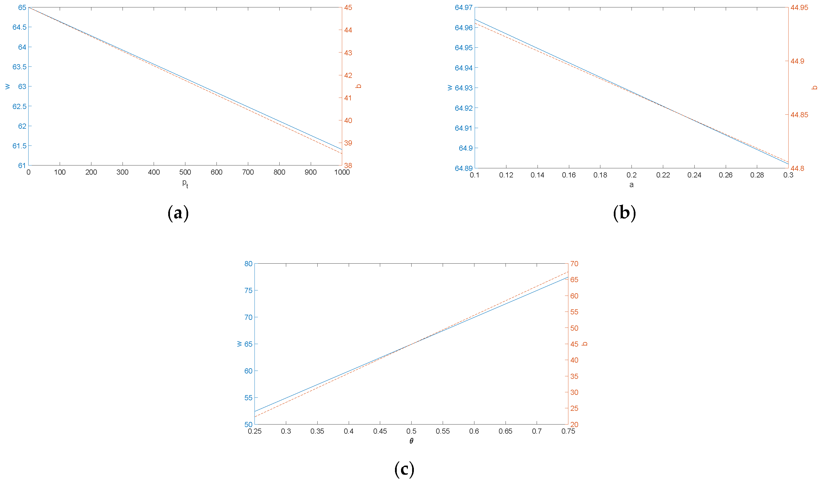
Proposition 5. For a contract combining buybacks and research and development cost-sharing to achieve perfect coordination of the system, the following parameters must meet the conditions: Under the contract, the manufacturer and the retailer share the risk of demand uncertainty by the cost share of the and buyback behavior from the manufacturer to the retailer. Specifically, the retailer bears of the manufacturer’s research and development costs, the manufacturer compensates the retailer for unsold products at a repurchase price b at the end of the sales period, and the supply chain is coordinated. The wholesale price and buyback price are both affected by other parameters, such as retail price, salvage value, etc. Next, we conducted a sensitivity analysis, and obtained the following proposition.
Proposition 6. When the supply chain is coordinated, w increases in θ, but decreases in and a; b increases in θ, but decreases in and a.
As emission reduction efficiency coefficient
a or carbon trading price
increases, the product green level can be increased to improve the product’s revenue, so as to increase the product’s profit. As the equilibrium order quantity increases in the equilibrium product green level, then the equilibrium order quantity and channel optimal order quantity increases in emission reduction efficiency coefficient
a or carbon trading price
. However, due to the
cost sharing between the manufacturer and the retailer, the equilibrium order quantity increases more, such that the buyback price needs to be reduced, to slow the equilibrium order quantity increment range, so as to remain consistent with the optimal order quantity. As the manufacturer’s proposition of the
cost
increases, the equilibrium order quantity’s increment is close to the channel optimal order quantity’s increment, such that the motivation of the buyback price decrement is diminished. As the wholesale price increases in the buyback price, then the wholesale price increases in the manufacturer’s proposition of the
cost (see
Figure 2c), but decreases in the emission reduction efficiency coefficient or carbon trading price (see
Figure 2a,b).
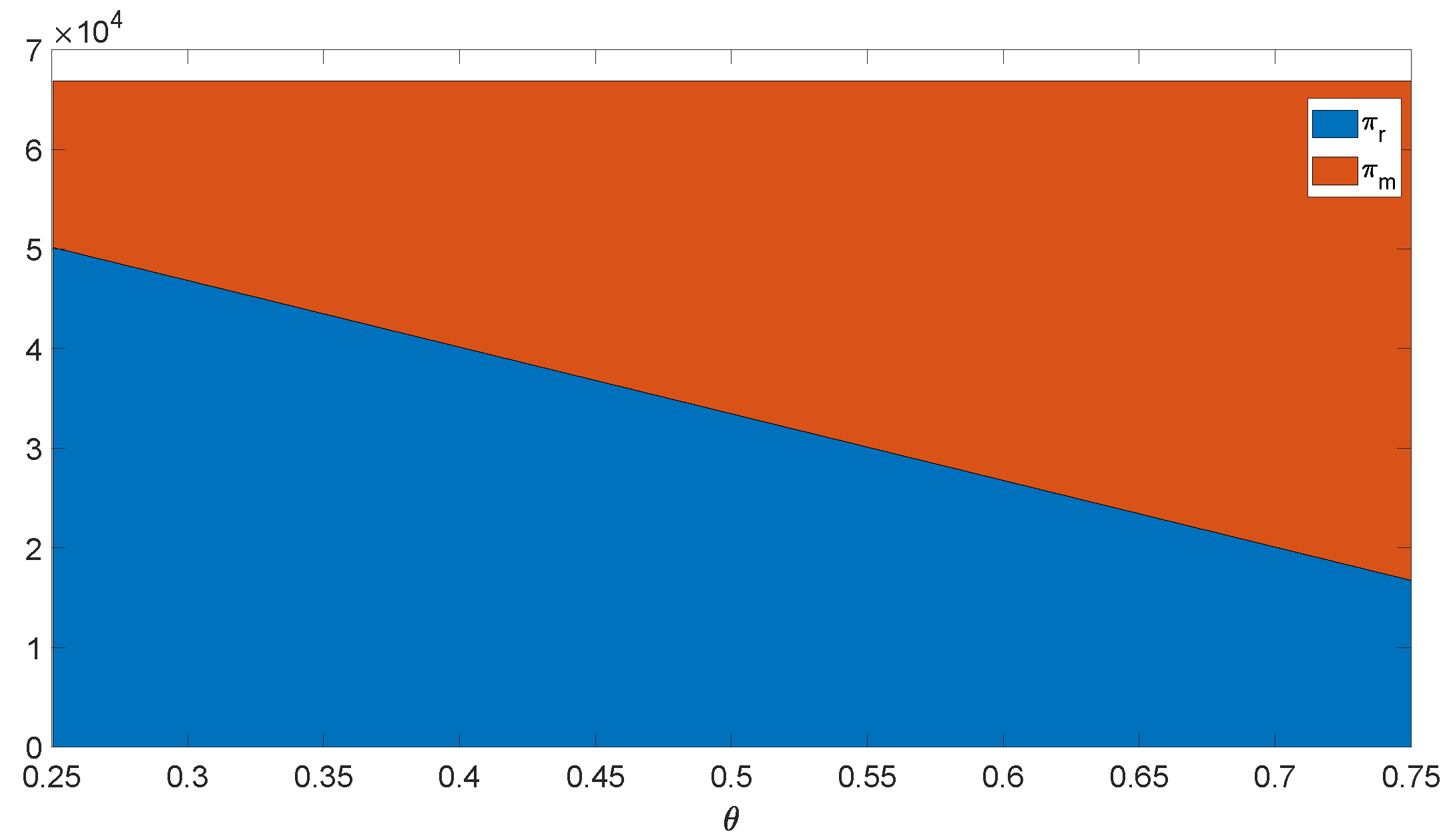
With the wholesale price and buyback price, the supply chain can be coordinated, and the supply chain profit can be maximized. Due to the cost sharing between the manufacturer and the retailer, can be used to distribute the total optimal supply chain to the manufacturer and the retailer.
In decentralized decision-making, the green product manufacturer decides the optimal product green level
k, and the retailer decides the optimal order quantity
q on this basis. When the supply chain is coordinated, due to the
cost sharing between the manufacturer and the retailer,
can be used to distribute the total optimal supply chain between the manufacturer and the retailer. As
increases, the changes in profits of all parties are shown in
Figure 3. Under the buyback and
cost-sharing contract, when
, the retailer’s profit is 50,150; the green manufacturer’s profit is 16,697 when the supply chain is coordinated, and the channel profit is 66,848. As
increases, the retailer profit decreases but the manufacturer increases, and the channel profit is unchanged. Therefore, the
cost sharing,
, can be used to distribute the optimal channel supply chain between the manufacturer and the retailer.
5. Sensitivity Analysis on the Optimal Channel Profit
With the channel optimal product green level and the channel optimal order quantity, the optimal channel profit is
where
.
Next, we analyzed the impacts of parameters on the optimal channel profit, and obtained the following proposition.
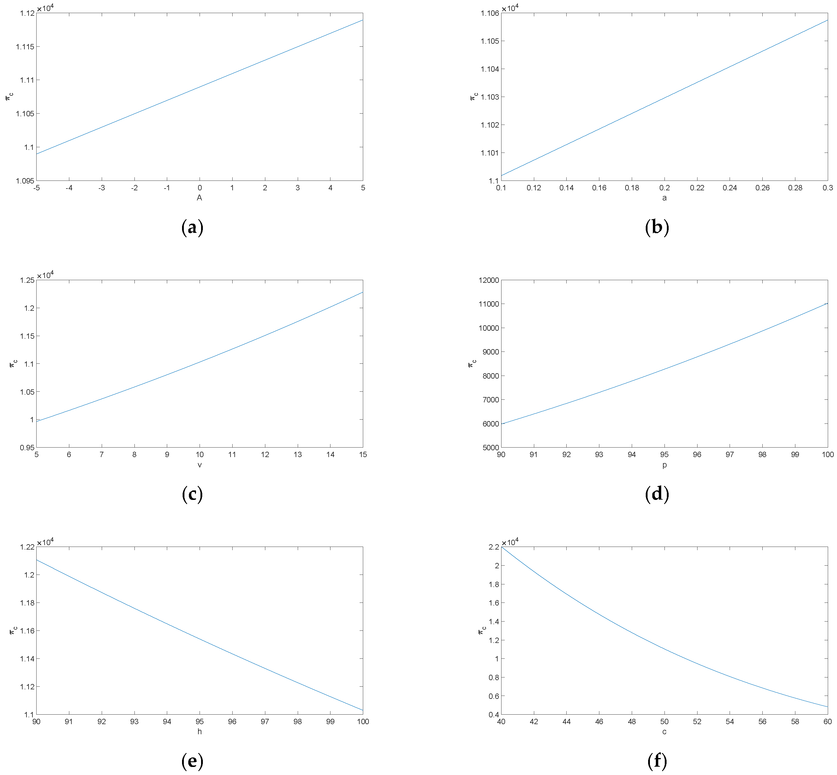
Proposition 7. The channel profit increases in a, p, v and A, but decreases in c and h.
As retail price
p or salvage value
v increases, the goods are more profitable from sales, or lose less from salvage, so the channel profit is increased (see
Figure 4c,d). However, as the total unit cost
c or
cost coefficient
h decreases, the profitability of goods is decreased, such that the channel profit is decreased (see
Figure 4e,f). As the normal product carbon emission trading
A or emission reduction efficiency coefficient
a increases, the manufacturer can obtain more profit from the product carbon emission trading, such that the channel profit is increased (see
Figure 4a,b).
The increment of
always leads to the increment of the optimal product green level
and the optimal order quantity
. If the carbon trading price
is low (
), the manufacturer will set a low product green level, and the product carbon emission trading is a cost for the supply chain (
). The increment of
leads to a higher cost, such that the channel profit
is decreased; however, if the carbon trading price
is high (
), the manufacturer will set a high product green level, and the product carbon emission trading is a revenue for the supply chain (
). The increment of
leads to a higher revenue, such that the channel profit
is increased (see
Figure 5).
Proposition 8. The channel profit decreases in when , but increases in when , where .
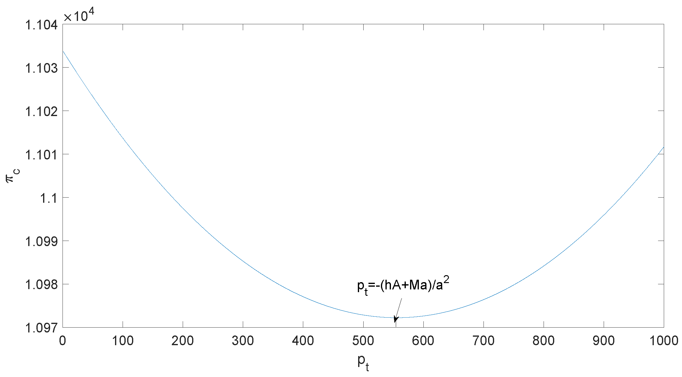
Whether the product carbon emission trading is a revenue or a cost for the green supply chain depends on the threshold of the carbon trading price . We then analyzed the impact of the parameters on the threshold of the carbon trading price , and obtained the following proposition.
Proposition 9. The threshold decreases in A, p and v, but increases in c and h. when , the threshold decreases in a; when , is negative, and always holds.
Whether the product carbon emission trading is a revenue or a cost for the green supply chain depends on the threshold of the carbon trading price . Consequently, when increases, it is more probable that , and the product carbon emission trading will be a cost for the supply chain; when decreases, it is more probable that , and the product carbon emission trading will be a revenue for the supply chain.
The increment of the retail price p or salvage value v leads to a higher product green level , so it is more probable that carbon emission trading will be a revenue; however, the increment of the total unit cost c leads to a lower product green level , so it is more probable that carbon emission trading will be a cost.
The increment of the cost h always leads to a higher product green level , so it is more probable that carbon emission trading will be a revenue. As the normal product carbon emission trading A increases, the product green level remains unchanged, but it is more probable that the product carbon emission trading will be a revenue () for the supply chain, such that decreases.
When the emission reduction efficiency coefficient a is low (), is low, such that the product carbon emission trading is a cost for the supply chain; therefore, the increment of a leads to the increment of , such that the product carbon emission trading becomes the revenue for the supply chain, and it is more possible that . When the emission reduction efficiency coefficient a is high enough (), is high, such that the product carbon emission trading is a revenue for the supply chain, and always holds.
6. Conclusions and Further Research
6.1. Conclusions
Unlike the traditional buyback contract, under the green supply chain buyback contract, both the product green level and order quantity need to be decided, and the product green level is related to the random demand. In addition, the cost is shared between the manufacturer and the retailer. In order to coordinate the green supply chain, the manufacturer needs to share both the risk of goods salvage and the cost.
Under the green supply chain buyback contract, we find that both the wholesale price and buyback price increase in the manufacturer’s proposition of the cost, but decrease in the emission reduction efficiency coefficient or carbon trading price.
As retail price increases or as salvage value increases, the goods are more profitable from sales, or lose less from salvage, so both the optimal product green level and the optimal order quantity should be increased, to advance the probability of goods sales, such that the channel profit is increased. However, as the total unit cost increases, the profitability of goods is decreased, such that both the optimal product green level and the optimal order quantity should be decreased, to avoid loss from salvage, such that the channel profit is decreased.
As the emission reduction efficiency coefficient increases, the product green level can be increased, to improve the supply chain’s revenue, so as to increase the supply chain profit; however, as the cost coefficient of the product green level increases, the product green level should be decreased, to reduce the supply chain’s cost. As the optimal order quantity increases in the optimal product green level, then the optimal order quantity increases in the emission reduction efficiency coefficient, but decreases in the cost coefficient of the product green level. The channel profit increases in the emission reduction efficiency coefficient, but decreases in the cost coefficient of the product green level.
As the carbon trading price increases, the product green level can be increased, to improve the supply chain’s revenue, so as to increase the supply chain profit. As the optimal order quantity increases in the optimal product green level, then the optimal order quantity increases in the carbon trading price. If the carbon trading price is low, the manufacturer will set a low product green level, and the product carbon emission trading will be a cost for the supply chain. The increment of the carbon trading price leads to a higher cost, such that the channel profit is decreased; however, if the carbon trading price is high, the manufacturer will set a high product green level, and the product carbon emission trading will be a revenue for the supply chain. The increment of the carbon trading price leads to a higher revenue, such that the channel profit is increased.
6.2. Further Research
For the convenience of research and modeling, this paper simplified the actual situation of the supply chain. This has resulted in a certain degree of deviation between the research results and the actual situation. The main shortcomings are as follows. The relationship between members of the supply chain is complex and changeable, so it is not appropriate to discuss them together: on the one hand, there is not much attention paid to the quantitative relationship between buyers and suppliers; on the other hand, whether there is competition or cooperation between suppliers has not been considered. In reality, game behavior often occurs under conditions where information among members of the supply chain is not equal, and decision-making is not completely rational. This study assumes that product greenness and consumer purchase preferences are not completely positively correlated: that is, consumers do not completely pursue green consumption.
Under the current premise of carbon emissions, the exploration of green supply chain repurchase contracts can be extended to the following areas.
Firstly, green supply chain coordination can also be studied in multiple suppliers and multiple stages of products. At present, most repurchase contract explorations are basically focused on the coordination between a single cycle, a single product and a single retailer. However, in practice, the structure of the supply chain involved in practical life is much more complicated than in theory; therefore, it would be possible to consider further expanding the exploration of repurchase contracts involved in green supply chains to one-to-many or many-to-one modes between supply chains and retailers. The exploration could even be further expanded to multi-cycle, multi-level and multi-product type supply chain network structures.
Secondly, during the period when productivity constraints arise in green supply chains. At present, the exploration of green supply chain repurchase contracts is based on the assumption that the production and supply capacity of manufacturers or suppliers is infinite. There is scant related literature that considers situations where the production capacity of manufacturers is limited; however, in practice, most enterprises have significant constraints on their production capacity; therefore, in actual operation, how to reasonably arrange the production capacity of suppliers or manufacturers, so as to effectively improve their own resource utilization rate, has become a major concern for most enterprises.
The issue of information asymmetry in green supply chains is also a difficult problem that we need to carefully consider. In cooperation, due to asymmetric information, coordination mechanisms may not be able to enable both supply and demand sides to make global optimal decisions, resulting in the reduction of supply chain profit; therefore, in future, some treaties and parameters could be set to associate with some effective information. Of course, the ultimate goal is to make the upstream and downstream information of the green supply chain fully flow, and to further improve the overall collaborative efficiency.


