Roadmap Optimization: Multi-Annual Project Portfolio Selection Method

Abstract

The process of project portfolio selection is crucial in many organizations, especially R&D organizations. There is a need to make informed decisions on the investment in various projects or lack thereof. As the projects may continue over more than 1 year, and as there are connections between various projects, there is a need to not only decide which project to invest in but also when to invest. Since future benefits from projects are to be depreciated in comparison with near-future ones, and due to the interdependency among projects, the question of allocating the limited resources becomes quite complex. This research provides a novel heuristic method for allocating the limited resources over multi-annual planning horizons and examines its results in comparison with an exact branch and bound solution and various heuristic ones. This paper culminates with an efficient tool that can provide both practical and academic benefits.

1. Introduction

Most project-based organizations are faced with a long list of proposed projects that compete for a limited set of resources such as money, manpower, and equipment [1]. Project portfolio selection (PPS) aims to find which projects an organization should take [2,3,4]. Needless to say, as the decision to allocate and prioritize projects today affects the organization’s competitive position in the future [5], and the decisions of initiation (and termination) of projects are of a strategic nature since they involve the commitment of substantial enterprise resources [6], it is recognized worldwide that there is a need to manage projects as an overall portfolio [7] and not as separated projects [8].

Evidently, organizations wish to maximize their return on investment when selecting projects [9], and therefore, the selection process should be based on criteria that take into account this objective function [10].

The operational research problem of PPS was defined [11] as the situation where several projects are available for investment. They are different in their resource needs (both resource types and resource demand level).

The current research and method are lacking in two aspects: they do not take into consideration the time value of the projects (i.e., contribution depending on the projects’ completion time), and they also do not consider the dependence between the projects (i.e., precedence and competition over resources). This research aims to present a novel formulation of the problem, namely one that incorporates theses aspects. The article also provides an exact solution algorithm (branch and bound) that can solve small to medium problems. However, due to the NP-hard nature of the problem, large-scale problems require a different approach. Thus, several metaheuristic algorithms are proposed and analyzed.

2. Literature

The research in the area of project portfolio selection has been growing intensively in the past decade, with intensive proliferation of research articles tackling a myriad of variations of this problem. Some of this proliferation was summarized in several review papers. For example, Frey and Buxmann [12] reviewed the literature on portfolio selection of IT projects. Weissenberger-Eibl and Teufel [13] provided a strategic and political review on project selection. Padhy [14] and Condé and Martens [15] reviewed six-sigma project selections. Danesh et al. [16] provided a broad review of multi-criteria portfolio management, and Mohagheghi et al. [17] reviewed models, uncertainty approaches, solution techniques, and case studies.

The simplest model of the project selection problems is single-attribute optimization under resource constraints. This problem resembles the well-known knapsack algorithm [18,19]. This problem was primarily extended to reflect synergies and uncertainty [18]. The main extensions to this type of optimization were with interactions and under uncertainty [20,21].

Another classical model of the project selection problem is financial project portfolio selection, which is based on mean profit vs. profit variance [22]. However, this model of portfolio selection is rooted in investment in the stock markets, and its use is indeed more suited to investment decisions in a portfolio of stocks and other financial assets. Thus, only a few papers on project portfolio selection adopted this modeling approach [9]. This model’s assumptions and characteristics are more suited to pure investment decisions than to a company or organization decision problem.

Biobjective models were a natural evolution of single-objective optimization [20,23]. While multi-objective optimization became the research mainstay of project portfolio selection, biobjective models, due to their simplicity, still attract some research attention [19,23,24,25].

The multi-objective optimization models followed the aforementioned models [26,27,28,29,30]. The literature on multi-objective project portfolio selections proliferated [31,32,33,34,35,36] and became the main branch of the project portfolio research [16], and it is still prevalent [37]. Within this multi-objective framework, robustness became a prevalent requirement and an objective to address the uncertainties of project portfolio selection [29,32].

During the last two decades, fuzzy logic started to play an important role in decision making, and in the past decade, it made its way into the portfolio selection literature. For example, Perez and Gomez [33] and Perez et al. [38] used fuzzy constraints between projects, while others [1,35,39,40] used them in the objective function.

Another branch of research gathered both project scheduling and project selection into a single decision frame (some examples are in [19,30,41,42,43]).

While the above discussion dealt with project selection in technical terms, strategic project portfolio selection presents a very different approach [25,44,45,46]. Killen et al. [4] identify three strategic perspectives of project portfolio selection: (1) the resource-based view, (2) the dynamic capabilities view, and (3) the absorptive capacity view. Kaiser et al. [47] stressed the role of structural alignment of selected projects with the organization’s values, vision, and strategy. Kopmann et al. [46] suggested fostering both deliberate and emergent strategies. Finally, Guo et al. [25] suggested balancing strategic contributions and financial returns.

While the existing reviews cover their relevant part of the literature and suggest some classifications of the project selection problems, a more formal and general classification system can contribute to them. We suggest a system that would be close to Kendall’s notation in queuing theory [48]. To foster a discussion for filling this gap, we present here our initial attempt at classification of project portfolio selection’s main problem types using the major characteristics of these problems. It is hoped that the suggested classification scheme will initiate a discussion (or even a debate) which will culminate in an agreed-upon standard classification method. In Figure 1, we propose a classification method for the PPS problem. The suggestion is to classify the problems by their objective type, the solution method used to make the selection, the nature of the data, and the constraints. Therefore, the proposed method has four classifiers:

X—

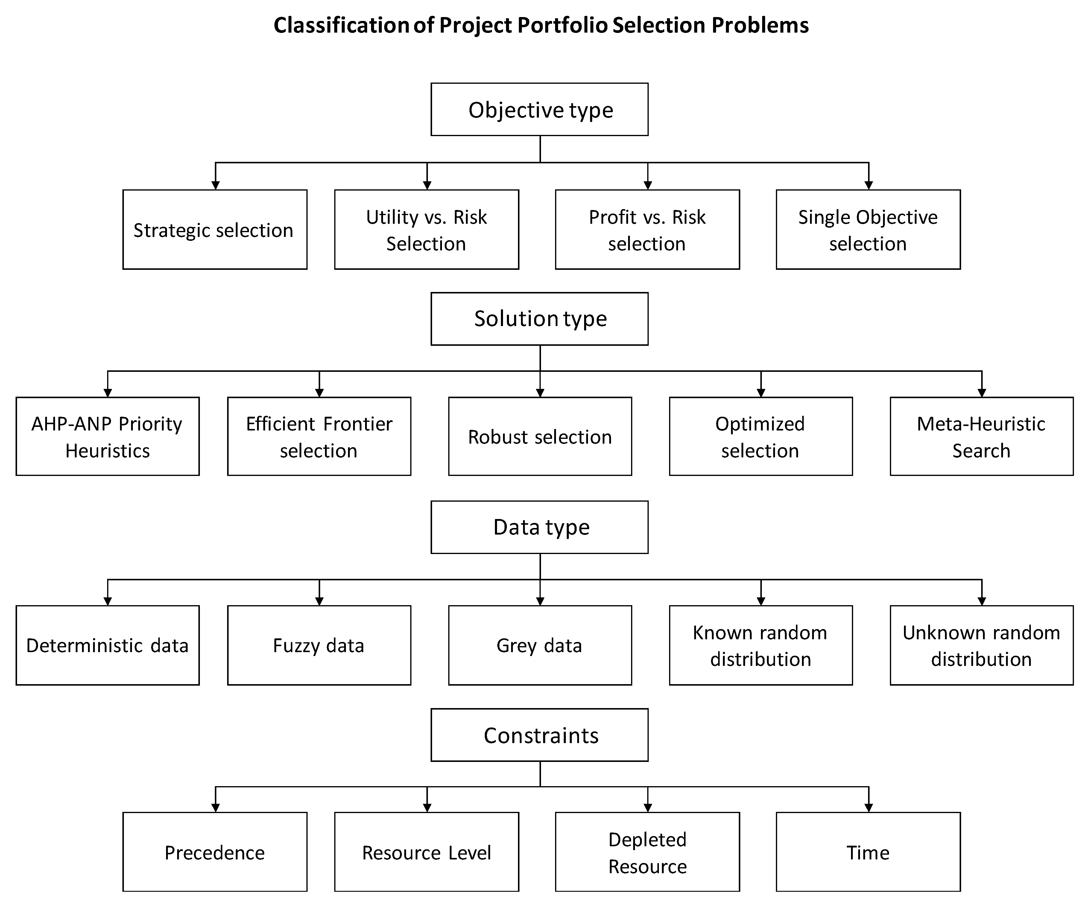
Objective type: single-attribute selection, multiple-attribute selection, fitness function, profit vs. risk selection, utility vs risk selection, and strategic selection;

Y—

Solution type: optimized selection, robust selection, efficient frontier, AHP/ANP, and priority-based;

Z—

Data type: deterministic data, fuzzy data, and stochastic data;

W—

Constraint characteristics: a combination of letters that testify for the existence of the characteristic constraint as follows: P = precedence constraints, RL = resource-level constraints, DR = depleted resource constraints, and T = time constraints.

Some examples of this classification scheme are shown in

Table 1. Examples of the suggested classifications.

	Reference	Objective Type	Solution Type	Data Type	Constraints Combination
1	[33]	Multi-objective	Efficient frontier	Fuzzy	P, RL, DR, T
2	[49]	Strategic selection	None	Deterministic	P, RL, DR, T
3	[50]	Single-objective selection	Optimized	Deterministic	P, RL, DR, T
4	[51]	Single-objective selection	Optimized	Deterministic	P, RL, DR, T
5	[52]	Single-objective selection	Optimized	Known random distribution	P, RL, DR, T
6	[53]	Profit vs. risk selection	Optimized	Known random distribution	None
7	[32]	Multi-objective	Robust selection	Deterministic	P, RL, DR, T

.

As stated above, enhancements to this classification scheme and even challenges are welcome as part of future research.

The problem researched in this article is of a single objective (maximum value); the data are assumed to be deterministic, and no depleted resources are concerned. The article utilizes two solution types: optimal for small-to-medium-sized problems and metaheuristic searching for larger ones. Therefore, this problem should be classified according to the hierarchical classification of Figure 1 as multi-attribute, optimized, and deterministic.

This article does not consider random, fuzzy, or gray data.

3. Problem Description

The problem deals with an ongoing situation of R&D to develop projects. The need is to decide which projects should be scheduled for each year in the planning horizon. As a company has a limited amount of resources each year, it is impossible to perform all projects at once, and therefore, there is a need to schedule less-lucrative projects for distant years. In the case of no constraints, all projects would have been planned for the first year. However, this is not the case. Two reasons compel postponing projects to future years:

• Resource availability: Each project requires a specific level of various resources. The assumption is that there cannot be a breach of the available level of each resource.
• Precedence: As part of the R&D project, the company acquires new capabilities that can be exploited for future projects.

3.1. Problem Assumptions

• Each project has a specific value to the company. This value can be measured in the same units (typically profit, measured in dollars).
• The value of the project to the company depreciates as a function of time; that is, each year can be assigned a corresponding coefficient that expresses the depreciated value. (For example, a project assigned to year 1 has a value of 100. The same project assigned to year 2 has a value of 80. If assigned to year 3, it has an even lower value, etc.).
• All relevant resources are renewable (e.g., work hours). For each year, there are new levels of resources available. The amount of a resource that was not consumed in year n cannot be used in year n + 1.
• Each project has given levels of resources needed for its completion (e.g., programmer hours or QA hours).
• Technical precedence dependencies exist between the projects. Thus, project x can be performed based on the technology performed for project y.

3.2. Problem Notations

To assist understanding of the formulation,

Table 2. Problem notations.

Notation	Definition
$\overline{\mathcal{Y}}$	A vector of all the depreciation values of the years. $y_i\in \overline{\mathcal{Y}}$ is the value of year $i$.
$\stackrel{=}{ℛ}$	A matrix containing the available resources at each year in the planning horizon. $r_{j,i}\in \stackrel{=}{ℛ}$ is the level of resource $j$ at year $i$.
$\stackrel{=}{\mathcal{Q}}$	A matrix containing the required resources for each project. $q_{k,j}\in \stackrel{=}{\mathcal{Q}}$ is the requirement of resource $j$ of project $k$.
$\overline{\mathcal{P}}$	A vector of all the contributions (values) of the projects. $p_k\in \overline{\mathcal{P}}$ is the value of project $k$.
$\stackrel{=}{\mathcal{D}}$	A matrix containing technical dependencies. $d_{k,m}\in \stackrel{=}{\mathcal{D}}$ has the following values:       $d_{k,m}=\{\begin{array}{cc}1& if project m depends on project k\\ 0& otherwise\end{array}$
$\stackrel{=}{\mathcal{X}}$	Decision variable matrix. $x_{k,i}\in \stackrel{=}{\mathcal{X}}$ has the following values:        $x_{k,i}=\{\begin{array}{cc}1& if project k is to be completed in year i\\ 0& otherwise\end{array}$
$\mathcal{V}$	Total portfolio value.
$\stackrel{=}{Z}$	Auxiliary variables, denoting the years the project is in process.
$\stackrel{=}{\mathcal{W}}$	Auxiliary decision variables denoting the level of resources used by a project in any given year.
$N$	Number of projects in the examined portfolio.
$H$	Planning horizon (number of years).
R	Number of resource types.
$\overline{G}$	Genotype vector.
$i,j,k,l,m,n$	Indices: $i,l$—Year index. $j$—Resource index. $k,m,n,p$—Project index.

depicts the notations used for the formulation.

3.3. Problem Formulation

The objective function is for maximizing the cumulative value of the project portfolio such that

$$max\mathcal{V}=\sum _{\forall y_i\in \overline{\mathcal{Y}}}\sum _{\forall p_k\in \overline{\mathcal{P}}}\sum _{\forall x_{k,i}\in \stackrel{=}{\mathcal{D}}}{y}_i{p}_k{x}_{k,i}$$

(1)

Each project is to end in one year only, so the relevant constraints are

$${{\displaystyle \sum }}_{\forall i}{x}_{k,i}=1 \forall k\in \left\{1,2,\dots ,N\right\}$$

(2)

Since a project can stretch over more than one year (i.e., start before its final year), there is a need for an auxiliary set of variables ($\stackrel{=}{Z}$), denoting the years a project can use resources (i.e., the project cannot use resources after its ending):

$$z_{k,i}\le {{\displaystyle \sum }}_{l=i}^H{x}_{k,l} \forall k\in \left\{1,2,\dots ,N\right\}$$

(3)

Thus, $z_{k,i}$ can have the maximum value of 1 for each year until its ending year and 0 onward.

To ensure that the project spreads over consecutive years, we use

$$z_{k,i}\le z_{k,i+1} \forall k\in \left\{1,2,\dots ,N\right\},\forall i\in \left\{1,2,\dots ,H-1\right\}$$

(4)

This notification enables the setting of the resource-consuming variables ($\stackrel{=}{\mathcal{W}}$), denoting the level of resource j consumed by project k at year i:

$$w_{k,i,j}\le q_{k,j}{z}_{k,i} \forall k\in \left\{1,2,\dots ,N\right\}, \forall i\in \left\{1,2,\dots ,H\right\}, \forall j\in \left\{1,2,\dots ,P\right\}$$

(5)

Thus, a project may consume part of the resources it needs in year n and part of year n + 1 (e.g., use 2023’s budget and 2024’s budget). Additionally, each project must consume all the needed resources:

$${{\displaystyle \sum }}_{i=1}^H{w}_{k,i,l}=q_{k,j} \forall k\in \left\{1,2,\dots ,N\right\},\forall l\in \left\{1,2,\dots ,H\right\}$$

(6)

To prevent over-consumption of resources at any given year, the resource level constraints are

$${{\displaystyle \sum }}_{\forall k}{{\displaystyle \sum }}_{\forall i}{w}_{k,j}\le r_{j,i} \forall j\in \left\{1,2,\dots ,P\right\}$$

(7)

Finally, the technical dependencies among the projects are expressed as

$$z_{k,i}\ge z_{m,i} \forall d_{k,m}=1,\forall i\in \left\{1,2,\dots ,H\right\}$$

(8)

A small example to help illustrate this formulation is detailed in the Appendix A.

4. Problem Complexity and Exact Solution

Although the formulation depicted in Section 3.3 is accurate and needed, it is of little contribution when trying to solve such problems. The described problem is NP-complete, yet exact solutions can be obtained via the branch and bound (B&B) method. Section 4.1 describes a B&B solution for this problem.

Since a B&B solution is practical for some of the problems, and the NP-completeness of the general problem hinders exact solutions, a practical and efficient metaheuristic solution is described in Section 5. This solution method is useful for large-sized problems and also provides an initial upper bound for the B&B algorithm.

4.1. Complexity

To prove the NP-completeness of the PPS, a reduction to a well-known problem is needed: the precedence constraint knapsack problem [54]. The reduction is performed as follows:

• Set the horizon (number of years) to 2. Thus, the projects are either assigned to the first year (i.e., inserted to the “knapsack”) or to the second one (left out).
• Set the second year’s value to zero ($y_2=0$).

As PPS is far more complicated than this, it is clear that PPS is of an NP-complete nature.

4.2. Branch and Bound Algorithm

An efficient B&B algorithm is based on the following components:

• A lower bound (LB): Any feasible solution can provide an LB. The algorithm can start with either a solution produced by the metaheuristic algorithm or a simple heuristic solution.
• An upper bound (UB): This is an efficient way to assess the maximal potential of a partial solution (i.e., branch) of the tree. The UB can serve as a convenient heuristic precedence rule (i.e., a rule to decide which branch to further develop first).
• A branching method: This is a way to create the net branches.

The following subsections describe the components of the algorithm.

4.2.1. Initial Solution

It is convenient (though not necessary) to start the run of the algorithm with a lower bound (LB). The higher the LB, the better. A reasonable algorithm should consider all important attributes of the projects, namely the resource requirements and precedence. The following algorithm can provide a decent initial solution:

• For each resource type ($j$):

  1.1

  Calculate for each project the ratio of the project value to its resource requirement; that is, ${\theta }_k=\frac{p_k}{q_{k,j}}$, where ${\theta }_k$ denotes the value that can be obtained from one unit of the resource by performing the project.

  1.2

  For each project, calculate its total impact. The impact is calculated by aggregating the project’s ${\theta }_k$ value and the values of all its successors (direct and indirect). For example, for project 1, the impact is $I_1={\theta }_1+{\theta }_5+{\theta }_7+{\theta }_8$ (since projects 5, 7, and 8 are successors to project 1).

  1.3

  Sort the projects in descending order by the total impact.

  1.4

  Schedule the projects according to the order obtained in Step 1.3. Each project should be scheduled for the first available year.

  1.5

  Calculate the total value obtained from the schedule of Step 1.4 $\left[\mathcal{V}\left(j\right)\right]$.

• The solution is set to be $LB=\underset{\forall j}{\max }\mathcal{V}\left(j\right)$.

4.2.2. Branching

The branching process is quite simple. Each “level” of the tree represents a year. Therefore, the tree depth can only be as deep as the planning horizon.

Each branch is simply a set of projects that fully utilize at least one of the resources available for that year; that is, when branching year $i$, each branch is a set $J$ of all the unscheduled projects that fulfill the following requirements:

• There exists a resource type ($j$) for which

  $${\displaystyle \sum }_{\forall i\in J}{q}_{k,j}\ge r_{i,j}$$

  (9)
• For every subset of $J$, denoted by $J^{-}$ (i.e., $J^{-}\subset J$ and not $J^{-}=J$) and for every resource type ($j$), the following is true:

  $${\displaystyle \sum }_{\forall i\in J^{-}}{q}_{k,j}<r_{i,j}$$

  (10)

The two conditions may look cumbersome, but all they mean is that the set $J$ is a set that exploits one resource to the fullest, and any subset of $J$ can be extended by adding project (s).

4.2.3. Bounding Rule

An efficient bounding rule should satisfy the following demands:

• Simply calculable: The rule should provide the result with a low complexity algorithm (otherwise, it provides no benefit).
• Low UB: To trim the tree as much as possible, the UB should be as low as possible.

The following algorithm provides the two demands. The algorithm is based on two relaxations of the problem: the first is ignoring the precedence constraints, and the second is ignoring the multi-resource nature of the problem (by dealing with one resource at a time).

• For each resource type ($j$), the following should be performed:

  1.1

  Ignore all resource requirements (other than resource $j$) and precedence constraints.

  1.2

  The remaining problem is the multiple knapsacks problem. Solve the problem accordingly.

  1.3

  As the multiple knapsacks problem is an NP-complete problem, when a project is scheduled to start in year $i$ and finish in year $i+1$, calculate the obtained value of the project proportional to the year it was scheduled for.

  1.4

  Calculate the total values of the projects (each according to its year) $UB\left(k\right)$.

• Calculate the overall bound $UB=\underset{\forall k}{\min }UB\left(k\right)$.

The proposed algorithm is quite simple and rapid for small-scale problems.

5. Metaheuristic Search

Although the previous section describes an exact algorithm, it is impractical to apply this algorithm (or any exact algorithm) successfully to large-size problems. The algorithm provided in Section 4.2.1 may prove unsatisfactory for even medium- let alone large-scale problems.

To provide near-optimal solutions, a metaheuristic approach is suggested. The benefit of this approach is that (providing enough runtime) optimality is guaranteed. Since the first conception of metaheuristics, many approaches were suggested. The proposed solution is based on the CLONALG metaheuristics. This search method was developed by de Castro and Van Zuben [55]. This basic method can be applied to various scheduling problems, as long as the following requirements are provided [56]:

• Representation of the solution space (i.e., the “antibodies”);
• An initial set of solutions.
• A procedure to create valid mutations in the antibodies (i.e., mutations creating new solutions that are included in the solution space).

Section 5.1 elaborates on the application of the first requirement to PPS. The second requirement application is provided in Section 5.2. Finally, several different mutation algorithms (third requirement) are detailed in Section 6.

5.1. Vector Representation

Although the formulation provided in Section 3 (and the notations of Table 2) is mathematically accurate, the presentation of the decision variables $\left(\stackrel{=}{\mathcal{X}}\right)$ is impractical for the purposed CLONALG process. The main problem is that most possible instances of $\stackrel{=}{\mathcal{X}}$ are not feasible, either because they represent schedules that violate the dependency constraints or violate the resource constraints. An ideal representation is one in which every possible instance represents a feasible solution. Thus, the mutation process would never yield infeasible solutions. Another requirement is that all feasible solutions can be represented (i.e., the vector representation should spread the entire solution space) so the mutation process will not omit any possible solution.

To achieve this, a vector $\overline{G}$ is introduced. This vector represents the “genotype” of the solution (i.e., it is not the schedule itself), but from each possible instance of $\overline{G}$, a feasible “phenotype” ($\stackrel{=}{\mathcal{X}}$, the solution) can be derived. $\overline{G}$ is a vector of $N$ natural numbers (from 1 to $N$), where $g_k$ is the $k^{th}$ project to be scheduled.

The transformation from $\overline{G}$ to $\stackrel{=}{\mathcal{X}}$ (“genotype to phenotype translation”) is performed as follows:

MAIN

• For $k=1$ to $N$, do the following:

  1.1

  If ${\displaystyle \sum }_{j=1}^N{x}_{k,j}=0$ (i.e., $g_k$ has not been scheduled yet):

  Run procedure “FindYear” with parameter $k$.

  1.2

  If ${\displaystyle \sum }_{i=1}^N{x}_{k,j}=1$ (i.e., $g_k$ has already been scheduled):

  Continue.

FindYear($k$)

• For $m=1$ to $k-1$, do the following (without loss of generality, as it is assumed that if project $k$ depends on project $m$, then $k>m$):

  1.1

  If $d_{m,k}=1$ and ${\displaystyle \sum }_{j=1}^N{x}_{m,j}=0$ (project $k$ depends on project $m$, and project $m$ has not been scheduled), run procedure “SCHEDULE” with parameter $m$.

  1.2

  Otherwlse (either project $k$ does not depend on project $m$ or project $m$ has already been scheduled), continue.

• Find the first year $i$ in which $g_k$ can be scheduled (has enough available resources and does not violate dependencies), and set $x_{k,i}=1$.
• Return

This simple algorithm provides the two requirements: (1) any genotype $\overline{G}$ can be converted to a feasible “phenotype” (feasible $\stackrel{=}{\mathcal{X}}$) through a simple process, and (2) all feasible solutions can be originated from a genotype $\overline{G}$.

5.2. Initial Solution Generation

Since the aforementioned procedure makes any vector containing the natural numbers from 1 to $N$ to be a feasible representation of a solution, a procedure to generate an initial feasible solution is quite straightforward; any “scrambled” vector containing the numbers from 1 to $N$ in random order will suffice. To achieve a set of these scrambled vectors, the following method was applied:

• A matrix $\stackrel{=}{\mathcal{S}}$ with dimensions $N\times 2$ was created;
• For i = 1 to $N$ do the following:

  2.1

  Set $s_{i,1}=i$.

  2.2

  Set $s_{i,2}=U\left(0,1\right)$ (random number from the unit uniform distribution).

After this stage, the first column is filled with running numbers and the second with random numbers.

3

Sort $\stackrel{=}{\mathcal{S}}$ in ascending order according to the second column.

4

The first column of $\stackrel{=}{\mathcal{S}}$ is an initial solution vector ($\overline{G}$).

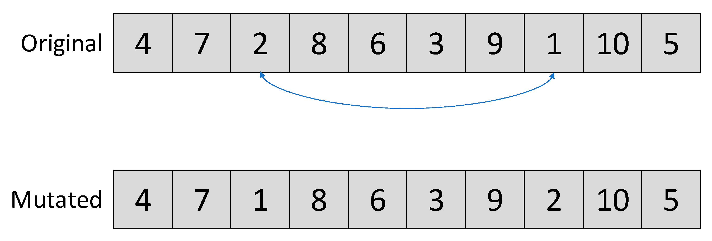
6. Mutation Generation

The presentation of the solution vector and the initial solution set generating set the ground for the central part of the CLONALG process: mutation generation and cloning. The mutations are generated by random change insertion to the genome vector ($\overline{G}$). Since the genotype vector describes the order of scheduling the projects, the mutation process will be carried out by changing this order. This section describes three approaches to the mutation process. The first and the second are “traditional” approaches, and the third one attempts to exploit clustering techniques to improve the search performance. An additional approach is also presented: a combination of the previous ones.

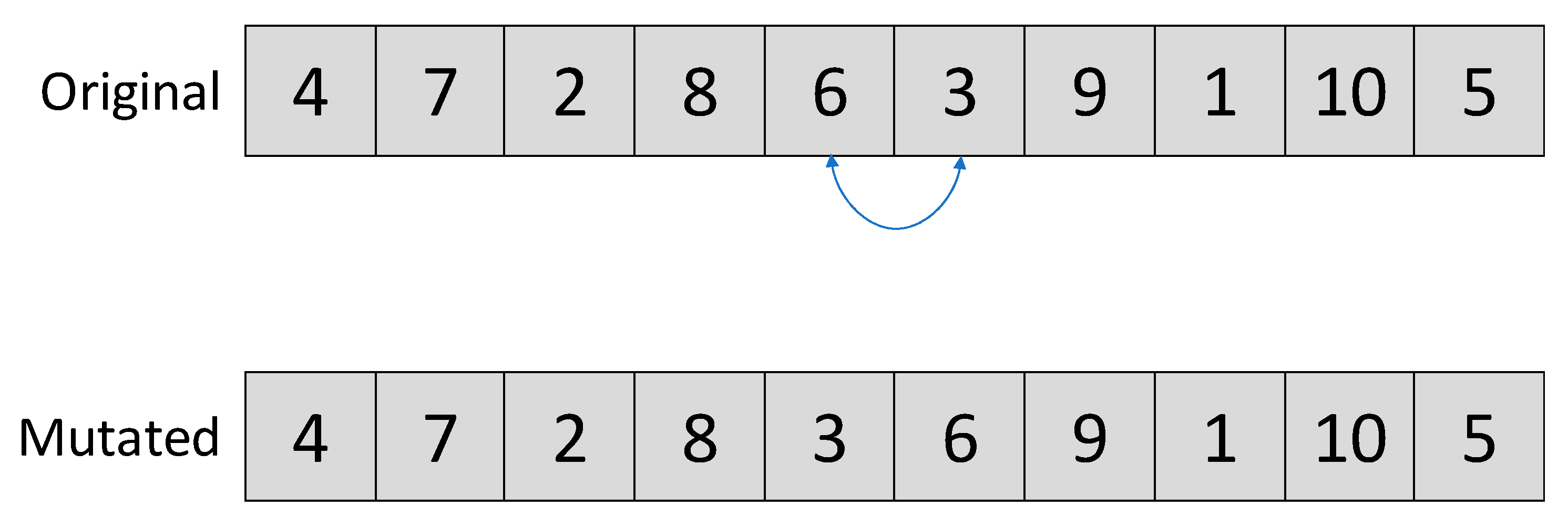
6.1. Minor Mutations

The most trivial and straightforward approach to changing the order of the vector members is by replacement. The simplest way is to randomly choose a project (member of the genotype vector) and replace it with its neighbor, as depicted in Figure 2. In this case, the fifth location (project 6) was chosen and replaced with its neighbor in the sixth location (project 3).

There is an advantage in small mutations. When in the vicinity of the optimal solution, a small mutation is less likely to cause damage and drift away from the optimal solution, as visualized in Figure 3. The small mutation, though in a wrong direction, is less likely to corrupt the solution value than the larger mutation in the correct direction.

6.2. Major Mutations

Though the minor mutations have the advantage of minimal damage when in the vicinity of the optimum, they are likely to provide only minimal improvement (i.e., many steps needed toward the optimum). To illustrate this, let us examine the case depicted in Figure 4.

Project 7 has a high value and therefore should be scheduled ASAP. Let us assume a pre-mutated solution vector $\overline{G}=\left(4,10,1,2,3,5,6,7,8,9\right)$. A mutation switching Projects 1 and 10 may decrease the total value (as Project 10 is postponed) without expediting the lucrative Project 7. This mutation has a high probability of being rejected (decrease in the objective function). To expedite Project 7, there is a need for several “lucky” small mutations. This sequence of small mutations will indeed appear eventually but may take quite a long time. Figure 5 visually depicts the difference between the mutation types.

To improve this, another version of mutations is suggested: randomly choosing two projects in the vector and switching their locations, as depicted in Figure 6. In this case, the third location (Project 2) and the eighth location (Project 1) were switched.

While this “mega-mutation” may prove lethal (i.e., significantly reduce the objective function value), it may also save the need for a lucky sequence of minor mutations.

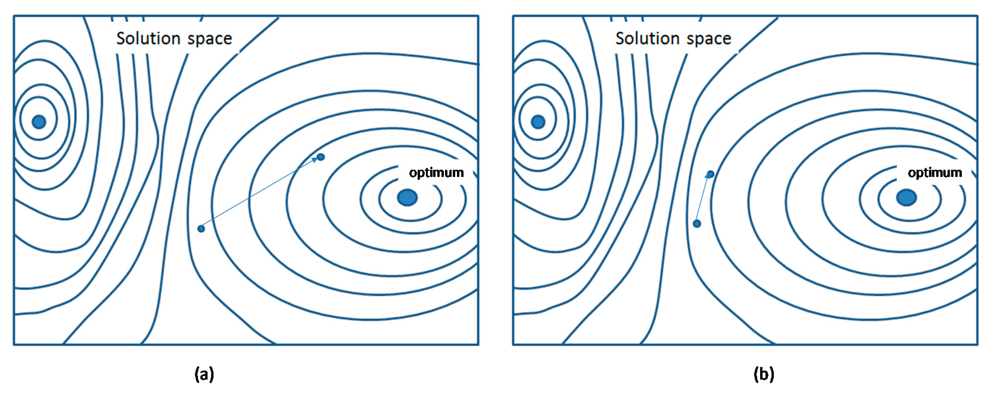
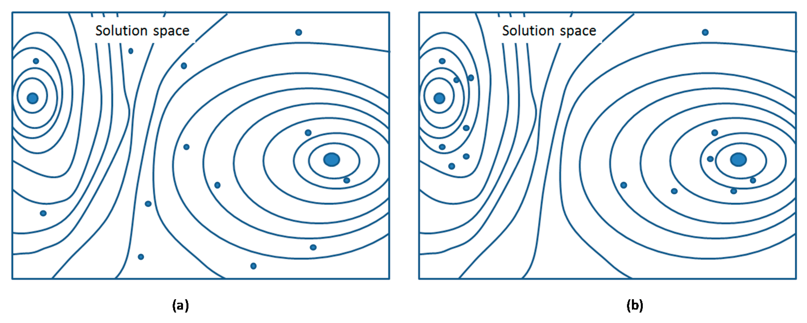
6.3. Oriented Mutations

As claimed by Darwin, in nature, all mutations, whether large or small, are totally random and have no special direction (unlike the Lamarckism theory, which claims that they evolve toward a defined goal). The two mutation types described in Section 6.1 and Section 6.2 are Darwinian; that is, they are totally random, and each project has the same probability to be selected. This full randomness has the distinct advantage of being totally unbiased but may prove inefficient. Evolutionary scientists have claimed for decades that a gene cannot be considered simply “bad”, “good”, or even “helpful” for the organism, but rather a set of genes operating together may prove beneficial [57,58,59]. For example, a set of sharp incisors and canines is of no use for an herbivore animal, nor are long intestines and complex stomachs useful for a carnivorous hunter. A gene for sharp teeth can contribute only when accompanied by other genes for a carnivorous lifestyle, yielding a cheetah for example. Not to push the natural metaphor too much, but this observation from the field of “ordinary” evolution can be adapted to the field of evolutionary metaheuristic search. If project X and project Y are both predecessors of project Z (which is very lucrative), then there is no advantage in expediting project X alone, but it is very beneficial to expedite X and Y together. In our example, expediting Project 5 may prove unbeneficial if not accompanied by Projects 6 and 7. A beneficial mutation will include several combined small mutations and thus collectively improve the total value.

The problem then is how to recognize whether project X is beneficial with project Y. The projects have dependencies, and they compete for the same resources. To predict whether two projects should be scheduled together, a technique often used by data science was exploited: the similarity coefficient method (SCM). The concept of the SCM was originally used for group technology (GT) applications [60,61], but it is now used for a wide variety of classification and optimization problems [62,63,64]. Therefore, the proposed method is actually a combination of three fields: SCM, oriented (Lamarckist) evolution, and PPS. Obviously, the similarity between machines and manufacturing processes (as used by GT) should be altered too.

The challenge is to keep the process of CLONALG and its random mutations while inserting “smart” mutations. The basic notion laying beneath this approach is to increase the probability of clustered-together projects to be moved simultaneously (either postponed or expedited but together) by resorting to the SCM. The first step is to calculate the similarity between the projects (i.e., likelihood of benefiting from being scheduled together). The second phase is to generate the mutation in a way that is based on this similarity.

The similarity measure will be as follows:

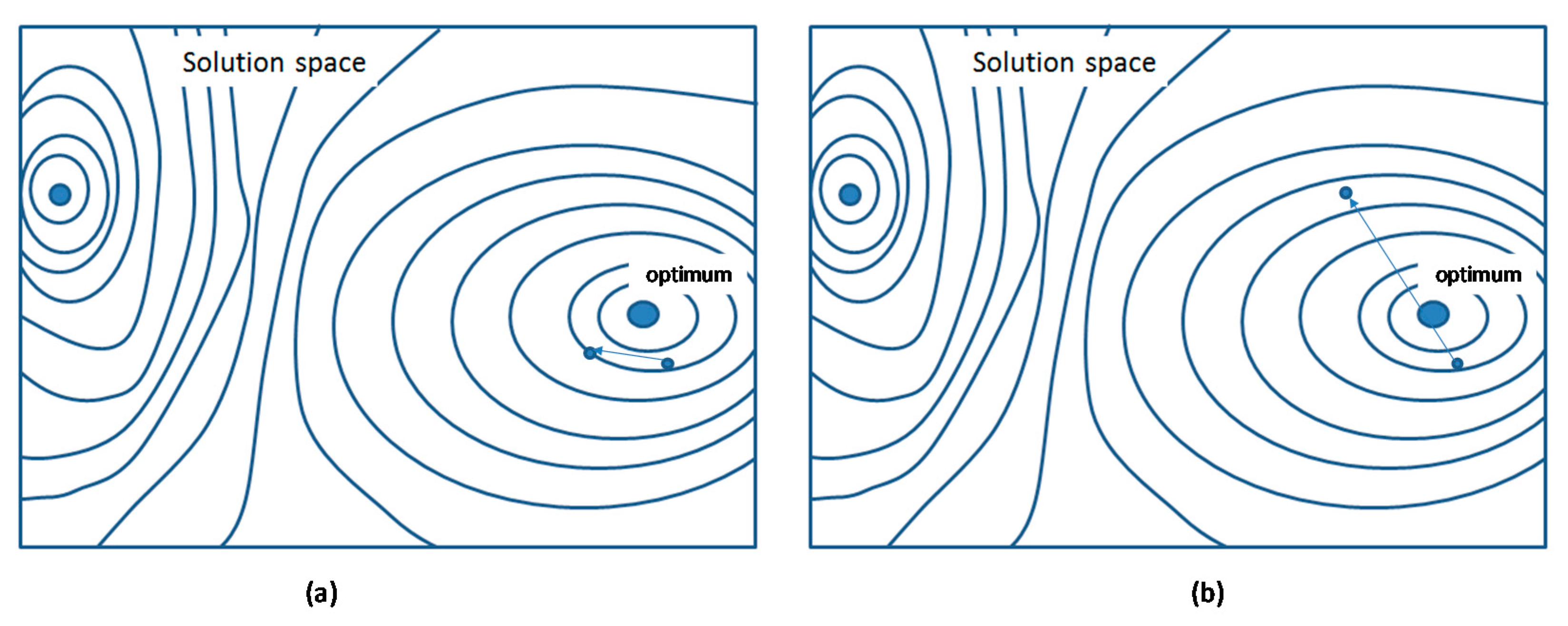
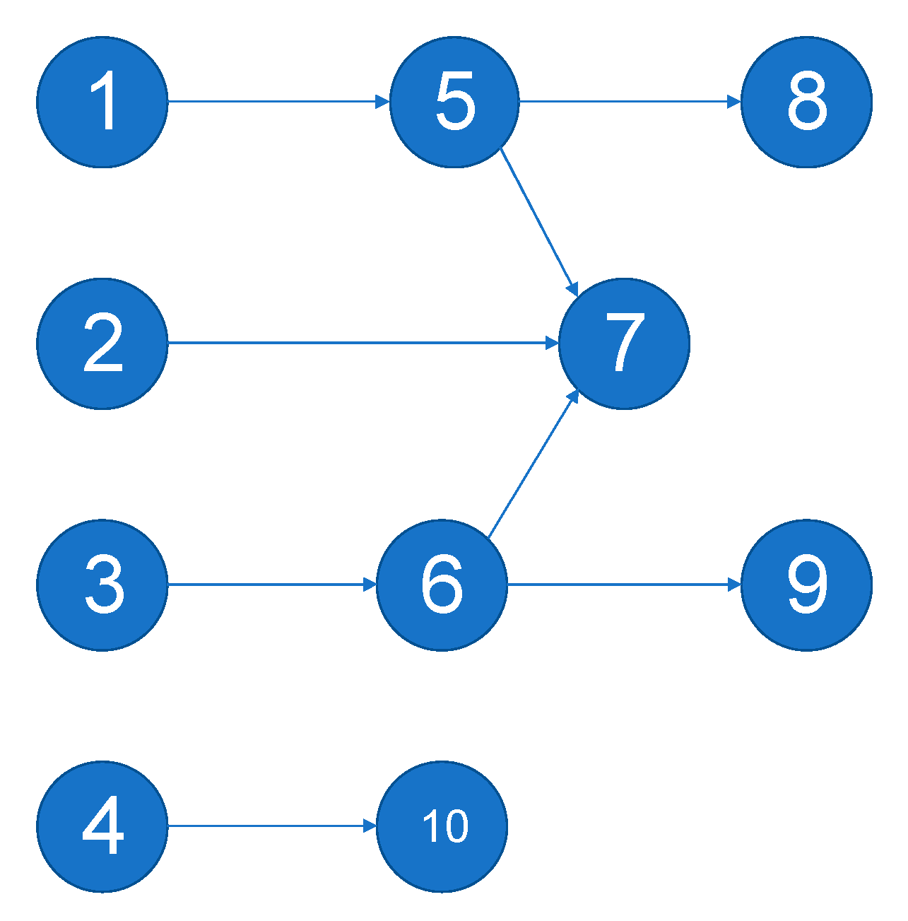
• Dependent projects: In the example depicted in Figure 4, Projects 5 and 6 have a common dependent in Project 7. This means that it will not be possible to gain the value of Project 7, even if Project 5 is expedited. There is a need to complete Projects 6 and 2 as well. Any small mutation expediting just one of these projects will leave the others untouched and fail to yield a major gain in value. Furthermore, any mutation that causes one of these projects to be postponed will yield a major reduction in the total value. A mutation involving all three projects may enable the expedition of the lucrative Project 7. The proposed similarity measure is (based on [65])

  $$\mathbb{S}{1}_{k,m}=\frac{{{\displaystyle \sum }}_{i=1}^N{d}_{k,i}{d}_{m,i}}{{{\displaystyle \sum }}_{i=1}^N{d}_{k,i}\left(1-d_{m,i}\right)+{{\displaystyle \sum }}_{i=1}^N{d}_{m,i}\left(1-d_{k,i}\right)+{{\displaystyle \sum }}_{i=1}^N{d}_{k,i}{d}_{m,i}}$$

  (11)

  where the latter is simply the number of projects that depend on both project $k$ and $m$ divided by the number of projects that depend on either of the two. For example, $\mathbb{S}{1}_{5,6}=\frac{1}{1+1+1}=\frac{1}{3}$, since only Project 7 depends on both projects, and there are 3 projects that depend on either 5 or 6.
• Mutual dependencies: When two projects depend on the same (or nearly the same) projects, expediting both together causes only a little more impact on the entire schedule than expediting only one (i.e., “two for almost the same price”). Therefore, the second similarity is calculated as follows:

  $$\mathbb{S}{2}_{k,m}=\frac{{{\displaystyle \sum }}_{i=1}^N{d}_{i,k}{d}_{i,m}}{{{\displaystyle \sum }}_{i=1}^N{d}_{i,m}\left(1-d_{i,m}\right)+{{\displaystyle \sum }}_{i=1}^N{d}_{i,m}\left(1-d_{i,k}\right)+{{\displaystyle \sum }}_{i=1}^N{d}_{i,k}{d}_{i,m}}$$

  (12)
• Resource requirements: Obviously, all projects compete for the same resource pool. Therefore, the third similarity is based on the measure of the level of common resources required by both projects. Two projects that require totally different resources do not compete at all. Projects that compete for the same resource, in which the resource itself is in abundance, will result in a minimal competition. If, however, both have high requirements for a low-level resource, then they are in head-to-head competition. Therefore, the third similarity can be calculated as the ratio between the required combined resources and the availability of these resources:

  $$s{3}_{k,m}={\displaystyle \sum }_{j=1}^R\frac{q_{j,k}+q_{j,m}}{{{\displaystyle \sum }}_{i=1}^H{r}_{j,i}}$$

  (13)
• This similarity measure differs from $\mathbb{S}1$ and $\mathbb{S}2$. First, it measures dissimilarity. Second, the value of $s3$ depends on the number of resources ($R$). The larger the value of $R$, the larger the value of $s3$. This poses a problem for the implementation of the CLONALG method. Therefore, the similarity measure ($\mathbb{S}{3}_{k,m}$) will be calculated as follows:

  $$\mathbb{S}{3}_{k,m}=\frac{1-s{3}_{k,m}}{\underset{\forall n\ne p}{\max }(1-s{3}_{n,p})}$$

  (14)

Thus, the similarity measure ($\mathbb{S}3$) is set to be a 0–1 number, where 1 indicates 2 non-competing projects, and the lower the value, the higher the competition for resources.

These three similarity measures are utilized to create a similarity coefficient that incorporates all these attributes. The similarity coefficient is, therefore, the following:

$$\mathbb{S}{ℂ}_{k,m}={\alpha }_1\mathbb{S}{1}_{k,m}+{\alpha }_2\mathbb{S}{2}_{k,m}+{\alpha }_3\mathbb{S}{3}_{k,m}$$

(15)

where ${\alpha }_1+{\alpha }_2+{\alpha }_3=1$ and ${\alpha }_1,{\alpha }_2,{\alpha }_3$ are non-negative.

The similarity coefficient is the base of the mutation generation algorithm:

• Randomly choose a project $k$;
• Create an empty set of projects $\mathsf{\Phi }$;
• For each project $m=1\dots N$ where $m\ne k$, do the following:

  3.1

  Generate a random number $u~U\left(0,1\right)$;

  3.2

  If $\mathbb{S}{ℂ}_{k,m}>u$, then add project $m$ to $\mathsf{\Phi }$.

• Randomly choose a location $l$ for project $k$;
• Move all members of the set $\mathsf{\Phi }$ to location $l$ (while maintaining the inner order of $\mathsf{\Phi }$).

6.4. Mixed Mutations

The basic concept of the oriented mutations is that the advance toward the optimum is not limited to random mutations but also benefits from knowledge and common sense (as expressed in the similarity coefficient matrix). In Figure 7a, there is an illustration of random mutations, where the new solutions are spread randomly. Figure 7b depicts an illustration of the oriented mutations, where the new solutions are concentrated in the vicinities of the optima.

The main risk of the oriented mutation is that the “orientation” will lower the diversification, or the ability to visit many different regions of the solution space [66]. Lower diversification will interfere with the random search and disturb the metaheuristic process that enables escape from the local optima. Though the oriented approach increases the search intensification, it is essential to find an optimal balance between intensification and diversification [67].

To overcome this risk, other approaches were examined for the mutation process. These approaches were basically to tune the level of similarity that is, in the mutation algorithm depicted in Section 6.2, Step 3 is replaced by the following:

3

For each project $m=1\dots N$ where $m\ne k$, do the following:

3.1

Generate a random number $u~U\left(0,1\right)$;

3.2

If $\alpha \mathbb{S}{ℂ}_{k,m}>u$, then add project $m$ to $\mathsf{\Phi }$.

where $\alpha$ is the tuning parameter. A high value of $\alpha$ means that the mutation process relies more on oriented mutations. A low value of $\alpha$ means it is less reliant on these. When $\alpha =0$, the mutation process is the same as depicted in Section 6.2.

7. Computational Results

7.1. Database

To examine the performance of the different approaches, a random data set of portfolios was generated. To encompass the wide variety of portfolios, the database was generated by randomly generating different cases varying in size, connectivity, and resources:

• Size: The number of projects varied between 20 and 120 projects (20, 40, 60, and 80 projects);
• Connectivity: The number of precedence connections can vary between zero (i.e., no project depends on any other one) and full connectivity (i.e., all projects can be presented as Project 1 precedes Project 2, which precedes Project 3, and so on). The problems were divided into three categories: high, low, and medium connectivity;
• Resources: For each type of resource, its scarcity can be measured by the ratio between the total demand (of all projects) and its annual availability. The resource scarcity has a strong connection to the planning horizon (the scarcer the resource, the more years are needed to complete the entire set of projects). As the number of years for the entire project was set to five, the scarcest resource was set to require seven times the annual resource level. The total number of resources varied between 1 and 3.

For each combination of size, connectivity, and resources, a set of five random portfolios was generated.

The data set was planned for 5 years (a project scheduled for year 6 is considered to be undesired and not performed).

7.2. Experiment Design

The purpose of the experiment was to assess the performance of the four approaches to CLONALG mutations (i.e., minor, major, oriented, and mixed mutations). As there was no database of optimal (or even best-known) solutions, the comparison was based on the following measures:

• Ratio to optimal solution: For smaller problems (i.e., sets of 20 projects), an optimal solution was found using B&B;
• Ratio to best-known solution: For each instance, the best value was found, and for each method, the ratio between its solution and the best solution was calculated.

To compare the various methods correctly, they were run for the exact same time. The runtime for each problem was set by running the minor mutation first until no improvement was achieved for 20 generations. The time was measured, and then all other methods were run for the same length of time, thus providing a comfortable benchmark.

The mixed method used a value of $\alpha =0.5$.

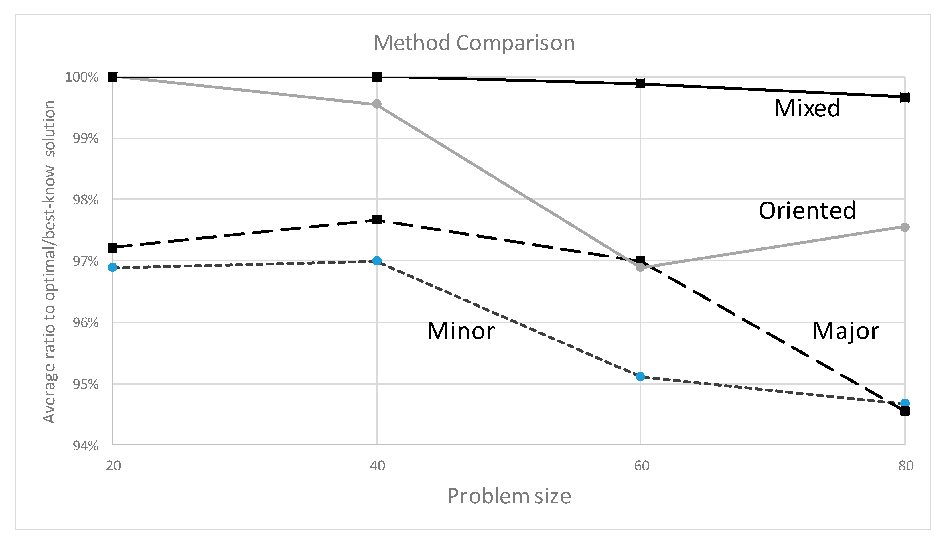
7.3. Initial Results

The results of the experiment for small problems are depicted in

Table 3. Initial results: ratio to optimal solutions.

Connectivity	Resources	Minor	Major	Oriented	Mixed
Low	1	1	1	1	1
	2	0.94	0.94	1	1
	3	0.93	0.96	1	1
Med	1	1	1	1	1
	2	0.96	1	1	1
	3	0.93	0.94	1	1
High	1	1	1	1	1
	2	0.96	0.96	1	1
	3	1	0.95	1	1

. For larger problems, the results are depicted in

Table 4. Initial results: ratio to optimal best known.

Problem Size	Connectivity	Resources	Minor	Major	Oriented	Mixed
40	Low	1	1	1	1	1
		2	0.94	0.96	1	1
		3	0.93	0.93	0.96	1
	Med	1	1	1	1	1
		2	0.96	1	1	1
		3	0.94	0.94	1	1
	High	1	1	1	1	1
		2	0.96	0.96	1	1
		3	1	1	1	1
60	Low	1	0.95	1	1	1
		2	0.99	0.98	0.96	1
		3	0.91	0.95	0.96	1
	Med	1	0.97	1	1	1
		2	0.91	1	0.94	0.99
		3	0.99	0.97	0.95	1
	High	1	0.96	0.96	0.93	1
		2	0.95	0.97	1	1
		3	0.93	0.9	0.98	1
80	Low	1	0.91	0.92	1	1
		2	1	0.93	0.97	1
		3	0.99	0.94	0.96	0.99
	Med	1	0.9	0.96	0.97	1
		2	0.93	0.96	1	1
		3	0.94	0.96	0.96	1
	High	1	0.97	0.91	0.99	1
		2	0.91	0.99	0.97	1
		3	0.97	0.94	0.96	0.98

.

As can be seen from Table 3 and Table 4, the mixed method outperformed all other methods (also relying only on minor mutations proven to be underperforming). A comparison between the methods is described in Figure 8.

The graph of Figure 8 reveals that the “oriented” (i.e., Lamarckian) mutations indeed improved the performance of the metaheuristic search. However, mixing them with “classic” mutations provided better solutions. The question that arises is the composition of this mix. The experiment was based on the arbitrary setting of $\alpha =0.5$ (i.e., halfway between oriented mutations and totally non-oriented ones). As the advantage of oriented mutations was established, it is interesting to further explore and find the optimal ratio of this “mix”.

To test this point, a second experiment was performed. The same sets of 80 problems were used again for different values of $\alpha$. The results are depicted in Figure 9. From the results, it is evident that there was almost no significance to the value of α as long as there was a presence of oriented mutations and as long as the oriented mutations monopolized the process.

8. Summary and Conclusions

This paper aimed to tackle the problem of project selection subject to resource constraints and technical precedence. To test this novel problem, the research developed a benchmark database of portfolios varying in size, precedence complexity, and resources. As far as we can ascertain, this is a one-of-a-kind database, and one of the outcomes of this research is to set benchmark results. This paper provides an exact formulation and an example for the new problem.

To solve the problem, a practical search approach for reaching a solution was developed. This enhancement approach would be applicable for most metaheuristic search techniques by using clustering methods that portray the attractive search zones and act as “intensificators”. The proposed search was able to generate feasible, meaningful, and highly satisfactory solutions to the planning of long-horizon problems.

The proposed algorithm has both theoretical and practical implications. The practical one is its ability to upgrade the PPS problem decision making and base it on solid exact foundations. The decision-making process should be based less on “gut feelings” and more on exact and well-presented data. Furthermore, the process may enable the decision makers to be aware of the impact of various constraints and lead to improved decisions (e.g., the economic benefit of recruiting more of a specific type of engineers). The theoretical implications, on the other hand, can be derived from the metaheuristic approach; the suggested oriented search need not be limited to PPS and can be implemented in various scheduling (and perhaps other) problems.

An obvious weakness of the article is its limitation to a specific problem, where the data is deterministic and the objective function is limited to a single one (maximum gain value). In reality, the data are often fuzzy or stochastic, and the proposed model does not take this into account. It is worth mentioning that there is nothing fundamental that prevents the proposed meta-heuristic search techniques from tackling fuzzy objective functions, and this may be a suitable direction for further research.

Another direction for future research could use the presented insights to develop better algorithms that will smartly manipulate the mutation type in the different phases of the search and develop a technique or a method for optimizing the various factors of the search to better its performance.

References

1. Tavana, M.; Keramatpour, M.; Santos-Arteaga, F.J.; Ghorbaniane, E. A fuzzy hybrid project portfolio selection method using Data Envelopment Analysis, TOPSIS and Integer Programming. Expert Syst. Appl. 2015, 42, 8432–8444. [Google Scholar] [CrossRef]
2. Gutiérrez, E.; Magnusson, M. Dealing with legitimacy: A key challenge for Project Portfolio Management decision makers. Int. J. Proj. Manag. 2014, 32, 30–39. [Google Scholar] [CrossRef]
3. Jonas, D. Empowering project portfolio managers: How management involvement impacts project portfolio management performance. Int. J. Proj. Manag. 2010, 28, 818–831. [Google Scholar] [CrossRef]
4. Killen, C.; Hunt, R. Dynamic capability through project portfolio management in service and manufacturing industries. Int. J. Manag. Proj. Bus. 2010, 3, 157–169. [Google Scholar] [CrossRef] [Green Version]
5. Meskendahl, S. The influence of business strategy on project portfolio management and its success—a conceptual framework. Int. J. Proj. Manag. 2010, 28, 807–817. [Google Scholar] [CrossRef]
6. Lechler, T.G.; Thomas, J.L. Examining new product development project termination decision quality at the portfolio level: Consequences of dysfunctional executive advocacy. Int. J. Proj. Manag. 2015, 33, 1452–1463. [Google Scholar] [CrossRef]
7. Martinsuo, M. Project portfolio management in practice and in context. Int. J. Proj. Manag. 2013, 31, 794–803. [Google Scholar] [CrossRef]
8. Pendharkar, P.C. A decision-making framework for justifying a portfolio of IT projects. Int. J. Proj. Manag. 2014, 32, 625–639. [Google Scholar] [CrossRef]
9. Dutra, C.C.; Ribeiro, J.L.D.; de Carvalho, M.M. An economic–probabilistic model for project selection and prioritization. Int. J. Proj. Manag. 2014, 32, 1042–1055. [Google Scholar] [CrossRef]
10. Meade, L.M.; Presley, A. R&D project selection using the analytic network process. IEEE Trans. Eng. Manag. 2002, 49, 59–66. [Google Scholar]
11. Jafarzadeh, M.; Tareghian, H.R.; Rahbarnia, F.; Ghanbari, R. Optima lselection of project portfolios using reinvestment strategy within a flexible time horizon. Eur. J. Oper. Res. 2015, 243, 658–664. [Google Scholar] [CrossRef]
12. Frey, T.; Buxmann, P. IT Project Portfolio Management—A Structured Literature Review. In Proceedings of the 20th European Conference on Information Systems, Barcelona, Spain, 10–13 June 2012. [Google Scholar]
13. Weissenberger-Eibl, M.A.; Teufel, B. Organizational politics in new product development project selection. Eur. J. Innov. Manag. 2011, 14, 51–73. [Google Scholar] [CrossRef]
14. Padhy, R. Six Sigma project selections: A critical review. Int. J. Lean Six Sigma 2017, 8, 244–258. [Google Scholar] [CrossRef]
15. Condé, G.C.P.; Mauro, L.M. Six sigma project generation and selection: Literature review and feature based method proposition. Prod. Plan. Control. 2020, 31, 1303–1312. [Google Scholar] [CrossRef]
16. Danesh, D.; Ryan, M.J.; Abbasi, A. Multi-criteria decision-making methods for project portfolio management: A literature review. Int. J. Manag. Decis. Mak. 2018, 17, 75–94. [Google Scholar] [CrossRef]
17. Mohagheghi, V.; Mousavi, S.M.; Antuchevičienė, J.; Mojtahedi, M. Project portfolio selection problems: A review of models, uncertainty approaches, solution techniques, and case studies. Technol. Econ. Dev. Econ. 2019, 25, 1380–1412. [Google Scholar] [CrossRef]
18. Hall, N.G.; Long, D.Z.; Qi, J.; Sim, M. Managing underperformance risk in project portfolio selection. Oper. Res. 2015, 63, 660–675. [Google Scholar] [CrossRef] [Green Version]
19. Tofighian, A.A.; Naderi, B. Modeling and solving the project selection and scheduling. Comput. Ind. Eng. 2015, 83, 30–38. [Google Scholar] [CrossRef]
20. Gutjahr, W.J.; Reiter, P. Bi-objective project portfolio selection and staff assignment under uncertainty. Optimization 2010, 59, 417–445. [Google Scholar] [CrossRef]
21. Ghapanchi, A.H.; Tavana, M.; Khakbaz, M.H.; Low, G. A methodology for selecting portfolios of projects with interactions and under uncertainty. Int. J. Proj. Manag. 2012, 30, 791–803. [Google Scholar] [CrossRef]
22. Mutavdzic, M.; Maybee, B. An extension of portfolio theory in selecting projects to construct a preferred portfolio of petroleum assets. J. Pet. Sci. Eng. 2015, 133, 518–528. [Google Scholar] [CrossRef]
23. Arratia, N.M.; Lόpez, F.; Schaeffer, S.E.; Cruz-Reyes, L. Static R&D project portfolio selection in public organizations. Decis. Support Syst. 2016, 84, 53–63. [Google Scholar]
24. Kalashnikov, V.; Benita, F.; López-Ramos, F.; Hernández-Luna, A. Bi-objective project portfolio selection in Lean Six Sigma. Int. J. Prod. Econ. 2017, 186, 81–88. [Google Scholar] [CrossRef]
25. Guo, Y.; Wang, L.; Li, S.; Chen, Z.; Cheng, Y. Balancing strategic contributions and financial returns: A project portfolio selection model under uncertainty. Soft Comput. 2018, 22, 5547–5559. [Google Scholar] [CrossRef]
26. Carazo, A.F.; Gómez, T.; Molina, J.; Hernández-Díaz, A.G.; Guerrero, F.M.; Caballero, R. Solving a comprehensive model for multiobjective project portfolio selection. Comput. Oper. Res. 2010, 37, 630–639. [Google Scholar] [CrossRef]
27. Kremmel, T.; Kubalík, J.; Biffl, S. Software project portfolio optimization with advanced multiobjective evolutionary algorithms. Appl. Soft Comput. 2011, 11, 1416–1426. [Google Scholar] [CrossRef]
28. Liesiö, J.; Punkka, A. Baseline value specification and sensitivity analysis in multiattribute project portfolio selection. Eur. J. Oper. Res. 2014, 237, 946–956. [Google Scholar] [CrossRef]
29. Hassanzadeh, F.; Nemati, H.; Sun, M. Robust optimization for interactive multiobjective programming with imprecise information applied to R&D project portfolio selection. Eur. J. Oper. Res. 2014, 238, 41–53. [Google Scholar]
30. Shou, Y.; Xiang, W.; Li, Y.; Yao, W. A multiagent evolutionary algorithm for the resource-constrained project portfolio selection and scheduling problem. Math. Probl. Eng. 2014, 2014, 302684. [Google Scholar] [CrossRef] [Green Version]
31. Dehouche, N. Non-profit project portfolio evaluation and selection: A multi-criteria approach. Int. J. Appl. Manag. Sci. 2015, 7, 338–363. [Google Scholar] [CrossRef]
32. Fliedner, T.; Liesiö, J. Adjustable robustness for multi-attribute project portfolio selection. Eur. J. Oper. Res. 2016, 252, 931–946. [Google Scholar] [CrossRef]
33. Perez, F.; Gomez, T. Multiobjective project portfolio selection with fuzzy constraints. Ann. Oper. Res. 2016, 245, 7–29. [Google Scholar] [CrossRef]
34. Danesh, D.; Ryan, M.J.; Abbasi, A. A systematic comparison of multi-criteria decision making methods for the improvement of project portfolio management in complex organisations. Int. J. Manag. Decis. Mak. 2017, 16, 280–320. [Google Scholar]
35. Ehsani, E.; Kazemi, N.; Olugu, E.U.; Grosse, E.H.; Schwindl, K. Applying fuzzy multi-objective linear programming to a project management decision with nonlinear fuzzy membership functions. Neural Comput. Appl. 2017, 28, 2193–2206. [Google Scholar] [CrossRef]
36. El-Kholany, M.M.; Abdelsalam, H.M. Multi-objective binary cuckoo search for constrained project portfolio selection under uncertainty. Eur. J. Ind. Eng. 2017, 11, 818–853. [Google Scholar] [CrossRef]
37. Liu, F.; Chen, Y.W.; Yang, J.B.; Xu, D.L.; Liu, W. Solving multiple-criteria R&D project selection problems with a data-driven evidential reasoning rule. Int. J. Proj. Manag. 2019, 37, 87–97. [Google Scholar]
38. Pérez, F.; Gómez, T.; Caballero, R.; Liern, V. Project portfolio selection and planning with fuzzy constraints. Technol. Forecast. Soc. Chang. 2018, 131, 117–129. [Google Scholar] [CrossRef]
39. Liu, Y.; Liu, Y.-K. Distributionally robust fuzzy project portfolio optimization problem with interactive returns. Appl. Soft Comput. 2017, 56, 655–668. [Google Scholar] [CrossRef]
40. Takami, M.A.; Sheikh, R.; Sana, S.S. A Hesitant Fuzzy Set Theory Based Approach for Project Portfolio Selection with Interactions under Uncertainty. J. Inf. Sci. Eng. 2018, 34, 65–79. [Google Scholar]
41. Naderi, B. The project portfolio selection and scheduling problem: Mathematical model and algorithms. J. Optim. Ind. Eng. 2013, 6, 65–72. [Google Scholar]
42. Wang, B.; Song, Y. Reinvestment Strategy-Based Project Portfolio Selection and Scheduling with Time-Dependent Budget Limit Considering Time Value of Capital. In Proceedings of the 2015 International Conference on Electrical and Information Technologies for Rail Transportation, Zhuzhou, China, 17–19 October 2015; Springer: Berlin/Heidelberg, Germany, 2016; pp. 373–381. [Google Scholar]
43. Martínez-Vega, D.A.; Cruz-Reyes, L.; Rangel-Valdez, N.; Santillán, C.G.; Sánchez-Solís, P.; Villafuerte, M.P. Project portfolio selection with scheduling: An evolutionary approach. Int. J. Comb. Optim. Probl. Inform. 2019, 10, 25–31. [Google Scholar]
44. Killen, C.P.; Jugdev, K.; Drouin, N.; Petit, Y. Advancing project and portfolio management research: Applying strategic management theories. Int. J. Proj. Manag. 2012, 30, 525–538. [Google Scholar] [CrossRef]
45. Jeng, D.J.-F.; Huang, K.-H. Strategic project portfolio selection for national research institutes. J. Bus. Res. 2015, 68, 2305–2311. [Google Scholar] [CrossRef]
46. Kopmann, J.; Kock, A.; Killen, C.P.; Gemünden, H.G. The role of project portfolio management in fostering both deliberate and emergent strategy. Int. J. Proj. Manag. 2017, 35, 557–570. [Google Scholar] [CrossRef] [Green Version]
47. Kaiser, M.G.; el Arbi, F.; Ahlemann, F. Successful project portfolio management beyond project selection techniques: Understanding the role of structural alignment. Int. J. Proj. Manag. 2015, 33, 126–139. [Google Scholar] [CrossRef]
48. Hoof, V.; Broeckx, F. Specification of Queuing Models: An Alternative Notation. Int. J. Model. Simul. 1982, 2, 67–70. [Google Scholar] [CrossRef]
49. Pajares, J.; López, A. New Methodological Approaches to Project Portfolio Management: The Role of Interactions within Projects and Portfolios. Procedia—Soc. Behav. Sci. 2014, 119, 645–652. [Google Scholar] [CrossRef] [Green Version]
50. Shariatmadari, M.; Nahavandi, N.; Zegordi, S.H.; Mohammad, H.S. Integrated resource management for simultaneous project selection and scheduling. Comput. Ind. Eng. 2017, 109, 39–47. [Google Scholar] [CrossRef]
51. Li, X.; Fang, S.-C.; Tian, Y.; Guo, X. Expanded model of the project portfolio selection problem with divisibility, time profile factors and cardinality constraints. J. Oper. Res. Soc. 2015, 66, 1132–1139. [Google Scholar] [CrossRef]
52. Rafiee, M.; Kianfar, F.; Farhadkhani, M. A multistage stochastic programming approach in project selection and scheduling. Int. J. Adv. Manuf. Technol. 2014, 70, 2125–2137. [Google Scholar] [CrossRef]
53. Sefair, J.A.; Méndez, C.Y.; Babat, O.; Medaglia, A.L.; Zuluaga, L.F. Linear solution schemes for Mean-SemiVariance Project portfolio selection problems: An application in the oil and gas industry. Omega 2018, 68, 39–48. [Google Scholar] [CrossRef]
54. Samphaiboon, N.; Yamada, T. Heuristic and exact algorithms for the precedence-constrained knapsack problem. J. Optim. Theory Appl. 2000, 105, 659–676. [Google Scholar] [CrossRef]
55. de Castro, L.; von Zuben, F.J. The Clonal Selection Algorithm with Engineering Applications. In Proceedings of the Workshop on Artificial Immune Systems and Their Applications, Las Vegas, NV, USA, 8–12 July 2000. [Google Scholar]
56. Swain, R.K.; Barisal, A.K.; Hota, P.K.; Chakrabarti, R. Short-term hydrothermal scheduling using clonal selection algorithm. Int. J. Electr. Power Energy Syst. 2011, 33, 647–656. [Google Scholar] [CrossRef]
57. Attwater, J.; Holliger, P. The cooperative gene. Nature 2012, 491, 48–49. [Google Scholar] [CrossRef] [PubMed]
58. Bohl, K.; Hummert, S.; Werner, S.; Basanta, D.; Deutsch, A.; Schuster, S.; Theißen, G.; Schroeter, A. Evolutionary game theory: Molecules as players. Mol. BioSyst. 2014, 10, 3066–3074. [Google Scholar] [CrossRef] [Green Version]
59. Furubayashi, T.; Ueda, K.; Bansho, Y.; Motooka, D.; Nakamura, S.; Mizuuchi, R.; Ichihashi, N. Emergence and diversification of a host-parasite RNA ecosystem through Darwinian evolution. Elife 2020, 9, e56038. [Google Scholar] [CrossRef]
60. Seifoddini, H.; Wolfe, P.M. Application of the similarity coefficient method in group technology. IIE Trans. 1986, 18, 271–277. [Google Scholar] [CrossRef]
61. Selim, H.M.; Askin, R.G.; Vakharia, A.J. Cell formation in group technology: Review, evaluation and directions for future research. Comput. Ind. Eng. 1998, 34, 3–20. [Google Scholar] [CrossRef]
62. Lu, P.; Zhang, Z. Critical nodes identification in complex networks via similarity coefficient. Mod. Phys. Lett. B 2022, 36, 2150620. [Google Scholar] [CrossRef]
63. Wu, L.; Shen, Y.; Niu, B.; Li, L.; Yang, C.; Feng, Y. Similarity coefficient-based cell formation method considering operation sequence with repeated operations. Eng. Optim. 2021, 22, 1–15. [Google Scholar] [CrossRef]
64. Yang, Z.; Qiao, T.; Ren, J.; Yuen, P.; Zhao, H.; Sun, G.; Marshall, S.; Benediktsson, J.A. Joint bilateral filtering and spectral similarity-based sparse representation: A generic framework for effective feature extraction and data classification in hyperspectral imaging. Pattern Recognit. 2018, 77, 316–328. [Google Scholar]
65. Erlich, Z.; Gelbard, R.; Spiegler, I. Data Mining by Means of Binary Representation: A Model for Similarity and Clustering. Inf. Syst. Front. 2002, 4, 187–197. [Google Scholar] [CrossRef]
66. Lozano, M.; García-Martínez, C. Hybrid metaheuristics with evolutionary algorithms specializing in intensification and diversification: Overview and progress report. Comput. Oper. Res. 2010, 37, 481–497. [Google Scholar] [CrossRef]
67. Scheibenpflug, A.; Wagner, S. An Analysis of the Intensification and Diversification Behavior of Different Operators for Genetic Algorithms. In Proceedings of the 14th International Conference on Computer Aided Systems Theory, Las Palmas, Spain, 10–15 February 2013. [Google Scholar]
Figure 1. Project portfolio selection classification scheme.
Mathematics 10 01601 g001
Figure 2. A simple mutation.
Mathematics 10 01601 g002
Figure 3. (a) A small mutation. (b) A large mutation.
Mathematics 10 01601 g003
Figure 4. Projects’ dependencies.
Mathematics 10 01601 g004
Figure 5. Comparison between the advantages of (a) large and (b) small mutations.
Mathematics 10 01601 g005
Figure 6. Switch mutation.
Mathematics 10 01601 g006
Figure 7. (a) Random mutations vs. (b) Oriented mutations.
Mathematics 10 01601 g007
Figure 8. Comparison.
Mathematics 10 01601 g008
Figure 9. Effect of α.
Mathematics 10 01601 g009