STAGCN: Spatial–Temporal Attention Graph Convolution Network for Traffic Forecasting

Abstract

Traffic forecasting plays an important role in intelligent transportation systems. However, the prediction task is highly challenging due to the mixture of global and local spatiotemporal dependencies involved in traffic data. Existing graph neural networks (GNNs) typically capture spatial dependencies with the predefined or learnable static graph structure, ignoring the hidden dynamic patterns in traffic networks. Meanwhile, most recurrent neural networks (RNNs) or convolutional neural networks (CNNs) cannot effectively capture temporal correlations, especially for long-term temporal dependencies. In this paper, we propose a spatial–temporal attention graph convolution network (STAGCN), which acquires a static graph and a dynamic graph from data without any prior knowledge. The static graph aims to model global space adaptability, and the dynamic graph is designed to capture local dynamics in the traffic network. A gated temporal attention module is further introduced for long-term temporal dependencies, where a causal-trend attention mechanism is proposed to increase the awareness of causality and local trends in time series. Extensive experiments on four real-world traffic flow datasets demonstrate that STAGCN achieves an outstanding prediction accuracy improvement over existing solutions.

1. Introduction

Traffic forecasting aims to predict future traffic conditions (e.g., traffic flow, interval speed) based on historical traffic information that is as long as the prediction interval. In general, traffic prediction tasks can be divided into two categories according to the length of the prediction interval, namely short-term (5~30 min) and long-term (30~60 min) prediction tasks [1]. Traffic forecasting also plays an important role in Intelligent Transportation Systems (ITS), and it remains challenging due to its complex and changing spatial–temporal dependencies in real-world road networks [2]. Traditional forecasting methods, such as the autoregressive integrated moving average (ARIMA) model [3] and Kalman filter [4], have a solid theoretical foundation, but they must rely on the stationarity assumption. Furthermore, these methods are mainly applied to univariate time series, which restricts their applications in real-world scenarios. With the development of data availability and information computation, deep learning-based prediction work achieves remarkable performance. Deep neural networks for spatiotemporal sequence modeling are mainly divided into three categories: recurrent neural networks (RNNs), convolutional neural networks (CNNs), and graph convolutional networks (GCNs) [5]. RNN-based approaches employ hidden recurrent units to retain historical information, but they may suffer from vanishing gradient issues when modeling long-term temporal dependencies (i.e., temporal correlations between distant time steps in long sequences). CNN-based approaches propagate spatiotemporal information under the assumption that traffic data are generated from grid-distributed sensors, and they fail to explicitly capture spatial correlations in non-Euclidean data. GCN-based approaches receive widespread attention due to their high adaptability in dealing with non-Euclidean data. At present, most GCNs rely on the predefined static graph structure with prior knowledge. A fine-grained graph structure will bring great improvements for prediction performance, and how to obtain the optimal graph structure becomes a primary challenge. In most cases, complex spatiotemporal data are not equipped with an explicit graph structure, because connections among arbitrary nodes (e.g., sensors of traffic network) should be generated in a data-oriented manner. Graph WaveNet [6] proposes a self-adaptive adjacency matrix to preserve hidden spatial correlations. Wu et al. [7] extract a sparse graph adjacency matrix adaptively based on data and updates the matrix during training. Yu et al. [8] introduce iterative learning for graph learning by leveraging graph regularization. While the mentioned graph-based methods have been successfully used in real-world applications, including but not limited to action recognition, point cloud segmentation, and time series forecasting, they will still face the following challenges:

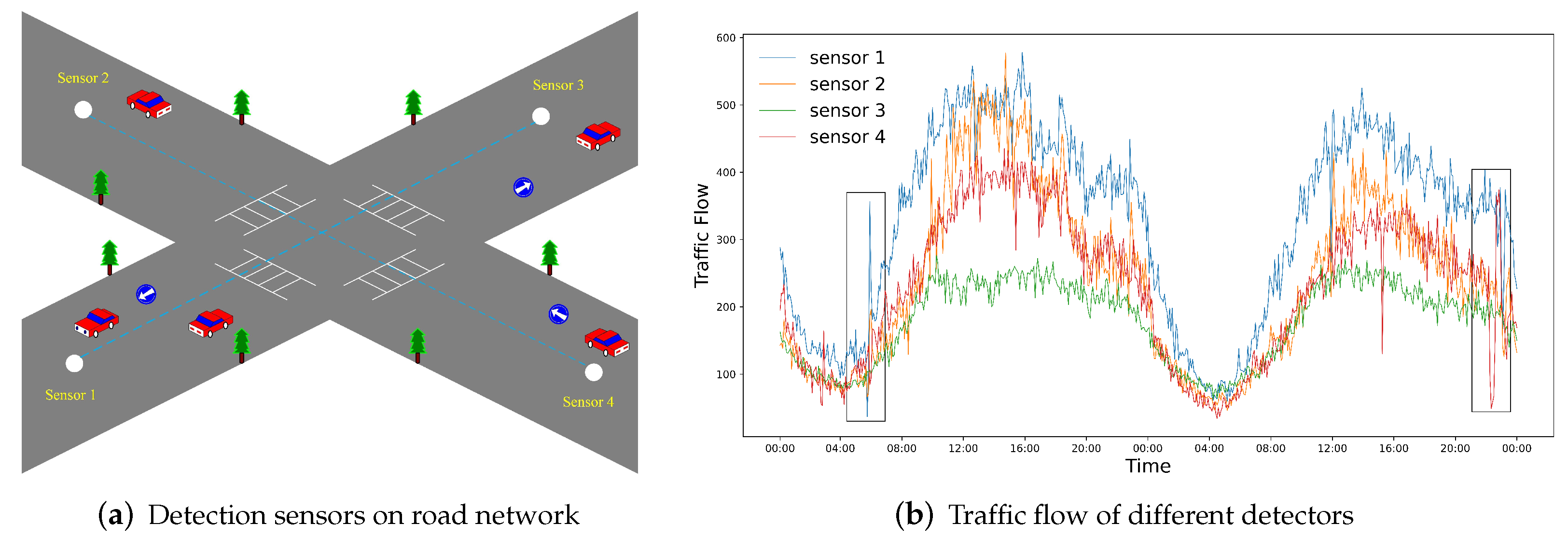
• Global adaptability and local dynamics. Most GCNs only focus on constructing an adaptive graph matrix to capture long-term or global space dependencies in traffic data, while overlooking the fact that the correlation between local nodes is changing significantly over time. As shown in Figure 1, sudden traffic accidents may lead to local changes in spatial correlation among nodes. The primary question is how to keep the balance between global adaptability and local dynamics in an end-to-end work.
• Long-term temporal correlations. Current graph-based methods are ineffective to model long-term temporal dependencies. Existing methods either integrate GCNs into RNNs or CNNs, in which small prediction errors at each time step may be magnified as the prediction interval grows. This type of error forward propagation makes long-term forecasting more challenging.

In this paper, we propose a novel approach to overcome the aforementioned challenges. Our framework consists of three components: graph learning layer, adaptive graph convolution layer, and gated temporal attention module. For challenge 1, we propose a graph learning layer in which two types of graph matrices can be learned from data, namely a static graph and dynamic graph. The static graph aims to explore global space adaptability in traffic graph networks, and graph regularization is further employed to control the quality of the static graph. The dynamic graph is designed to capture the locally changing information among nodes. For challenge 2, we propose a gated temporal attention module, which adopts multi-head self-attention to address long-term prediction issues. In contrast to RNNs and CNNs, the attention mechanism aggregates temporal features through a summation function with dynamically generated weights. This leads to an effective global receptive field and allows the model to focus on significant historical information, which can alleviate error forward propagation. To be more aware of causality and local trends in time series, we introduce a causal-trend attention mechanism instead of using traditional multi-head attention directly. In summary, our main contributions are as follows:

• We propose a novel graph learning layer to explore the interactions between global space adaptability and local dynamics in traffic networks without any guidance of prior knowledge. The static graph aims to model global adaptability, and the dynamic graph is designed to capture local spatial changes.
• We propose a gated temporal attention module to model long-term temporal dependencies. Furthermore, we design a causal-trend attention mechanism that enables our model to extract causality and local trends in time series.
• Extensive experiments are conducted on four public traffic datasets, and the experimental results show that our method consistently outperforms all baseline methods.

2. Related work

2.1. Traffic Forecasting

Traffic forecasting has been extensively studied in the past few decades. Earlier work is usually based on the traditional statistical methods, such as ARIMA and the Kalman filter. Although statistical methods are widely adopted for traffic forecasting due to their simplicity and interpretability, they have to rely on the stationary assumption and do not scale well for complex traffic data. Deep learning approaches can effectively capture the non-linearity of traffic data. Many of them initially employed RNNs [9] or TCNs [10] to model temporal dependency, ignoring the spatial correlations in traffic data. Later, researchers used CNNs [11] to extract spatial dependencies in Euclidean space, but this fails to effectively process non-Euclidean data and limits the prediction performance.

Recently, many studies have attempted to employ graph convolution methods to model spatial and temporal dependencies in non-Euclidean road networks. Most of them assume that a well-defined graph structure has already existed. Li et al. [12] integrate diffusion convolution into gated recurrent units (GRUs), where the predefined graph matrix is generated from road network distances. Now, many researchers are devoted to finding optimal graph structures in a data-driven way. Wang et al. [13] propose a new adaptive feature graph to learn correlations between topological structures and node features. Song et al. [14] propose a spatiotemporal graph to simultaneously capture the localized spatiotemporal dependencies, which requires prior graph knowledge and additional graph construction operation. The above graph-based methods mainly concentrate on adaptive graph construction or heavily rely on the predefined graph structure, ignoring dynamic correlations in traffic data.

2.2. Graph Convolutional Network

Graph convolutional networks (GCNs) have achieved extraordinary performance on several types of graph-based tasks, such as node classification [15], link prediction [16], and clustering [17]. From the perspective of convolution operators, GCNs have two mainstreams, namely spectral approaches and spatial approaches. Spectral approaches smooth graph signals in the spectral domain through Fourier transform. Spatial approaches define convolution operations directly on the graph based on the topology structure. Velickovic et al. [18] assign different weights to neighbor nodes via an attention mechanism. Li et al. [19] incorporate residual connections to increase the depth of GCNs and alleviates oversmoothing and vanishing gradient issues. In these methods, the graph adjacency matrix is regarded as prior knowledge and is static throughout the training phase. Wang et al. [20] employ distance metrics to adaptively learn a similarity graph weight matrix for label learning. The generated matrix relies on dynamic node representation and may hamper model performance on graphs where the node set keeps changing.

2.3. Attention Mechanism

The attention mechanism has been widely used in diverse application domains due to its high efficiency and flexibility in modeling dependencies. The core idea of the attention mechanism is to adaptively focus on significant parts when processing massive amounts of information. Fukui et al. [21] extend the attention mechanism to a response-based visual explanation model and achieves remarkable performance. Yan et al. [22] employ attention mechanisms to adaptively encode local and global point cloud context information. Zheng et al. [23] propose a spatiotemporal attention mechanism to explore dynamic spatial and non-linear temporal correlations. In this paper, we adopt an attention mechanism for long-term temporal dependency modeling.

3. Methodology

3.1. Preliminaries

Traffic Networks: The traffic prediction task can be expressed as a typical spatiotemporal series forecasting problem. We define the topological road network as a directed graph $G(V,A)$. Here, V is the set of $N=\left|V\right|$ vertices representing detectors installed on the road. The graph structure can be represented as a weighted adjacency matrix $A\in R^{N\times N}$, where $A_{i,j}>0$ indicates the correlation between vertices $v_i$ and $v_j$. In general, the values on the diagonal of the initialized adjacency matrix A are equal to 1, which could avoid ignoring the feature of the node itself. The traffic signals observed at time step t on traffic network G can be defined as $x^t\in R^{N\times C}$, where C denotes the feature dimension of vertices (e.g., traffic flow, traffic speed).

Problem Statement: Given the historical observed P time steps traffic signals, denoted as $X=\{x^{t_1},x^{t_2},\dots ,x^{t_p}\}\in R^{P\times N\times C}$, our goal is to predict next H time step traffic signals $Y=\{x^{t_{p+1}},x^{t_{p+2}},\dots ,x^{t_{p+h}}\}\in R^{H\times N\times C}$.

Scaled Dot-Product Attention: The attention function aims to map a query and a set of key–value pairs to an output, where the query and key–value pairs are all vectors. The output is a weighted sum of values, where the weight assigned to each value is determined jointly by a query and the corresponding key. The dot-product attention is a widely adopted attention function, which enjoys remarkable properties such as time and space efficiency. Finally, the output is as follows:

$$\mathrm{Attention}(\mathbf{Q},\mathbf{K},\mathbf{V})=SoftMax\left(\frac{\mathbf{Q}·{\mathbf{K}}^T}{\sqrt{d_k}}\right)\mathbf{V}.$$

(1)

where $\mathbf{Q}$, $\mathbf{K}$, $\mathbf{V}$, and $d_k$ represent the query, keys, values, and dimensions, respectively.

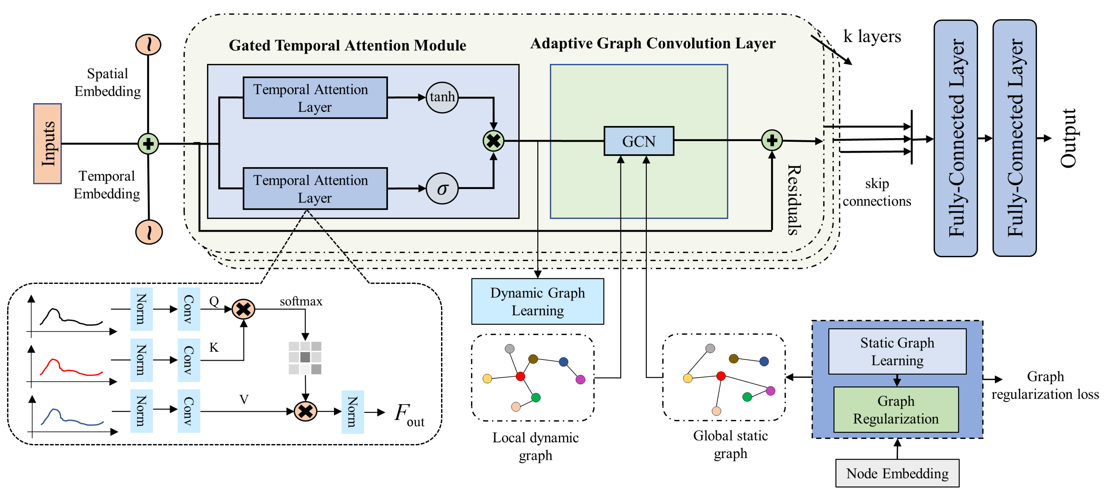
3.2. Framework of STAGCN

Figure 2 illustrates the architecture of our proposed STAGCN model, which consists of a static–dynamic graph learning layer, gated temporal attention module (Gated TAM), and adaptive graph convolution layer (GCN). To explore the complex correlations between global and local spatiotemporal dependencies, two types of graphs are learned from data, i.e., static graph and dynamic graph. Gated TAM consists of two parallel temporal attention layers, where causal-trend attention is proposed for long-term temporal dependencies. In GCN, we employ two separate modules to aggregate spatial information based on the static and dynamic graph. Every layer adopts residual connections and is skipped to the output module. In more detail, the core components of our model are illustrated in the following.

3.3. Spatial Static–Dynamic Graph Learning Layer

3.3.1. Static Graph Learning

The spatial static graph learning layer aims to learn a static adaptive adjacency matrix, which can capture the global spatial correlations among traffic data without the predefined graph structure. We employ node embedding to construct the static adjacency matrix [7,24], denoted as follows:

$$M_1=tanh(E_1·{\theta }_1),$$

(2)

$$M_2=tanh(E_2·{\theta }_2),$$

(3)

$$A_s=SoftMax\left(ReLU(M_1·M_2^T)\right),$$

(4)

where $E_1$, $E_2$ represent randomly initialized node embedding, whose parameters can be learned during training, and ${\theta }_1$, ${\theta }_2$ are model parameters. We employ $ReLU$ activation to eliminate weak connections between nodes. $SoftMax$ activation is adopted to normalize the learned adjacency matrix.

A well-defined graph structure can bring significant benefits to the prediction task, so it is essential to control the sparsity and smoothness of the learned graph structure. Therefore, we add a graph regularization loss function following previous work [8] to improve the quality of the graph structure. For the learned global adjacency matrix A and the given node feature matrix $X_F=(x_1,x_2,\dots ,x_N)\in R^{N\times D}$, the graph regularization loss is as follows:

$$L_G=\alpha \frac{1}{N^2}\sum _{i,j}^N{A}_{i,j}\parallel x_i-x_j{\parallel }^2+\beta {\parallel A\parallel }_F^2,$$

(5)

where $\alpha$, $\beta$ are model hyperparameters and ${\parallel ·\parallel }_F^2$ denotes the Frobenius norm of the matrix. A widely recognized assumption is that graph signals change smoothly through adjacent nodes, so minimizing the first term will force adjacent nodes to have similar features. However, only restricting the smoothness of the graph will lead to $A=0$, so we add the Frobenius norm of the matrix to control the sparsity of the graph. Instead of applying regularization to all inputs or node embedding at once, we apply it to the node output features in the gradient update section.

3.3.2. Dynamic Graph Learning

For spatiotemporal traffic data, the dependencies among nodes are very likely to dynamically change over time, e.g., traffic congestion upstream will affect the traffic flow downstream. Therefore, only applying the static graph structure may fail to grasp such local dynamic correlation. To this end, we introduce a dynamic graph that can adaptively alter the relationship among nodes at all time steps.

The key idea of our method is to adopt a self-attention mechanism to calculate the spatial correlations among nodes. To be concrete, given the dynamic node feature set $X_t\in R^{N\times d_{model}}$, the dynamic spatial adjacency matrix can be denoted as:

$$A_d=SoftMax\left(\frac{X_t·X_t^T}{\sqrt{d_{model}}}\right)\in R^{N\times N}.$$

(6)

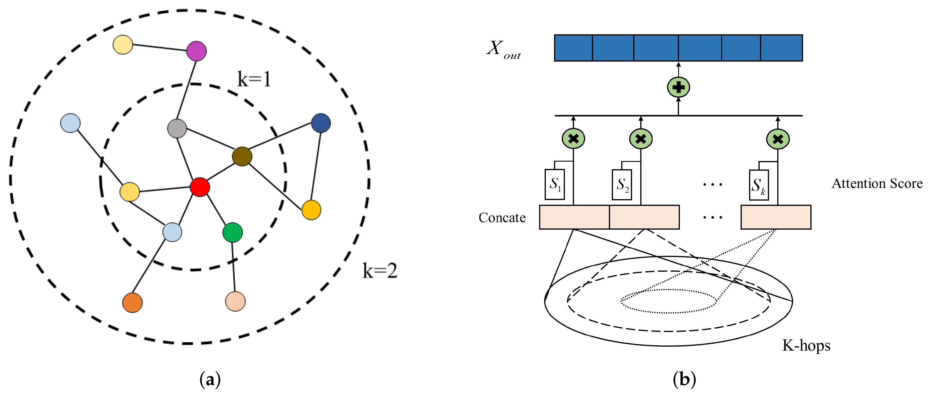
3.4. Adaptive Graph Convolution Module

A graph convolution network is widely adopted to process non-grid or unstructured data and aims to extract a high-level node feature representation through the neighborhood aggregation method. Li et al. [12] proposed a graph diffusion convolution layer to learn node representations by iteratively aggregating adjacent node features. For a k-layer diffusion model, the l-th layer information propagation step can be formulated as:

$$H^{\left(l\right)}=\widehat{A}{H}^{(l-1)}{W}^{\left(l\right)},$$

(7)

where $H^{\left(l\right)}\in R^{N\times d_l}$ denotes the output of node features of layer l, $H^{\left(0\right)}$ represents the initialized node feature, $\widehat{A}$ denotes the normalized adjacency matrix, and $W^{\left(l\right)}\in R^{d_{l-1}\times d_l}$ denotes the layer-specific model weight matrix.

However, a common challenge faced by graph convolution operation is that the node hidden states will become more similar when graph convolution layers go deeper. On the other hand, a shallow graph convolution network cannot sufficiently propagate the edge node information to the entire graph. Depending on the application, an appropriate receptive field or neighborhood size should be more desirable. To achieve this, motivated by [25], we explore an adaptive attention mechanism that can adaptively adjust the neighborhood size of each node. As shown in Figure 3, compared to simply concatenating $[H^{\left(0\right)},H^{\left(1\right)},\dots ,H^{\left(k\right)}]$ to combine different layers, the mechanism can maintain a better balance between local and global information propagation, which leads to more discriminative node features. The mechanism formula is as follows:

$$\begin{array}{cccc}\hfill & H^{\left(0\right)}=MLP\left(X\right),\hfill & \hfill \in & R^{N\times D}\hfill \\ \hfill & H^{\left(l\right)}=\alpha H^{\left(0\right)}+(1-\alpha )\widehat{A}{H}^{(l-1)},\hfill & \hfill \in & R^{N\times D}\hfill \\ \hfill & P=stack(H^{\left(0\right)},H^{\left(1\right)}\dots ,H^{\left(k\right)}),\hfill & \hfill \in & R^{N\times (k+1)\times D}\hfill \\ \hfill & S=reshape\left(\sigma \right(PW\left)\right),\hfill & \hfill \in & R^{N\times 1\times (k+1)}\hfill \\ \hfill & Z=squeeze\left(SP\right),\hfill & \hfill \in & R^{N\times D}\hfill \end{array}$$

(8)

where $H^{\left(0\right)}$ denotes the feature matrix derived from applying $MLP$ to the initialized node features X, W represents the trainable model parameters, and S represents the attention score for each layer. $\sigma$ denotes the activation function and we employ sigmoid here. $\alpha$ is a hyperparameter that controls the original node feature retention rate to preserve the local property.

To explore the interaction between global spatial adaptability and local dynamics, we apply static and dynamic graph structures to the adaptive graph convolution layer separately, i.e., replacing $\widehat{A}$ with learned $A_s$ and $A_d$. The final output is as follows:

$$Z=Z_{static}+Z_{dynamic}.$$

(9)

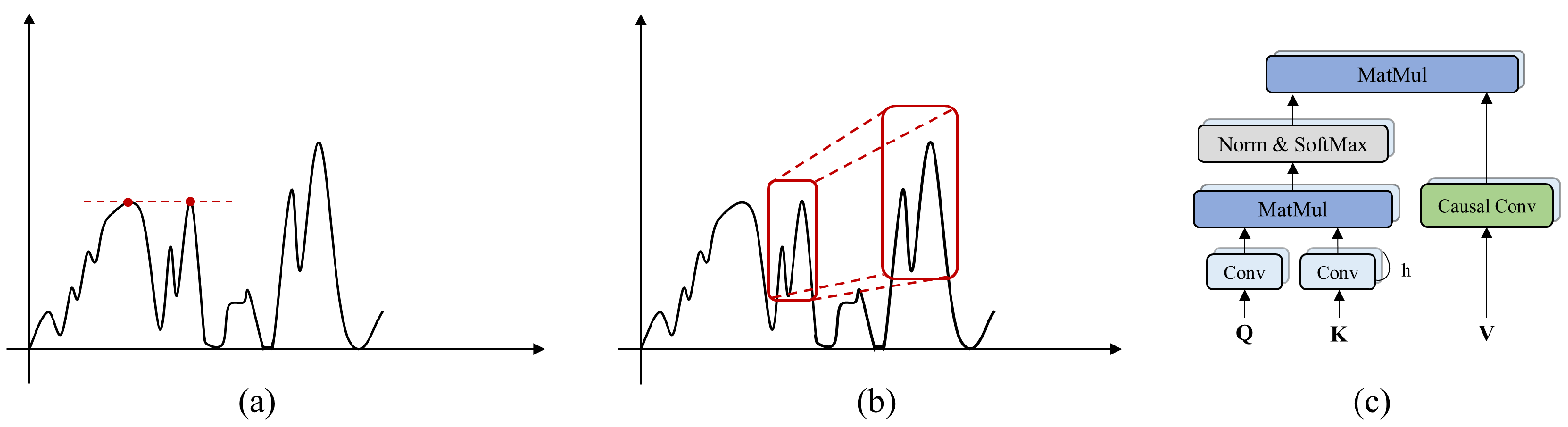
3.5. Gated Temporal Attention Module

The temporal attention module applies attention mechanisms to extract long-term temporal dependencies. As shown in Figure 2, this module consists of two parallel temporal attention layers, where the causal-trend attention mechanism is proposed. One layer is followed by a tangent hyperbolic activation function, which works as a filter. The other layer is followed by a sigmoid activation function as a gate, which controls the information that needs to be passed to the next module.

Multi-head self-attention [26] can effectively attend to information from different representation subspaces. The basic operation in multi-head self-attention has been defined in Equation (1), where all the keys, values, and queries are the same sequence representation, i.e., $\mathbf{Q}=\mathbf{K}=\mathbf{V}$. It first linearly projects the queries, keys, and values to different feature subspaces and then the attention function is performed in parallel. Lastly, the outputs are concatenated and once projected again. Formally, the final value can be defined as:

$$\begin{array}{c}\hfill \mathrm{MultiHead}(\mathbf{Q},\mathbf{K},\mathbf{V})=\oplus ({head}_1,\dots ,{head}_h)W^o\\ \hfill {head}_j=\mathrm{Attention}(\mathbf{Q}{W_j}^Q,\mathbf{K}{W_j}^K,\mathbf{V}{W_j}^V),\end{array}$$

(10)

where ${W_j}^Q,{W_j}^K,{W_j}^V$ are the projection matrices applied to $\mathbf{Q},\mathbf{K},\mathbf{V}$, $W^o$ is the output projection matrix, and the subscript h represents the number of attention heads. The multi-head self-attention can selectively focus on important information and efficiently explore the correlation between arbitrary elements in the sequence, thus leading to a flexible global receptive field.

Note that the attention mechanism was originally proposed to process discrete word sequences and it fails to learn the causality and local trends inherent in time series. The traditional attention mechanism may incorrectly match two points in the sequence because they are numerically similar. However, two points will exhibit significantly different local trends (e.g., uptrend or downtrend). Inspired by ASTGNN [27], we introduce a causal-trend attention mechanism to explore traffic series’ temporal property, as shown in Figure 4. To take local contextual information into consideration, we replace the projection operation on the queries and keys with 1D convolution. For masking future information, we employ causal convolution [28] on the values. Contextual information is taken as input and future information will not be intercepted, thus eventually benefiting the entire model to be aware of local changes and effectively fit predicted values. Formally, our causal-trend attention mechanism is defined as follows:

$$\begin{array}{c}\hfill \mathrm{CTAttention}(\mathbf{Q},\mathbf{K},\mathbf{V})=\oplus ({head}_1,\dots ,{head}_h)W^o\\ \hfill {head}_j=\mathrm{Attention}(\mathbf{Q}·{\mathrm{\Phi }}_j^Q,\mathbf{K}·{\mathrm{\Phi }}_j^K,\mathbf{V}·{\mathrm{\Psi }}_j^V),\end{array}$$

(11)

where ${\mathrm{\Phi }}_j^Q,{\mathrm{\Phi }}_j^K$ are 1D convolution kernel parameters and ${\mathrm{\Psi }}_j^V$ represents causal convolution kernel parameter.

3.6. Extra Components

In this section, we introduce extra components that the SATGCN adopts to enhance its representation power.

3.6.1. Spatial–Temporal Embedding

Though our method can capture spatial and temporal dynamic properties through separate modules, we ignore the spatioemporal heterogeneity and intrinsic signal order. Inspired by STSGCN [14], we equip position embedding into the model so that we can take into account both spatial and temporal information, which can enhance the ability to model spatial–temporal correlations. For the traffic signal sequence $X_G\in R^{N\times T\times C}$, we create a learnable temporal embedding matrix $T_E\in R^{T\times C}$ and spatial embedding matrix $S_E\in R^{N\times C}$. After the training phase, the embedding matrix will contain extra spatial–temporal information to improve the prediction performance.

We add the embedding matrix to the input traffic signal sequence with broadcasting operation for augmenting sequence representation:

$$X_{G+Temb+Semb}=X_G+T_E+S_E,$$

(12)

3.6.2. Loss Function

Compared with most current approaches, we learn the graph structure and optimize model parameters by minimizing a hybrid loss function that combines graph regularization loss and prediction loss. The hybrid loss function is as follows:

$$L(Y,\widehat{Y})=L_G+L1loss(Y,\widehat{Y}).$$

(13)

where $Y,\widehat{Y}$ denote the ground truth and predictions of the model, $L1loss$ is computed for back-propagation, and graph regularization loss $L_G$ is formulated following Equation (5).

4. Experiments

4.1. Datasets

We verify the performance of STAGCN on four public traffic network datasets, PEMS03, PEMS04, PEMS07, and PEMS08, collected from the Caltrans Performance Measurement System (PEMS).

PEMSD3: The dataset records the highway traffic flow information in the North Central Area. There are 358 road detectors placed in different regions, and the data were collected from 1 September 2018 to 30 November 2018.

PEMSD4: The dataset contains traffic flow data in the San Francisco Bay Area. We select 307 road detectors and capture the data from 1 January 2018 to 28 February 2018.

PEMSD7: The dataset refers to the traffic information collected from 883 loop detectors on Los Angeles County highways from 1 May 2017 to 31 August 2018.

PEMSD8: The dataset includes the traffic flow information in the San Bernardino area. It is gathered from 170 road detectors within the period from 1 July 2016 to 31 August 2016.

These datasets record traffic flow statistics on the highways of California and are aggregated into 5-min windows, which means that the sequence has 12 time steps in one hour. We utilize the historical data for the 12 time steps (1 h) to predict traffic flow for the next hour. In addition, we employ the same data pre-processing measures as STSGCN, and the data are normalized via the Z-score method. Further detailed dataset statistical information is provided in

Table 1. Dataset statistics.

Datasets	Samples	Nodes	Time Range
PEMS03	26,208	358	1 September 2018–30 November 2018
PEMS04	16,992	307	1 January 2018–28 February 2018
PEMS07	28,224	883	1 May 2017–31 August 2017
PEMS08	17,856	170	1 July 2016–31 August 2016

.

4.2. Experimental Setting

We split all datasets with ratio 6:2:2 into training sets, validation sets, and testing sets [29]. We use Equation (8) for the graph convolution operation and diffusion step $k=3$. The size of the hidden state is set to 64, and the dimension of node embeddings is set to 32. The number of attention heads is set to 8, and early stopping is employed to avoid overfitting. In addition, we train our model using the Adam optimizer [30] with an initial learning rate of 0.001. We choose mean absolute error (MAE), root mean squared error (RMSE), and mean absolute percentage error (MAPE) to evaluate the performance of our model. The evaluation metrics’ formulas are as follows:

(1) Mean absolute error (MAE):

$$\mathrm{MAE}=\frac{1}{n}\sum _{t=1}^n|Y_t-{\widehat{Y}}_t|,$$

(14)

MAE represents the average absolute difference between the predicted values and the ground truth. The smaller the MAE value, the better the prediction performance.

(2) Root mean square error (RMSE):

$$\mathrm{RMSE}=\sqrt{\frac{1}{n}\sum _{t=1}^n{(Y_t-{\widehat{Y}}_t)}^2},$$

(15)

RMSE describes how far predictions fall from measured true values using Euclidean distance. It is mainly used to evaluate the prediction error.

(3) Mean absolute percentage error (MAPE):

$$\mathrm{MAPE}=\frac{1}{n}\sum _{t=1}^n\left|\frac{Y_t-{\widehat{Y}}_t}{Y_t}\right|.$$

(16)

MAPE measures the prediction accuracy as a percentage and works best if the data have no extreme values.

4.3. Baseline Methods

• SVR: Support vector regression [31], which uses a support vector machine for prediction tasks.
• FC-LSTM: LSTM encoder–decoder predictor model, which employs a recurrent neural network with fully connected LSTM hidden units [32].
• DCRNN: Diffusion convolutional recurrent neural network [12], which integrates diffusion graph convolution into gated recurrent units.
• STGCN: Spatio–temporal graph convolutional network [33], which adopts graph convolutional and causal convolutional layers to model spatial and temporal dependencies.
• ASTGCN (r): Attention-based spatial-temporal graph convolutional network [34], which designs a spatiotemporal attention mechanism for traffic forecasting. It ensembles three different components to model the periodicity of traffic data, and we only use its recent input segment for a fair comparison.
• STSGCN: Spatial–temporal synchronous graph convolutional network [14], which captures correlations directly through a localized spatial–temporal graph.
• AGCRN: Adaptive graph convolutional recurrent network [35], which captures the node-specific spatial and temporal dynamics through a generated adaptive graph.
• STFGNN: Spatial–temporal fusion graph neural networks [36], which use the dynamic time warping algorithm (DTW) for graph construction to explore local and global spatial correlations.

4.4. Experimental Results

Table 2. Performance comparison of different methods on PEMS datasets.

Datasets	Metrics	SVR	FC-LSTM	DCRNN	STGCN	ASTGCN(r)	STSGCN	AGCRN	STFGCN	STAGCN
PEMS03	MAE	21.97	21.33	18.18	17.49	17.69	17.48	15.98	16.77	15.40
	MAPE(%)	21.51	23.33	18.91	17.15	19.40	16.78	15.23	16.30	14.48
	RMSE	35.29	35.11	30.31	30.12	29.66	29.21	28.25	28.34	26.23
PEMS04	MAE	28.70	27.14	24.70	22.70	22.93	21.19	19.83	19.83	19.02
	MAPE(%)	19.20	18.20	17.12	14.59	16.56	13.90	12.97	13.02	12.46
	RMSE	44.56	41.59	38.12	35.55	35.22	33.65	32.30	31.88	30.75
PEMS07	MAE	32.49	29.98	25.30	25.38	28.05	24.26	22.37	22.07	21.10
	MAPE(%)	14.26	13.20	11.66	11.08	13.92	10.21	9.12	9.21	8.92
	RMSE	50.22	45.94	38.58	38.78	42.57	39.03	36.55	35.80	34.10
PEMS08	MAE	23.25	22.20	17.86	18.02	18.61	17.13	15.95	16.64	15.36
	MAPE(%)	14.64	14.20	11.45	11.40	13.08	10.96	10.09	10.60	9.80
	RMSE	36.16	34.06	27.83	27.83	28.16	26.80	25.22	26.22	24.32

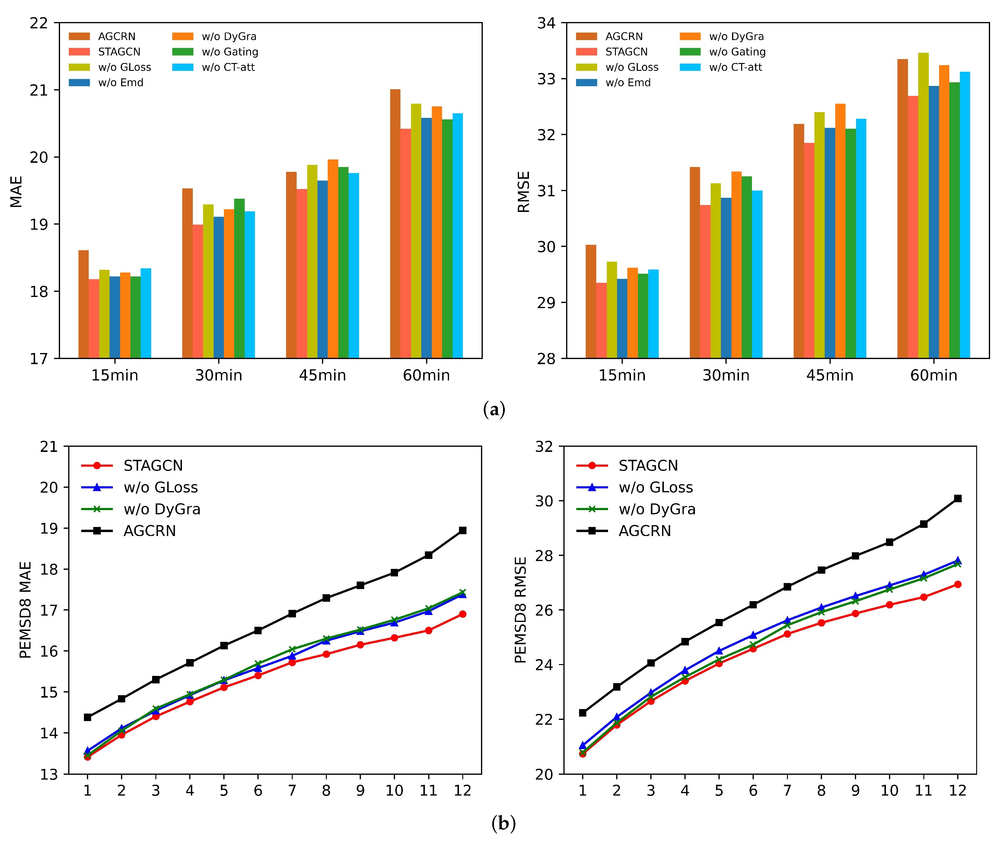
The best results are in bold and underline denotes re-implementation or re-training.

quantitatively presents the performance of our network on the PEMS datasets compared to other representative methods. STAGCN obtains superior performance with overall accuracy. We can observe that (1) SVR and FC-LSTM only take temporal correlations into consideration and ignore the spatial dependencies in road networks. Therefore, their performance is the worst. Especially, as shown in Table 2, SVR and FC-LSTM drop significantly on the PEMS04 and PEMS07 datasets with more detection nodes. GCN-based networks consistently outperform SVR and LSTM, demonstrating that graph convolution can effectively capture spatial heterogeneity in time series. For instance, urban and rural traffic flows have similar trend fluctuations during rush hours, but urban traffic is significantly higher than rural traffic. (2) Adaptive graph network AGCRN surpasses pre-defined graph models including DCRNN, ASTGCN, and STGCN by a large margin, indicating that data-driven spatial dependency modeling plays an integral role in traffic forecasting tasks. In most cases, the predefined graph is not optimal and struggles to adapt to complex spatiotemporal traffic data. Compared with the predefined graph structure, the learned adaptive graph matrix can uncover unseen graph structures automatically from the data, without any guidance of prior knowledge. (3) Compared to other graph-based works, STAGCN achieves superior performance, especially on the RMSE metric, for all datasets. We argue that our static–dynamic graph learning layer significantly improves the capability to capture local changing spatial heterogeneity and global spatial dependencies. The spatial dependencies between different locations are highly dynamic, which is determined by real-time traffic conditions and road networks. All the above baseline methods fail to model this dynamic attribute of the traffic network, restricting the prediction performance. (4) DCRNN and AGCRN are the typical RNN-based traffic forecasting works. Limited by the capability to model long-term temporal dependencies, their forecasting accuracy is much lower than our method. CNN-based forecasting works such as STGCN employ 1D convolution or TCN for temporal dependencies. Similar to the RNN-based works, it cannot effectively capture long-term temporal dependencies due to the size of the convolution kernel. Compared with RNN and CNN-based works, our temporal modeling layer based on the causal-trend attention mechanism can mitigate prediction error propagation to some extent, and further improve the prediction accuracy.

4.5. Ablation Study

To further investigate the effectiveness of different components that contribute to the superior performance of our model, we conduct ablation studies on the PEMS4 and PEMS8 datasets. We name the models without different components as follows:

• w/o GLoss: STAGCN without graph regularization loss.
• w/o Emb: STAGCN without spatial and temporal embedding.
• w/o DyGra: STAGCN without dynamic graph learning layer. We only use a static graph learning layer to adaptively model spatial correlation.
• w/o Gating: STAGCN without gating mechanism. We pass the output of the temporal attention layer to the next module directly without information selection.
• w/o CT-Att: STAGCN without causal-trend attention. We use traditional multi-head self-attention to replace causal-trend attention without considering local trends.

The evaluation results measured using MAE and RMSE are shown in Figure 5. We notice that STAGCN obtains the best result, indicating that different components of our model worked. In addition, some observations from these results deserve to be highlighted:

• As Figure 5a illustrates, removing graph regularization loss diminishes the performance significantly. This is because the graph loss function could optimize the adaptive traffic graph structure and facilitate graph information propagation. If the graph regularization loss function is removed, the learned adaptive graph matrix will not effectively reflect global spatial correlations in the traffic network. The result also indirectly proves that global spatial dependency has significant impacts on prediction performance.
• After removing the dynamic graph learning layer, the performance of our model gradually deteriorates over the 12 prediction time steps, which is evident in RMSE for the PEMS4 dataset and MAE for the PEMS8 dataset. We conjecture that the reason is that the long-term spatial dependencies have changed significantly, and the global graph structure cannot perceive fine-grained local spatial information. Our dynamic graph can capture local changing spatial correlations and overcome this shortcoming.
• STAGCN without the causal-trend attention mechanism performs much worse than STAGCN, demonstrating that modeling the causality and local trends in time series has better prediction performance than the traditional multi-head self-attention mechanism. Furthermore, the spatiotemporal embedding and gated mechanism are also essential, as they can improve the prediction accuracy at each prediction horizon.

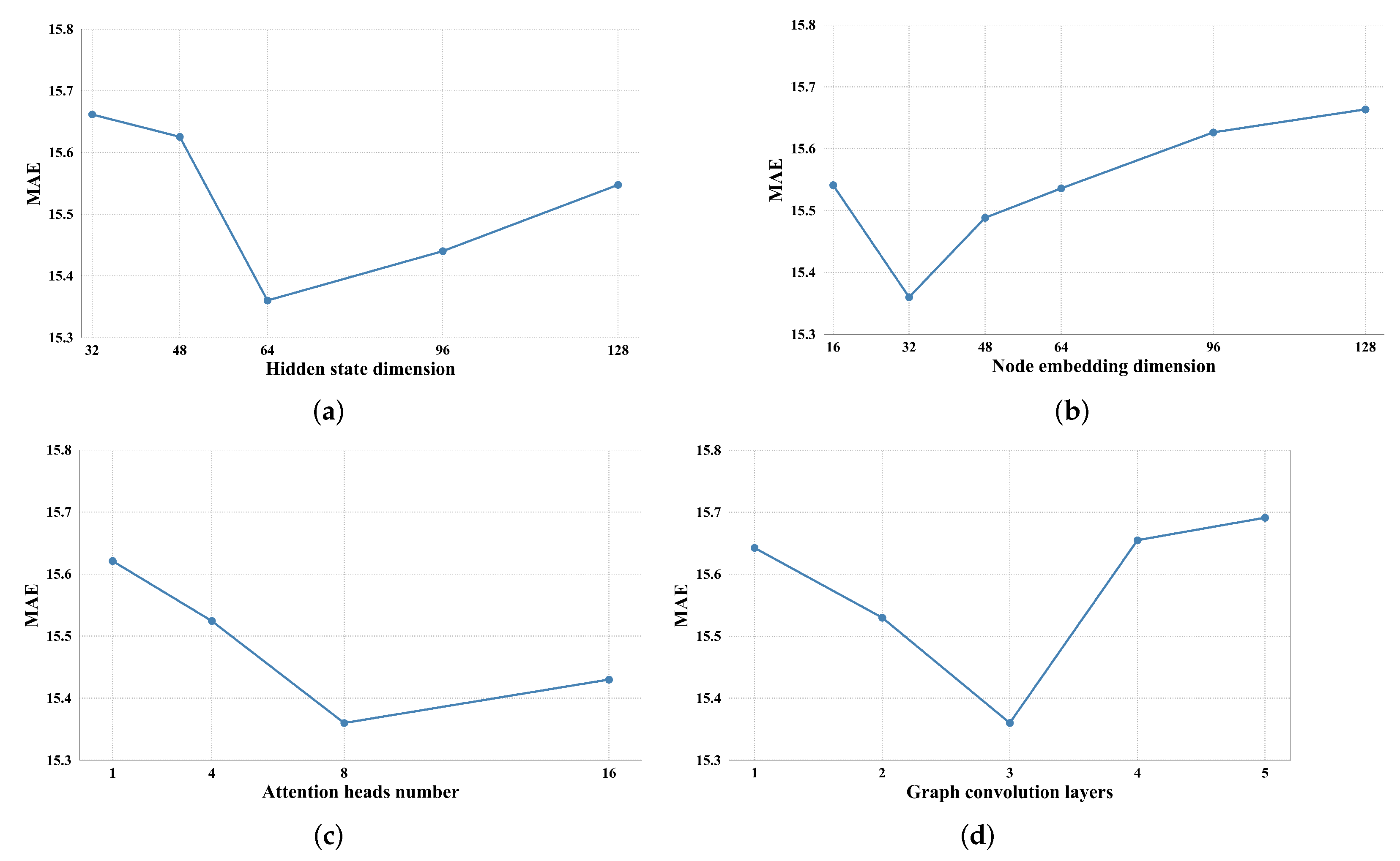
4.6. Parameter Study

To explore the influence of hyper-parameters, we conduct a hyper-parameter study on the core parameters of STAGCN. The chosen hyper-parameters are as follows: the dimension of hidden state and node embedding that range from 32 to 128 and 16 to 128, respectively, the layers of graph convolution, and the number of attention heads.

We repeat each experiment three times and report the average of MAE on the test set of PEMSD8. Figure 6 shows the experimental results of the parameter study. As shown in Figure 6a, though increasing the dimension of the hidden state can enhance the representation ability of sequence features and decrease the MAE loss, the overly high feature dimension will lead to overfitting, which diminishes the performance to a large extent. The optimal hidden state dimension is around 64. Compared with the hidden state dimension, increasing the node embedding dimension will only hamper the prediction performance. This is because the static graph structure is optimized by error back-propagation during the training phase, and an overly complex initialization graph structure and node embedding can make this optimization more difficult. As shown in Figure 6b, the model achieves superior performance with the dimension of node embedding at around 32. The result in Figure 6c indicates that increasing the number of attention heads is not cost-efficient in terms of model consumption and prediction performance when the number of attention heads is large. In addition, Figure 6d demonstrates the effect of graph convolution layers. The prediction performance is significantly improved when the number of layers ranges from 1 to 3, which indicates that a deeper graph convolution layer could effectively capture spatial dependencies in traffic data. However, the depth of the graph convolution layer should not be too high in case of overfitting.

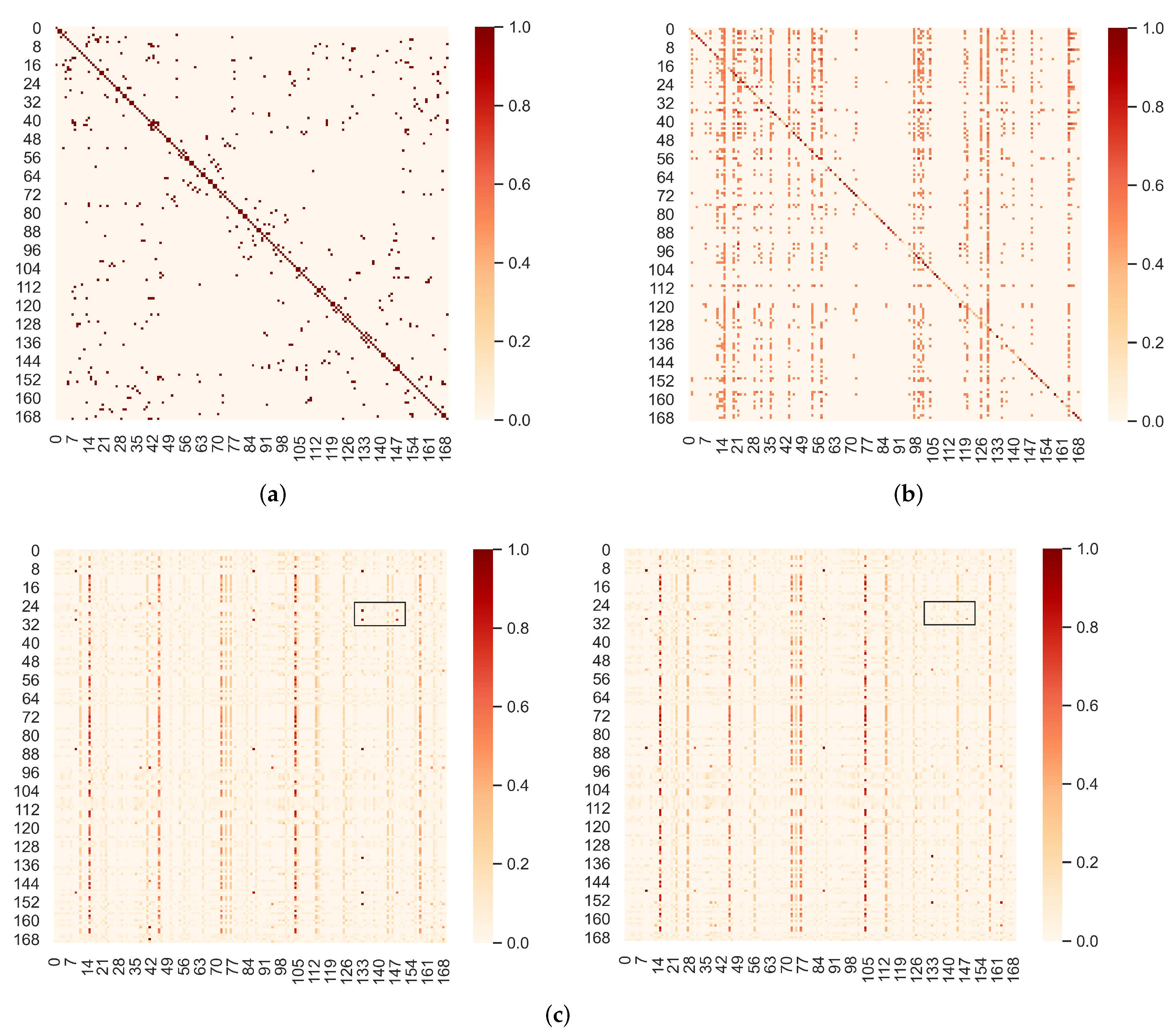
4.7. Effect of Graph Learning Layer

To verify the effectiveness of our proposed static graph learning layer, we conduct a study that experiments with different methods of constructing the static graph.

Table 3. Comparison of different static graph learning methods.

Methods	Graph Configuration	MAE	MAPE	RMSE
Predefined-A	$P_f$	16.26	10.19	25.27
Global-A	$A=Softmax\left(ReLU\right(W\left)\right)$	15.73	10.07	24.94
Directed-A	$A=Softmax\left(ReLU(E_1·{E_2}^T)\right)$	15.52	9.94	24.86
Ours	$A=Softmax\left(ReLU(tanh\left({\theta }_1{E}_1\right)·tanh\left({{\theta }_2}^T{E_2}^T\right))\right)$	15.36	9.80	24.32

The best results are in bold.

presents the experimental results with different forms of the static graph tested on the PEMS8 dataset. Predefined-A consists of road connectivity, where the values are 0 or 1. Global-A assumes that the static graph structure is a parameter matrix, which contains $N^2$ parameters. Directed-A is constructed directly with initialized node embeddings. In our method, a non-linear function layer is applied to node embeddings so that we can effectively compute similarity scores for node features. According to Table 3, our method achieves the lowest scores on all three evaluation matrices. It works even better than Predefined-A, Global-A, and Directed-A.

We further investigate the learned static adaptive graph via a visualization study. Figure 7a shows the predefined graph matrix in the PEMS8 dataset, Figure 7b shows the adaptive adjacency matrix learned by our model, and Figure 7c exhibits the dynamic graph structure learned on the two time-spans. As shown in Figure 7, we can observe that (1) in the predefined adjacency matrix, most nodes exhibit self-attention loop properties, i.e., diagonal line in the diagram. In contrast to manually defined self-attention loops, node self-attention in an adaptive graph is learned from spatial relationships in traffic data. (2) The predefined graph matrix is a symmetric matrix, which cannot process inflow and outflow information passed through each adjacent road. In our adaptive graph, most adjacent nodes have different connection weights, indicating that our model could capture road spatial interdependencies. (3) The dynamic graph structures are close to each other at different time intervals, demonstrating that the global space correlation appears to be stable in a short-term span. Furthermore, as marked with rectangular boxes in Figure 7c, the connectivity of local nodes is weakened in the short term, indicating that the proposed dynamic graph learning layer can effectively capture the changing correlations in local nodes. In order to better evaluate the performance of our model in practical application, we also visualize the predicted traffic flow of a certain node on the PEMSD8 dataset shown in Figure 8.

5. Conclusions

In this paper, we introduce a novel graph neural network for traffic forecasting. In contrast to most current methods that only concentrate on global spatial dependencies, our model captures global space adaptation and local dynamics in traffic data by constructing a static adaptive graph and dynamic graph from the data. A causal-trend attention mechanism is further introduced for long-term prediction tasks, which can effectively capture causality and local contextual information in time series. Extensive experiments on four public traffic network datasets demonstrate the superiority of our model over most existing methods. However, our model suffers from some inadequacies. For example, we argue that there should be information interaction between the static and dynamic graphs, and the two graph structures could complement each other. In the future, it would be worthwhile to explore the interaction between the static and dynamic graph structures and how to accelerate the inference speed of our proposed network. We will also attempt to apply our model to other multivariate time series forecasting tasks.

References

1. Huang, R.; Huang, C.; Liu, Y.; Dai, G.; Kong, W. LSGCN: Long Short-Term Traffic Prediction with Graph Convolutional Networks. In Proceedings of the Twenty-Ninth International Joint Conference on Artificial Intelligence, Yokohama, Japan, 11–17 July 2020; pp. 2355–2361. [Google Scholar]
2. Fang, Y.; Qin, Y.; Luo, H.; Zhao, F.; Zeng, L.; Hui, B.; Wang, C. CDGNet: A Cross-Time Dynamic Graph-based Deep Learning Model for Traffic Forecasting. arXiv 2021, arXiv:2112.02736. [Google Scholar]
3. Williams, B.M.; Hoel, L.A. Modeling and forecasting vehicular traffic flow as a seasonal ARIMA process: Theoretical basis and empirical results. J. Transp. Eng. 2003, 129, 664–672. [Google Scholar] [CrossRef] [Green Version]
4. Guo, J.; Huang, W.; Williams, B.M. Adaptive Kalman filter approach for stochastic short-term traffic flow rate prediction and uncertainty quantification. Transp. Res. Part C Emerg. Technol. 2014, 43, 50–64. [Google Scholar] [CrossRef]
5. Lim, B.; Zohren, S. Time-series forecasting with deep learning: A survey. Philos. Trans. R. Soc. A 2021, 379, 20200209. [Google Scholar] [CrossRef] [PubMed]
6. Wu, Z.; Pan, S.; Long, G.; Jiang, J.; Zhang, C. Graph WaveNet for Deep Spatial-Temporal Graph Modeling. In Proceedings of the IJCAI, Macao, China, 10–16 August 2019; pp. 1907–1913. [Google Scholar]
7. Wu, Z.; Pan, S.; Long, G.; Jiang, J.; Chang, X.; Zhang, C. Connecting the dots: Multivariate time series forecasting with graph neural networks. In Proceedings of the 26th ACM SIGKDD International Conference on Knowledge Discovery & Data Mining, Virtual Event, 6–10 July 2020; pp. 753–763. [Google Scholar]
8. Chen, Y.; Wu, L.; Zaki, M. Iterative deep graph learning for graph neural networks: Better and robust node embeddings. Adv. Neural Inf. Process. Syst. 2020, 33, 19314–19326. [Google Scholar]
9. Zhao, Z.; Chen, W.; Wu, X.; Chen, P.C.; Liu, J. LSTM network: A deep learning approach for short-term traffic forecast. IET Intell. Transp. Syst. 2017, 11, 68–75. [Google Scholar] [CrossRef] [Green Version]
10. Liu, Y.; Dong, H.; Wang, X.; Han, S. Time series prediction based on temporal convolutional network. In Proceedings of the 2019 IEEE/ACIS 18th International Conference on Computer and Information Science (ICIS), Beijing, China, 17–19 June 2019; pp. 300–305. [Google Scholar]
11. Yan, S.; Xiong, Y.; Lin, D. Spatial temporal graph convolutional networks for skeleton-based action recognition. In Proceedings of the Thirty-Second AAAI Conference on Artificial Intelligence, New Orleans, LA, USA, 2–7 February 2018; pp. 3482–3489. [Google Scholar]
12. Li, Y.; Yu, R.; Shahabi, C.; Liu, Y. Diffusion Convolutional Recurrent Neural Network: Data-Driven Traffic Forecasting. In Proceedings of the International Conference on Learning Representations, Vancouver, BC, Canada, 30 April–3 May 2018. [Google Scholar]
13. Wang, X.; Zhu, M.; Bo, D.; Cui, P.; Shi, C.; Pei, J. Am-gcn: Adaptive multi-channel graph convolutional networks. In Proceedings of the 26th ACM SIGKDD International Conference on Knowledge Discovery & Data Mining, Virtual Event, 6–10 July 2020; pp. 1243–1253. [Google Scholar]
14. Song, C.; Lin, Y.; Guo, S.; Wan, H. Spatial-temporal synchronous graph convolutional networks: A new framework for spatial-temporal network data forecasting. In Proceedings of the AAAI Conference on Artificial Intelligence, New York, NY, USA, 7–12 February 2020; Volume 34, pp. 914–921. [Google Scholar]
15. Kipf, T.N.; Welling, M. Semi-supervised classification with graph convolutional networks. In Proceedings of the International Conference on Learning Representations, Toulon, France, 24–26 April 2017. [Google Scholar]
16. Zhang, M.; Chen, Y. Link prediction based on graph neural networks. In Proceedings of the Advances in Neural Information Processing Systems, Montreal, QC, Canada, 3–8 December 2018; pp. 5165–5175. [Google Scholar]
17. Zhang, C.; Song, D.; Huang, C.; Swami, A.; Chawla, N.V. Heterogeneous graph neural network. In Proceedings of the 25th ACM SIGKDD International Conference on Knowledge Discovery &Data Mining, Anchorage, AK, USA, 4–8 August 2019; pp. 793–803. [Google Scholar]
18. Velickovic, P.; Cucurull, G.; Casanova, A.; Romero, A.; Lio, P.; Bengio, Y. Graph attention networks. Stat 2018, 1050, 4. [Google Scholar]
19. Li, G.; Muller, M.; Thabet, A.; Ghanem, B. Deepgcns: Can gcns go as deep as cnns? In Proceedings of the IEEE/CVF International Conference on Computer Vision, Seoul, Korea, 27–28 October 2019; pp. 9267–9276. [Google Scholar]
20. Wang, D.B.; Zhang, M.L.; Li, L. Adaptive graph guided disambiguation for partial label learning. IEEE Trans. Pattern Anal. Mach. Intell. 2021. [Google Scholar] [CrossRef] [PubMed]
21. Fukui, H.; Hirakawa, T.; Yamashita, T.; Fujiyoshi, H. Attention branch network: Learning of attention mechanism for visual explanation. In Proceedings of the IEEE/CVF conference on Computer Vision and Pattern Recognition, Seoul, Korea, 27–28 October 2019; pp. 10705–10714. [Google Scholar]
22. Yan, X.; Zheng, C.; Li, Z.; Wang, S.; Cui, S. Pointasnl: Robust point clouds processing using nonlocal neural networks with adaptive sampling. In Proceedings of the IEEE/CVF Conference on Computer Vision and Pattern Recognition, Seattle, WA, USA, 14–19 June 2020; pp. 5589–5598. [Google Scholar]
23. Zheng, C.; Fan, X.; Wang, C.; Qi, J. Gman: A graph multi-attention network for traffic prediction. In Proceedings of the AAAI Conference on Artificial Intelligence, New York, NY, USA, 7–12 February 2020; Volume 34, pp. 1234–1241. [Google Scholar]
24. Li, Z.; Zhang, G.; Xu, L.; Yu, J. Dynamic Graph Learning-Neural Network for Multivariate Time Series Modeling. arXiv 2021, arXiv:2112.03273. [Google Scholar]
25. Liu, M.; Gao, H.; Ji, S. Towards deeper graph neural networks. In Proceedings of the 26th ACM SIGKDD International Conference on Knowledge Discovery & Data Mining, Virtual Event, 6–10 July 2020; pp. 338–348. [Google Scholar]
26. Vaswani, A.; Shazeer, N.; Parmar, N.; Uszkoreit, J.; Jones, L.; Gomez, A.N.; Kaiser, Ł.; Polosukhin, I. Attention is all you need. In Proceedings of the Advances in Neural Information Processing Systems, Long Beach, CA, USA, 4–9 December 2017; Volume 30. [Google Scholar]
27. Guo, S.; Lin, Y.; Wan, H.; Li, X.; Cong, G. Learning dynamics and heterogeneity of spatial-temporal graph data for traffic forecasting. IEEE Trans. Knowl. Data Eng. 2021. [Google Scholar] [CrossRef]
28. Oord, A.V.D.; Dieleman, S.; Zen, H.; Simonyan, K.; Vinyals, O.; Graves, A.; Kalchbrenner, N.; Senior, A.; Kavukcuoglu, K. Wavenet: A generative model for raw audio. arXiv 2016, arXiv:1609.03499. [Google Scholar]
29. Demšar, J. Statistical comparisons of classifiers over multiple data sets. J. Mach. Learn. Res. 2006, 7, 1–30. [Google Scholar]
30. Kingma, D.P.; Ba, J. Adam: A Method for Stochastic Optimization. In Proceedings of the International Conference on Learning Representations, San Diego, CA, USA, 7–9 May 2015. [Google Scholar]
31. Drucker, H.; Burges, C.J.; Kaufman, L.; Smola, A.; Vapnik, V. Support vector regression machines. Adv. Neural Inf. Process. Syst. 1996, 9, 155–161. [Google Scholar]
32. Sutskever, I.; Vinyals, O.; Le, Q.V. Sequence to sequence learning with neural networks. In Proceedings of the Advances in Neural Information Processing Systems, Montreal, QC, Canada, 3–8 December 2014; Volume 27. [Google Scholar]
33. Yu, B.; Yin, H.; Zhu, Z. Spatio-Temporal Graph Convolutional Networks: A Deep Learning Framework for Traffic Forecasting. In Proceedings of the IJCAI, Stockholm, Sweden, 13–19 July 2018; pp. 3634–3640. [Google Scholar]
34. Guo, S.; Lin, Y.; Feng, N.; Song, C.; Wan, H. Attention based spatial-temporal graph convolutional networks for traffic flow forecasting. In Proceedings of the AAAI Conference on Artificial Intelligence, Honolulu, HI, USA, 27–28 January 2019; Volume 33, pp. 922–929. [Google Scholar]
35. Bai, L.; Yao, L.; Li, C.; Wang, X.; Wang, C. Adaptive graph convolutional recurrent network for traffic forecasting. Adv. Neural Inf. Process. Syst. 2020, 33, 17804–17815. [Google Scholar]
36. Li, M.; Zhu, Z. Spatial-temporal fusion graph neural networks for traffic flow forecasting. In Proceedings of the AAAI Conference on Artificial Intelligence, Virtually, 2–9 February 2021; Volume 35, pp. 4189–4196. [Google Scholar]
Figure 1. Example of spatiotemporal dependencies in PEMSD8 Dataset. (a) Global space correlation is dominated by the road network structure. (b) Sudden events, as marked with black boxes in the figure.
Mathematics 10 01599 g001
Figure 2. The framework of STAGCN. The model consists of a spatial static–dynamic graph learning layer, gated temporal attention module (Gated TAM), and adaptive graph convolution layer (GCN). The input and learned spatiotemporal embedding are first passed through Gated TAM, followed by the graph learning layer to obtain static and dynamic graphs. Then, feature representation and graphs are passed to GCN for spatial modeling.
Mathematics 10 01599 g002
Figure 3. An illustration of the proposed adaptive graph convolution module. This module can adaptively adjust the node neighborhood size according to the application. (a) K-hop neighbor nodes, (b) adaptive neighborhood size adjustment.
Mathematics 10 01599 g003
Figure 4. Comparison of traditional self-attention mechanism and our causal-trend attention mechanism. Traditional self-attention mechanisms may incorrectly match points in the sequence with similar values shown in (a). Our causal-trend attention mechanism is shown in (c), which replaces the projection operations with 1D and causal convolution. As shown in (b), such awareness of locality and causality in time series can correctly match the most relevant feature in the series.
Mathematics 10 01599 g004
Figure 5. Component analysis of STAGCN on two datasets. (a) Ablation study on PEMSD4, (b) performance comparison at each prediction horizon.
Mathematics 10 01599 g005
Figure 6. Parameter study on PEMSD8. (a) Effects of hidden state dimension, (b) effects of node embedding dimension, (c) effects of attention head number, (d) effects of graph convolution layers.
Mathematics 10 01599 g006
Figure 7. Graph structure visualization on PEMSD8. (a) Predefined graph structure, (b) learned adaptive adjacency matrix, (c) learned dynamic adjacency matrix at adjacent time intervals.
Mathematics 10 01599 g007
Figure 8. Visualization of the predicted values of traffic flow on the PEMSD8 dataset.
Mathematics 10 01599 g008