Thermoelastic Plane Waves in Materials with a Microstructure Based on Micropolar Thermoelasticity with Two Temperature and Higher Order Time Derivatives

Abstract

The study of the effect of the microstructure is important and is most evident in elastic vibrations of high frequency and short-wave duration. In addition to deformation caused by temperature and acting forces, the theory of micropolar thermoelasticity is applied to investigate the microstructure of materials when the vibration of their atoms or molecules is increased. This paper addresses a two-dimensional problem involving a thermoelastic micro-polar half-space with a traction-free surface and a known conductive temperature at the medium surface. The problem is treated in the framework of the concept of two-temperature thermoelasticity with a higher-order time derivative and phase delays, which takes into consideration the impact of microscopic structures in non-simple materials. The normal mode technique was applied to find the analytical formulas for thermal stresses, displacements, micro-rotation, temperature changes, and coupled stress. The numerical results are graphed, and the effect of the discrepancy indicator and higher-order temporal derivatives is examined. There are also some exceptional cases that are covered.

1. Introduction

In 1837, Duhamel established the coupled thermoelasticity theory that takes into account the constitutive relationship between the fields of heat and strain. Biot [1] introduced the model of coupled temperature elasticity, in which the basic equations were built using Fourier’s law, where the many theories of thermoelasticity were defined using the thermodynamics of irreversible processes. Based on this idea, the system governing the heat equation is of the parabolic type, which states that any thermal oscillation in a substance will affect all locations of the body instantly.

Several different models have been proposed by different researchers in the field of thermoelasticity to obtain hyperbolic heat conduction equations that allow finite velocities of heat waves. The first generalization in this context, known as “generalized LS theory”, was suggested by Lord and Shulman [2]. Green and Lindsey [3] proposed the GL model, which generalized the constitutive connections of stress and entropy by taking into account two alternative relaxation factors. Green and Naghdi [4,5,6] provided an additional extension of the theory of thermoelasticity as they proposed three new thermoelastic theories for homogeneous materials, termed GN models I, II and III. The dual-phase-delay theory (DPL), which was refined by Tzou [7,8,9], is the next extension of the thermoelastic theory. By incorporating dual-phase-lag into the heat flow and the temperature gradient, Tzou [7,8,9] constructed a foundational equation to describe the delayed performance of heat and mass transfer in different materials and microstructural factors such as phonon-electron interplay and phonon scattering.

Abouelregal [10,11,12,13,14] recently developed a set of new mathematical models that describe the heat transfer process in elastic bodies, involving higher-order time derivatives and phase delays (HOPL). These models are an extension of the mechanical frameworks for the heat transfer theories of Green-Naghdi [5,6] and Choudhuri [15] and heat transfer models with three-phase-delay (TPL) as well as Tzou [7,8,9] models. HOPL models provide a broad theoretical model of heat transfer with diverse microstructural interests, allowing researchers working in the field of heat transfer to reliably predict the thermal response of structures using a multiscale model.

The thermoelasticity model with two-temperature (2TT) was developed by Chen and Gurtin [16] and Chen et al. [17,18]. The Clausius–Duhem inequality was modified in this theory by a model based on two different temperatures: conductive and thermodynamic temperatures. The first was caused by a heat process, and the second was caused by a mechanical system that involves placing between the particles and the slabs of elastic material. They argued that the distinction between these three temperatures is proportional to the amount of heat supplied and that, in the absence of heat supply, the two temperatures are equal in a time-independent scenario. There are no differences between the two temperatures in simple substances and vice versa in the second category. The main difference between this theory and the classical one is the thermal dependence. One of the advantages of this model is that it describes the thermodynamic behavior better in thermoelastic problems that involve time-dependent heat sources, as the two temperatures are proportional to the heat source. In the case where the heat source is absent, the two temperatures are equal.

Quintanilla [19] discovered two-temperature thermoelasticity and described its existence, structural stability, convergence, and spatial behavior. Youssef [20] continued this concept based on the thermoelastic theory of heat transfer with a relaxation factor. In this regard, Abouelregal [10] also created a two-temperature modified thermoelastic version with higher-order time derivatives (HOPL) and three distinct phase delays. Ezzat and El-Karamany [21] developed a state space technique to provide a model of one-dimensional equations of two temperatures, extending magnetothermoelastic theory in a perfect electric conducting medium with two relaxation periods. Mukhopadhyay et al. expanded thermoelastic theory with two temperatures and dual-phase-lag in their paper [22]. In recent decades, researchers have devoted close attention to the concept of two-temperature thermoelasticity [23,24,25,26].

The micropolar elasticity theory, also known as the Cosserat elasticity theory or micropolar continuity mechanics, involves local point rotation in addition to the transformation assumed in the conventional model of elasticity, plus couple stress and force per unit area. In the conventional theory of elasticity, where there is no other type of stress, force stress is simply referred to as “stress”. The concept of couple stress can be traced back to Voigt’s early work on elasticity theory. Couple stress theories have recently been developed, utilizing the full range of current continuity mechanics possibilities. Because a drop in the stress concentration factor near holes and fractures is expected, generalized continuum concepts such as Cosserat elasticity are relevant to material performance. This can lead to increased hardness [27].

In recent years, Eringen’s theory of micropolar elasticity has attracted a lot of attention because of its potential value in examining the deformation characteristics of solids for which the conventional model is insufficient [28]. The micropolar concept is thought to be especially effective in studying materials made up of bar-like molecules with micro-rotational influences and the ability to sustain body and surface couples. A micropolar continuum is a compendium of linked particles that take the shape of tiny stiff bodies and move in both directions. The stress vector at a place on a body’s surface element entirely defines the force there [29]. Micropolarity has a substantial impact on all of the domains covered. Micropolarity has a diminishing influence on the magnitudes of all thermo-physical fields investigated.

The linear description of micropolar thermoelasticity was created by including the temperature influence into the concept of micropolar continua. The micropolar thermoelastic theory was established by Nowacki [30] and Eringen [31], who integrated thermal properties into the micropolar concept. Tauchert et al. [32] have developed the basic equations of the mathematical model of micropolar thermoelasticity. By studying the Green–Lindsay model, Dost and Tabarrok [33] were able to derive the equations for micropolar generalized thermoelasticity. Chandrasekharaiah [34] established an energy balance equation and a uniqueness theorem for anisotropic materials using a micropolar thermo elasticity model in which constitutive variables are dependent on heat flow. The constitutive foundations of the three-phase-lag theory of micropolar thermoelasticity were developed by El-Karamany and Ezzat [35]. They constructed a variational principle for a linear micropolar anisotropic and heterogeneous thermoelastic solid by proving the reciprocity and uniqueness theorems. Under the influence of mechanical plate stress, Alharbi et al. [36] proposed a mathematical model of a thermoelastic magnetic micropolar half-space with temperature-dependent material variables. Several comprehensive works have been presented that include the theory of micropolar thermoelasticity [37,38,39,40,41,42,43,44,45].

The main object of this investigation is to present a modified model of micropolar thermoelasticity with higher-order derivatives and dual-phase delay time. In addition to the proposed model incorporating microstructural influences in the heat transfer process, the macroscopic construction was also taken into account, with the assumption that the phonon–electron responses lead to a delay in the lattice temperature growth on the macroscopic scales. The proposed model was derived by applying the Taylor series expansions of Fourier’s law and the relationship between the two temperatures while maintaining conditions in phase lags and up to suitable higher orders.

The proposed model with phase lags is considered to be an extension of the two-temperature thermoelastic theory with one relaxation time [20] and a two-temperature model with two phase lags [22]. Through several previous studies, it has been realized that the concepts of dual-temperature thermoelasticity may be more applicable in real-world settings. As a result, it is expected that as the practical and theoretical study progresses, these generalized ideas of thermal elasticity with higher time derivatives will be revealed to be highly relevant to many technological applications and challenges.

The topic of wave propagation on the surface of an isotropic micropolar semi-space whose boundary is traction-free was investigated using the proposed model. The expressions for thermodynamic temperature, conductive temperature, microrotation, displacements, and thermal stresses are derived. For the purpose of comparison and investigation in the presented model, the distributions of the examined variables were estimated in tables and figures.

2. Mathematical Model and Basic Equations

In this section, field equations and constitutive relationships will be presented in a micropolar solid in the case of a thermal conductivity model with two temperature biphasic delays and higher-order time derivatives. The basic equations as presented by Eringen [31] in the absence of body forces, body couples, heat supply, and the balanced external force of the body take the following forms [46,47,48]:

The constitutive equations:

$${\sigma }_{ij}=\lambda {\epsilon }_{kk}{\delta }_{ij}+\left(\mu +\alpha \right){\epsilon }_{ij}+\mu {\epsilon }_{ji}-2\alpha {\epsilon }_{ijk}{\omega }_k-\gamma \theta {\delta }_{ij},$$

(1)

$$m_{ij}=\epsilon {\omega }_{k,k}{\delta }_{ij}+\left(\upsilon +\beta \right){\omega }_{j,i}+\left(\upsilon -\beta \right){\omega }_{i,j}.$$

(2)

$${\epsilon }_{ij}=\frac{1}{2}\left(u_{j,i}+u_{i,j}\right).$$

(3)

Here, ${\sigma }_{ij}$ is the stress tensor components, $u_i$ represents the displacement components, ${\omega }_k$ alludes to the components of the microrotation vector, $m_{ij}$ gives the components of the couple stress tensor, $\lambda$, $\mu$, $\alpha$ $\upsilon$, $\beta$ and $\epsilon$ are material constants, ${\delta }_{ij}$ is known as the Kronecker delta function, ${\epsilon }_{ij}$ describes the components of the electrode small stress tensor, ${\omega }_i$ shows the components of rotation, $\theta =T-T_0$ denotes the change in temperature above the reference temperature $T_0$ and $\gamma$ is the material constant given by $\gamma =\left(3\lambda +2\mu +\alpha \right){\alpha }_t$.

The equations of motion are given by:

$$i\ne j$$

$${\sigma }_{ij,j}=\rho {\stackrel{..}{u}}_i,$$

(4)

$${\epsilon }_{ijk}{\sigma }_{jk}+m_{ji,j}=\rho j{\stackrel{..}{\omega }}_{,i}i,j,k=1,2,3,$$

(5)

where ${\epsilon }_{ijk}$ is the permutation symbol, $\rho$ is the mass density and $j$ is micro-inertia.

Now, using the constitutive Equations (1) and (2), we can remove the stresses ${\sigma }_{ij}$ and $m_{ij}$ from the equations of motion (4) and (5) to obtain:

$$\left(\mu +\alpha \right){\nabla }^2\overrightarrow{\mathrm{u}}+\left(\lambda +\mu -\alpha \right)\nabla (\nabla .\overrightarrow{\mathrm{u}})+2\alpha \nabla \times \overrightarrow{\mathsf{\omega }}-\gamma \nabla \theta =\rho \frac{{\partial }^2\overrightarrow{\mathrm{u}}}{\partial t^2},$$

(6)

$$\left(\upsilon +\beta \right){\nabla }^2\overrightarrow{\mathsf{\omega }}+\left(\epsilon +\upsilon -\beta \right)\nabla (\nabla .\overrightarrow{\mathsf{\omega }})+2\alpha \nabla \times \overrightarrow{\mathrm{u}}-4\alpha \overrightarrow{\mathsf{\omega }}=\rho j\frac{{\partial }^2\overrightarrow{\mathsf{\omega }}}{\partial t^2}.$$

(7)

The energy equation can be written as:

$${\mathsf{\rho }\mathrm{C}}_{\mathrm{E}}\frac{\partial \mathsf{\theta }}{\partial \mathrm{t}}+{\mathsf{\gamma }\mathrm{T}}_0\frac{\partial }{\partial \mathrm{t}}(\mathrm{div}\overrightarrow{\mathrm{u}})=-\nabla .\overrightarrow{\mathrm{q}}+\mathsf{\rho }\mathrm{Q},$$

(8)

where $C_E$ is specific heat and $\overrightarrow{\mathrm{q}}$ is the heat flux vector. The conventional Fourier law can be written as:

$$\overrightarrow{\mathrm{q}}(\overrightarrow{\mathrm{x}},t)=-K\nabla \theta (\overrightarrow{\mathrm{x}},t),$$

(9)

where $\overrightarrow{\mathrm{x}}$ is the position vector and $K$ is the thermal conductivity.

A non-simple substance, according to Gurtin and Williams [17], is one in which the stress, energy, entropy, heat flow, and thermodynamic temperature at a given time all depend on the pasts of the deformation gradient, conduction temperature, and that temperature gradient up to that point.

Quintanilla [49,50] replaced the traditional Fourier law (9) as a consequence of the two-temperature concept to be in the form:

$$\overrightarrow{\mathrm{q}}(\overrightarrow{\mathrm{x}},t)=-K\nabla \phi (\overrightarrow{\mathrm{x}},t),$$

(10)

where $K$ denotes the thermal conductivity and $\phi$ represents the conductive temperature measured fulfils the relationship [16,17,18]:

$$\phi -\theta =a{\nabla }^2\phi ,$$

(11)

where $a>0$ is the two-temperature factor.

Quintanilla [20] and Mukhopadhyay et al. [22] developed the heat conduction with dual-phase-lag, which included a two-temperature model that took into account microstructural influences in the heat transmission process,

$$\overrightarrow{\mathrm{q}}(\overrightarrow{\mathrm{x}},t+{\tau }_q)=-K\nabla \phi (\overrightarrow{\mathrm{x}},t+{\tau }_{\phi }),$$

(12)

where ${\tau }_q$ and ${\tau }_{\phi }$ the phase delays of the heat flux and the conductive temperature gradient.

The expansion of the Taylor series for both sides of Equation (12) will be applied separately in the phase delays ${\tau }_q$, and ${\tau }_{\phi }$ until a sufficiently higher order of the $m$ and $n$ terms respectively [10,11]:

$$\left(1+{\displaystyle \sum }_{r=1}^m\frac{{\tau }_q^r}{r!}\frac{{\partial }^r}{\partial t^r}\right)\overrightarrow{\mathrm{q}}=-K\left(1+{\displaystyle \sum }_{r=1}^n\frac{{\tau }_{\phi }^r}{r!}\frac{{\partial }^r}{\partial t^r}\right)\nabla \phi .$$

(13)

If Equation (13) is combined with the energy Equation (8), we get the modified equation for higher order thermal conductivity with two temperatures as follows:

$$K\left(1+{\displaystyle \sum }_{r=1}^n\frac{{\tau }_{\phi }^r}{r!}\frac{{\partial }^r}{\partial t^r}\right){\nabla }^2\phi =\left(1+{\displaystyle \sum }_{r=1}^m\frac{{\tau }_q^r}{r!}\frac{{\partial }^r}{\partial t^r}\right)\left(\rho C_E\frac{\partial \theta }{\partial t}+\gamma T_0\frac{\partial }{\partial t}\left(\mathrm{div}\overrightarrow{\mathrm{u}}\right)-\rho Q\right).$$

(14)

The constraints on the thermomechanical parameters of an isotropic object satisfy the following inequalities:

$$3\lambda +2\mu >0,\mu >0,\mu +\alpha >0,\gamma +\epsilon >0,\alpha ,\gamma ,\epsilon >0.$$

(15)

Chirita et al. [51,52,53] show that there are certain limitations to the use of higher orders $m$ and $n$, such as when $m\ge 5$ produces an unstable system incapable of describing an actual physical aspect. However, when the approximation orders are less than or equal to four, the compliance with the Second Law of Thermodynamics must be investigated.

3. Particular Cases

From the modified higher order heat equation with two temperatures (14), it is possible to derive many models of thermoelasticity with two temperatures, both in the existence of the micropolar effect and in the absence of it. One-temperature thermoelastic models can also be derived.

Case 1:

In the absence of the micropolar influence, one/two-temperature thermoelastic theories can be obtained as follows:

• The conventional thermoelastic theory (CTE) [1] when ${\tau }_q={\tau }_{\phi }=0$, $a=0$,$\theta =\phi$;
• The Lord-Shulman generalized thermoelastic model (LS) [2] by setting ${\tau }_q={\tau }_0>0,$ $a=0$, $\theta =\phi$, ${\tau }_{\theta },{\tau }_{\phi }\to 0$ and taken $m=1$;
• The dual-phase-lag thermoelastic theory (DPL) [8,9] when $a=0$, ${\tau }_q,{\tau }_{\phi }>0$, $n=1$, and $m=2$;
• The dual-phase-lag two-temperature thermoelastic model (2DPL) [22] if $a>0$, ${\tau }_{\theta }={\tau }_{\phi }$, $m=n=1$;
• The generalized two-temperature model with one relaxation time (2LS) [20] if $a>0$, ${\tau }_{\phi }=0$, ${\tau }_q={\tau }_0>0,$ $m=n=1$;
• The generalized dual-phase-lag two-temperature thermoelastic model with high-order (2HDPL) [10] is obtained when $a>0$, ${\tau }_q,{\tau }_{\phi }>0$, $n,m\ge 1$;
• The generalized dual-phase-lag one-temperature thermoelastic model with high-order (1HDPL) [11] is obtained when $a=0$, ${\tau }_q,{\tau }_{\phi }>0$, $n,m\ge 1$.

Case 2:

In the case of a micropolar effect, one or two-temperature thermoelastic theories can also be obtained. It will be the same as in the previous cases, but the new models will be referred to with the same abbreviations with the addition of the letter “M” to them to become, respectively, 2MLS, 2MDPL, 2MHDPL, MTTLS, and MHTTE.

4. Problem Formulation

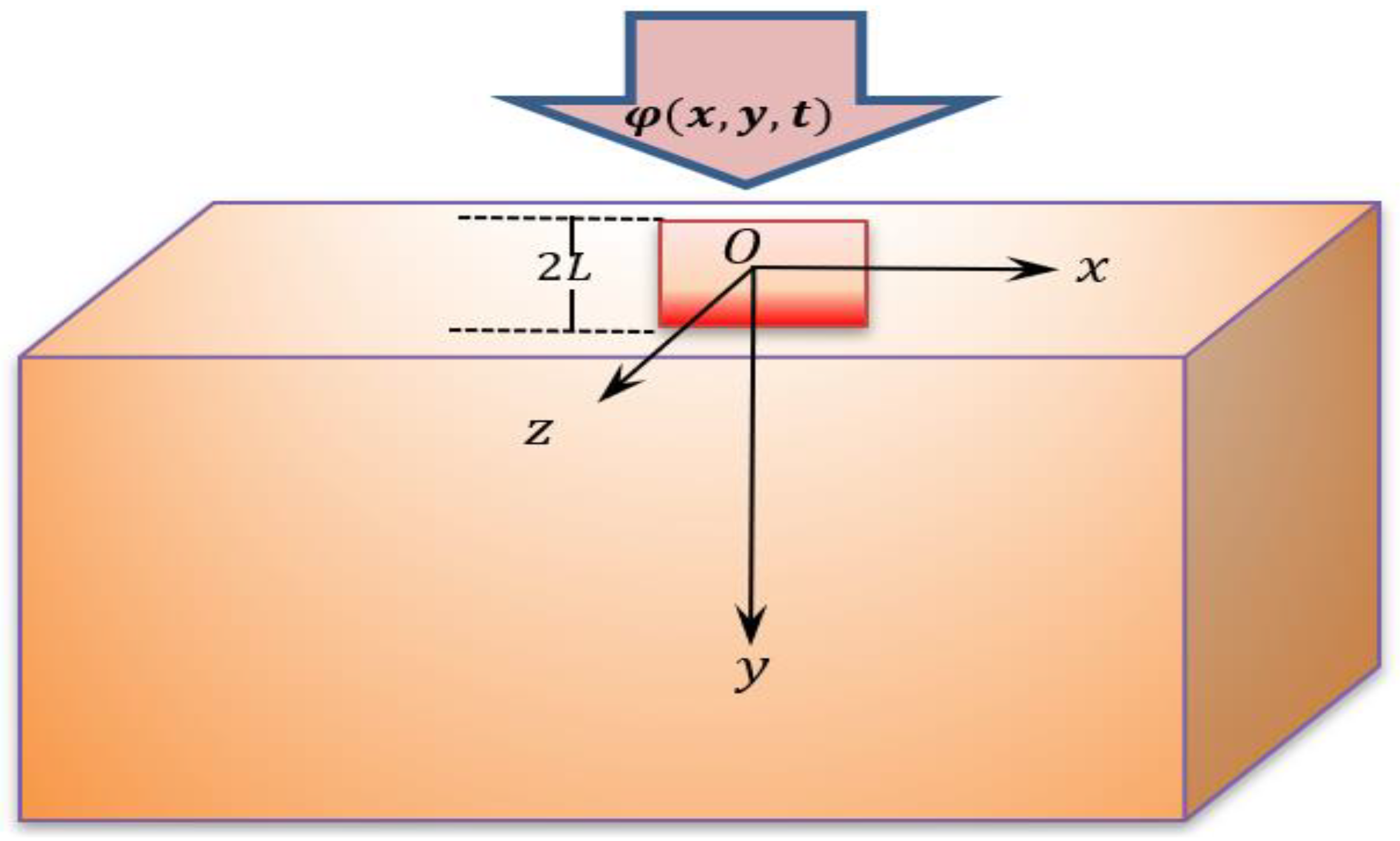
In this section, a half-space area of a micropolar homogeneous thermal material will be considered (see Figure 1). Initially, the medium is not deformed, uncompressed, and at a constant temperature of $T_0$. It was also hypothesized that the boundary of the medium $y=0$ is traction-free and exposed to a heat source, which would decrease over time and affect a small $2L$ bandwidth surrounding the $x$-axis. To study the problem, we will take the Cartesian coordinate system ($x,y,z$), provided that the origin of the coordinates is on the upper surface of the plane $y=0$, and the $y$-axis usually indicates the depth of the half-space. When considering plane waves in a plane, all particles on a line parallel to the $z$ axis are shifted equally. As a result, all considered fields are only functions of the $x$, $y$, and $t$ variables and do not depend on the $z$-coordinate. On the basis of these assumptions, the components of the displacement and microrotation vector will be in the following forms:

$$u_x=\left(x,y,t\right),u_y=v\left(x,y,t\right),u_z=0,\overrightarrow{\mathsf{\omega }}=\left(0,\omega ,0\right).$$

(16)

Then in $x$-$y$ plane, cubical dilatation $e$ can be written as:

$$e={\epsilon }_{kk}=\mathrm{div}\overrightarrow{\mathrm{u}}=\frac{\partial u}{\partial x}+\frac{\partial v}{\partial y}.$$

(17)

For two-dimensional problems, two equations for motion are obtained from Equation (6) and one for momentum balance from Equation (7) and can be expressed as follows:

$$\left(\lambda +\mu -\alpha \right)\frac{\partial e}{\partial x}+\left(\mu +\alpha \right){\nabla }^{2}u-\gamma \frac{\partial \theta }{\partial x}+2\alpha \frac{\partial \omega }{\partial y}=\rho \frac{{\partial }^{2}u}{\partial t^2},$$

(18)

$$\left(\lambda +\mu -\alpha \right)\frac{\partial e}{\partial y}+\left(\mu +\alpha \right){\nabla }^{2}v-\gamma \frac{\partial \theta }{\partial y}-2\alpha \frac{\partial \omega }{\partial x}=\rho \frac{{\partial }^{2}v}{\partial t^2},$$

(19)

$$\left(\upsilon +\beta \right){\nabla }^2\omega +2\alpha \left(\frac{\partial v}{\partial x}-\frac{\partial u}{\partial y}\right)-4\alpha \omega =\rho j\frac{{\partial }^2\omega }{\partial t^2}.$$

(20)

The higher order heat conduction Equation (14) with two temperatures can be expressed as:

$$K\left(1+{\displaystyle \sum }_{r=1}^n\frac{{\tau }_{\phi }^r}{r!}\frac{{\partial }^r}{\partial t^r}\right){\nabla }^2\phi =\left(1+{\displaystyle \sum }_{r=1}^m\frac{{\tau }_q^r}{r!}\frac{{\partial }^r}{\partial t^r}\right)\left(\rho C_E\frac{\partial \theta }{\partial t}+\gamma T_0\frac{\partial {\epsilon }_{kk}}{\partial t}\right).$$

(21)

In the $x$-$y$ plane, the constitutive relations (1) and (2) are:

$${\sigma }_{xx}=\left(\lambda +2\mu \right)\frac{\partial u}{\partial x}+\lambda \frac{\partial v}{\partial y}-\gamma \theta ,$$

(22)

$${\sigma }_{yy}=\left(\lambda +2\mu \right)\frac{\partial v}{\partial y}+\lambda \frac{\partial u}{\partial x}-\gamma \theta ,$$

(23)

$${\sigma }_{zz}=\lambda \left(\frac{\partial u}{\partial x}+\frac{\partial v}{\partial y}\right)-\gamma \theta ,$$

(24)

$${\sigma }_{xy}=\left(\mu +\alpha \right)\frac{\partial v}{\partial x}+\left(\mu -\alpha \right)\frac{\partial u}{\partial y}-2\alpha \omega ,$$

(25)

$${\sigma }_{yx}=\left(\mu -\alpha \right)\frac{\partial v}{\partial x}+\left(\mu +\alpha \right)\frac{\partial u}{\partial y}+2\alpha \omega ,$$

(26)

$$m_{zx}=\left(\upsilon -\beta \right)\frac{\partial \omega }{\partial x}=\left(\upsilon -\beta \right)m_{xz},$$

(27)

$$m_{zy}=\left(\upsilon -\beta \right)\frac{\partial \omega }{\partial y}=\left(\upsilon -\beta \right)m_{yz},$$

(28)

$$\phi -\theta =a{\nabla }^2\phi ,{\nabla }^2=\frac{{\partial }^2}{\partial x^2}+\frac{{\partial }^2}{\partial y^2}.$$

(29)

The above basic equations can be applied to any boundary condition problem. The micropolar thermoelastic semi-area with a traction-free surface exposed to a time-dependent decreasing heat source will be considered that affects a small $2L$-wide band inclosing the $x$-axis. Accordingly, the following boundary conditions will be taken into consideration:

• The mechanical boundary conditions:

  $${\sigma }_{yy}={\sigma }_{xy}=0\mathrm{a}ty=0,$$

  (30)

  $$m_{yz}=0\mathrm{a}ty=0.$$

  (31)
• Thermal boundary condition:

  $$\phi \left(x,y,t\right)={\phi }_{0}H\left(L-\left|x\right|\right)\exp \left(-bt\right)\mathrm{a}ty=0,$$

  (32)

  where ${\phi }_0$ is a constant and $H(.)$ is the known Heaviside unit step function. This relationship also indicates that the width of the applied thermal mechanical shock is $2L$ on the surface of the $x$-axis half space and its value is zero elsewhere.

5. Solution Methodology

For convenience, the following dimensionless quantities can be defined:

$$\begin{array}{c}\left\{x^{\prime },y^{\prime },u^{\prime },v^{\prime }\right\}=\frac{c_1}{\eta }\left\{x,y,u,v\right\},\left\{{\theta }^{\prime },{\phi }^{\prime }\right\}=\frac{\gamma }{\rho c_1^2}\left\{\theta ,\phi \right\},\left\{t^{\prime },{\tau }_q^{\prime },{\tau }_{\theta }^{\prime }\right\}=\frac{c_1^2}{\eta }\left\{t,{\tau }_q,{\tau }_{\theta }\right\}\\ {\sigma }_{ij}^{\prime }=\frac{{\sigma }_{ij}}{\alpha +\mu },m_{ij}^{\prime }=\frac{\alpha \eta m_{ij}}{c_1\left(\alpha +\mu \right)\left(\upsilon +\beta \right)},{\omega }^{\prime }=\frac{\alpha \omega }{\alpha +\mu },c_1^2=\frac{\left(\lambda +2\mu \right)}{\rho },\eta =\frac{k}{\rho C_E}.\end{array}$$

(33)

After eliminating primes for convenience in the nomenclature and using dimensionless forms (33), the motion and balance of momentum Equations (18)–(21) and the modified Equation (21) can be expressed as:

$${\beta }_1^2\frac{{\partial }^{2}u}{\partial x^2}+{\beta }_2^2\frac{{\partial }^{2}v}{\partial x\partial y}+\frac{{\partial }^{2}u}{\partial y^2}-{\beta }_1^2\frac{\partial \theta }{\partial x}+2\frac{\partial \omega }{\partial y}={\beta }_1^2\frac{{\partial }^{2}u}{\partial t^2},$$

(34)

$${\beta }_1^2\frac{{\partial }^{2}v}{\partial y^2}+{\beta }_2^2\frac{{\partial }^{2}u}{\partial x\partial y}+\frac{{\partial }^{2}v}{\partial x^2}-{\beta }_1^2\frac{\partial \theta }{\partial y}-2\frac{\partial \omega }{\partial x}={\beta }_1^2\frac{{\partial }^{2}v}{\partial t^2},$$

(35)

$${\nabla }^2\omega +g_1\left(\frac{\partial v}{\partial x}-\frac{\partial u}{\partial y}\right)-g_2\omega =g_3\frac{{\partial }^2\omega }{\partial t^2},$$

(36)

$$\left(1+{\displaystyle \sum }_{r=1}^n\frac{{\tau }_{\phi }^r}{r!}\frac{{\partial }^r}{\partial t^r}\right){\nabla }^2\phi =\left(1+{\displaystyle \sum }_{r=1}^m\frac{{\tau }_q^r}{r!}\frac{{\partial }^r}{\partial t^r}\right)\left(\frac{\partial \theta }{\partial t}+g\frac{\partial {\epsilon }_{kk}}{\partial t}\right),$$

(37)

where

$$\begin{array}{c}{\beta }_1^2=\frac{\lambda +2\mu }{\alpha +\mu },{\beta }_2^2=\left({\beta }_1^2-1\right),g_1=\frac{2{\alpha }^2{\eta }^2}{c_1^2\left(\alpha +\mu \right)\left(\upsilon +\beta \right)}\\ g_2=\frac{4\alpha {\eta }^2}{c_1^2\left(\upsilon +\beta \right)},g_3=\frac{\rho j{c}_1^2}{\upsilon +\beta },g=\frac{\eta {\gamma }^2{T}_0}{\rho c_1^{2}K}\end{array}.$$

(38)

In the same way, using the non-dimensional constitutive Equations (22)–(29), they become:

$${\sigma }_{xx}={\beta }_1^2\frac{\partial u}{\partial x}+{\delta }_2\frac{\partial v}{\partial y}-{\beta }_1^2\theta ,$$

(39)

$${\sigma }_{yy}={\beta }_1^2\frac{\partial v}{\partial y}+{\delta }_2\frac{\partial u}{\partial x}-{\beta }_1^2\theta ,$$

(40)

$${\sigma }_{zz}={\delta }_2\left(\frac{\partial u}{\partial x}+\frac{\partial v}{\partial y}\right)-{\beta }_1^2\theta ,$$

(41)

$${\sigma }_{xy}=\frac{\partial v}{\partial x}+{\delta }_3\frac{\partial u}{\partial y}-2\omega ,$$

(42)

$${\sigma }_{yx}=\frac{\partial u}{\partial x}+{\delta }_3\frac{\partial v}{\partial y}+2\omega ,$$

(43)

$$m_{zx}={\delta }_4\frac{\partial \omega }{\partial x}={\delta }_4{m}_{xz},$$

(44)

$$m_{zy}={\delta }_4\frac{\partial \omega }{\partial y}={\delta }_4{m}_{yz},$$

(45)

$$\phi -\theta =a_1{\nabla }^2\phi ,$$

(46)

where

$${\delta }_2=\frac{\lambda }{\alpha +\mu },{\delta }_3=\frac{\mu -\alpha }{\alpha +\mu },{\delta }_4=\frac{\upsilon -\beta }{\upsilon +\beta },a_1=\frac{c_1^2}{{\eta }^2}a.$$

(47)

Due to the large number of differential equations as well as field variables, the potential functions $\mathsf{\Phi }\left(x,y,t\right)$ and $\overrightarrow{\mathsf{\Psi }}\left(x,y,t\right)$ can be introduced, which are defined by the relations:

$$\overrightarrow{\mathrm{u}}=\nabla \mathsf{\Phi }+\nabla \times \overrightarrow{\mathsf{\Psi }},\overrightarrow{\mathsf{\Psi }}=\left(0,0,\mathsf{\Psi }\right).$$

(48)

Using the above relationship, the components of the displacement $u\left(x,y,t\right)$ and $v\left(x,y,t\right)$ can be expressed as:

$$u=\frac{\partial \mathsf{\Phi }}{\partial x}+\frac{\partial \mathsf{\Psi }}{\partial y},$$

(49)

$$v=\frac{\partial \mathsf{\Phi }}{\partial y}-\frac{\partial \mathsf{\Psi }}{\partial x}.$$

(50)

Entering (49) and (50) into (34)–(37) yields the following results:

$${\nabla }^2\left({\beta }_1^2\frac{\partial \mathsf{\Phi }}{\partial x}+\frac{\partial \mathsf{\Psi }}{\partial y}\right)-{\beta }_1^2\frac{\partial \theta }{\partial x}+2\frac{\partial \omega }{\partial y}={\beta }_1^2\frac{{\partial }^2}{\partial t^2}\left(\frac{\partial \mathsf{\Phi }}{\partial x}+\frac{\partial \mathsf{\Psi }}{\partial y}\right),$$

(51)

$${\nabla }^2\left({\beta }_1^2\frac{\partial \mathsf{\Phi }}{\partial y}-\frac{\partial \mathsf{\Psi }}{\partial x}\right)-{\beta }_1^2\frac{\partial \theta }{\partial y}-2\frac{\partial \omega }{\partial x}={\beta }_1^2\frac{{\partial }^2}{\partial t^2}\left(\frac{\partial \mathsf{\Phi }}{\partial y}-\frac{\partial \mathsf{\Psi }}{\partial x}\right),$$

(52)

$$\left({\nabla }^2-g_3\frac{{\partial }^2}{\partial t^2}-g_2\right)\omega =g_1{\nabla }^2\mathsf{\Psi },$$

(53)

$$\left(1+{\displaystyle \sum }_{r=1}^n\frac{{\tau }_{\phi }^r}{r!}\frac{{\partial }^r}{\partial t^r}\right){\nabla }^2\phi =\left(1+{\displaystyle \sum }_{r=1}^m\frac{{\tau }_q^r}{r!}\frac{{\partial }^r}{\partial t^r}\right)\left(\frac{\partial \theta }{\partial t}+g\frac{{\partial }^2}{\partial t^2}{\nabla }^2\mathsf{\Phi }\right).$$

(54)

Equations (51) and (52) can be simplified to the following equations.

$$\left({\nabla }^2-\frac{{\partial }^2}{\partial t^2}\right)\mathsf{\Phi }=\theta ,$$

(55)

$$\left({\nabla }^2-{\beta }_1^2\frac{{\partial }^2}{\partial t^2}\right)\mathsf{\Psi }=-2\omega .$$

(56)

6. Normal Mode Solution

To solve equations from (51) to (56), the solutions will be imposed as follows:

$$\left(\theta ,\phi ,u,v,{\sigma }_{ij},\mathsf{\Phi },m_{ij},\mathsf{\Psi },\omega \right)=\left(\overline{\theta },\overline{\phi },\overline{u},\overline{v},{\overline{\sigma }}_{ij},\overline{\mathsf{\Phi }},{\overline{m}}_{ij},\overline{\mathsf{\Psi }},\overline{\omega }\right)\left(y\right)\exp \left(i\zeta x+\mathsf{\Omega }t\right),$$

(57)

where $\mathsf{\Omega }$ denotes the complex constant angular frequency and $\zeta$ denotes the wave number along the $x$-axis. The variables $\overline{\theta }$, $\overline{\phi }$, $\overline{u}$, $\overline{v}$, ${\overline{\sigma }}_{ij}$, $\overline{\mathsf{\Phi }}$, $\overline{\mathsf{\Psi }}$ and $\overline{\omega }$ are indefinite amplitude functions in the variable $y$ only and are completely separate from the time $t$ and coordinate $x$.

Substituting Equation (57) in Equations (51)–(56), the following equations can be obtained:

$$\left(D^2-{\epsilon }_1\right)\overline{\mathsf{\Phi }}=\overline{\theta }$$

(58)

$$\left(D^2-{\zeta }^2\right)\overline{\phi }={\epsilon }_4\left(\overline{\theta }+g\left(D^2-{\zeta }^2\right)\overline{\mathsf{\Phi }}\right)$$

(59)

$$\overline{\phi }-\overline{\theta }=a_1\left(D^2-{\zeta }^2\right)\overline{\phi }$$

(60)

$$\left(D^2-{\epsilon }_2\right)\overline{\mathsf{\Psi }}=-2\overline{\omega }$$

(61)

$$\left(D^2-{\epsilon }_3\right)\overline{\omega }=g_1\left(D^2-{\zeta }^2\right)\overline{\mathsf{\Psi }},$$

(62)

where

$$\begin{array}{c}D=\frac{d}{dy},{\epsilon }_1={\zeta }^2+{\mathsf{\Omega }}^2,{\epsilon }_2={\zeta }^2+{\beta }_1^2{\mathsf{\Omega }}^2,{\epsilon }_3={\zeta }^2+g_2+g_3{\mathsf{\Omega }}^2,\\ {\epsilon }_4=\frac{\mathsf{\Omega }{L}_q}{L_{\phi }},L_q=1+{\displaystyle {\displaystyle \sum }_{r=1}^m}\frac{{\mathsf{\Omega }}^r{\tau }_q^r}{r!},L_{\phi }=1+{\displaystyle {\displaystyle \sum }_{r=1}^n}\frac{{\mathsf{\Omega }}^r{\tau }_{\phi }^r}{r!}.\end{array}$$

(63)

By removing $\overline{\theta }$, $\overline{\phi }$, $\overline{\mathsf{\Phi }}$ from Equations (58)–(60) and $\overline{\omega }$, $\overline{\mathsf{\Psi }}$ from Equations (61) and (62), we obtain:

$$\left(D^4-{\eta }_1{D}^2+{\gamma }_1\right)\left\{\overline{\theta },\overline{\phi },\overline{\mathsf{\Phi }}\right\}\left(y\right)=0,$$

(64)

$$\left(D^4-{\eta }_2{D}^2+{\gamma }_2\right)\left\{\overline{\omega },\overline{\mathsf{\Psi }}\right\}\left(y\right)=0,$$

(65)

where

$$\begin{array}{c}{\eta }_1=\frac{\left({\zeta }^2+{\epsilon }_1+{\epsilon }_4\left[a_1\left({\epsilon }_1+g{\zeta }^2)+\left(a_1{\zeta }^2+1\right)\left(g+1\right)\right)\right]\right)}{\left(a_1{\epsilon }_4\left(g+1\right)+1\right)},{\eta }_2={\epsilon }_2+{\epsilon }_3-g_{1,}\\ {\gamma }_1=\frac{\left({\zeta }^2{\epsilon }_1+{\epsilon }_4\left(a_1{\zeta }^2+1\right)\left({\epsilon }_1+g{\zeta }^2\right)\right)}{\left(a_1{\epsilon }_4\left(g+1\right)+1\right)},{\gamma }_2={\epsilon }_2{\epsilon }_3-2g_1{\zeta }^2.\end{array}$$

(66)

The solutions of Equations (64) and (65) fulfill the consistency criteria such that the functions $\overline{\theta }$, $\overline{\phi }$, $\overline{u}$, $\overline{v}$, ${\overline{\sigma }}_{ij}$, $\overline{\mathsf{\Phi }}$, $\overline{\mathsf{\Psi }}$ and $\overline{\omega }$ trend to zero as $y$ goes to infinity may be expressed as:

$$\overline{\mathsf{\Phi }}\left(y\right)={\displaystyle \sum }_{j=1}^2{A}_j{\mathrm{e}}^{-{\lambda }_{j}y},$$

(67)

$$\overline{\mathsf{\Psi }}\left(y\right)={\displaystyle \sum }_{j=1}^2{B}_j{\mathrm{e}}^{-{\mu }_{j}y},$$

(68)

$$\overline{\theta }\left(y\right)={\displaystyle \sum }_{j=1}^2{A}_j^{\prime }{\mathrm{e}}^{-{\lambda }_{j}y},$$

(69)

$$\overline{\phi }\left(y\right)={\displaystyle \sum }_{j=1}^2{A}_j^{″}{\mathrm{e}}^{-{\lambda }_{j}y},$$

(70)

$$\overline{\omega }\left(y\right)={{\displaystyle \sum }}_{j=1}^2{B}_j^{\prime }{\mathrm{e}}^{-{\mu }_{j}y},$$

(71)

where the parameters $A_j,$ $A_j^{\prime }$, $A_j^{″}$, $B_j$ and $B_j^{\prime }$,$\left(i=1,2,3\right)$ are some parameters depending on $\zeta$ and $\mathsf{\Omega }$. The parameters ${\lambda }_i,{\mu }_j,\left(i=1,2\right)$ are the positive roots of the equations:

$${\lambda }^4-{\eta }_1{\lambda }^2+{\gamma }_1=0,$$

(72)

$${\mu }^4-{\eta }_2{\mu }^2+{\gamma }_2=0.$$

(73)

Substituting Equations (67)–(71) into Equations (58)–(62), the following relations can be obtained:

$$A_j^{\prime }=\left({\lambda }_j^2-{\epsilon }_1\right)A_j,A_j^{″}=\frac{\left({\lambda }_j^2-{\epsilon }_1\right)}{1-a_1\left({\lambda }_j^2-{\zeta }^2\right)}{A}_j,B_j^{\prime }=-\frac{1}{2}\left({\mu }_j^2-{\epsilon }_2\right)B_j,j=1,2.$$

(74)

Introducing relations (74) into Equations (67)–(71), then we have:

$$\overline{\theta }={\displaystyle \sum }_{j=1}^2\left({\lambda }_j^2-{\epsilon }_1\right)A_j{\mathrm{e}}^{-{\lambda }_{j}y},$$

(75)

$$\overline{\phi }={\displaystyle \sum }_{j=1}^2\frac{{\lambda }_j^2-{\epsilon }_1}{1-a_1\left({\lambda }_j^2-{\zeta }^2\right)}{A}_j{\mathrm{e}}^{-{\lambda }_{j}y},$$

(76)

$$\overline{\omega }=-\frac{1}{2}{\displaystyle \sum }_{j=1}^2\left({\mu }_j^2-{\epsilon }_2\right)B_j{\mathrm{e}}^{-{\mu }_{j}y}.$$

(77)

To derive the displacement components $\overline{u}$ and $\overline{v}$, we first substitute Equation (57) into Equations (49) and (50) and then use Equations (67) and (68):

$$\overline{u}=i\zeta {\displaystyle \sum }_{j=1}^2{\lambda }_j{A}_j{\mathrm{e}}^{-{\lambda }_{j}y}-{\displaystyle \sum }_{j=1}^2{\lambda }_j{B}_j{\mathrm{e}}^{-{\mu }_{j}y},$$

(78)

$$\overline{v}=-{\displaystyle \sum }_{j=1}^2{\lambda }_j{A}_j{\mathrm{e}}^{-{\lambda }_{j}y}-i\zeta {\displaystyle \sum }_{j=1}^2{\lambda }_j{B}_j{\mathrm{e}}^{-{\mu }_{j}y}.$$

(79)

After applying the normal mode solution method, the thermal and couple stresses components ${\overline{\sigma }}_{ij}$ and ${\overline{m}}_{ij}$ can be written in the forms:

$${\overline{\sigma }}_{xx}={\displaystyle \sum }_{j=1}^2{\alpha }_{1j}{A}_j{\mathrm{e}}^{-{\lambda }_{j}y}+{\displaystyle \sum }_{j=1}^2{\beta }_{1j}{B}_j{\mathrm{e}}^{-{\mu }_{j}y},$$

(80)

$${\overline{\sigma }}_{yy}={\displaystyle \sum }_{j=1}^2{\alpha }_{2j}{A}_j{\mathrm{e}}^{-{\lambda }_{j}y}+{\displaystyle \sum }_{j=1}^2{\beta }_{2j}{B}_j{\mathrm{e}}^{-{\mu }_{j}y},$$

(81)

$${\overline{\sigma }}_{zz}={\displaystyle \sum }_{j=1}^2{\alpha }_{3j}{A}_j{\mathrm{e}}^{-{\lambda }_{j}y}+{\displaystyle \sum }_{j=1}^2{\beta }_{3j}{B}_j{\mathrm{e}}^{-{\mu }_{j}y},$$

(82)

$${\overline{\sigma }}_{xy}={\displaystyle \sum }_{j=1}^2{\alpha }_{4j}{A}_j{\mathrm{e}}^{-{\lambda }_{j}y}+{\displaystyle \sum }_{j=1}^2{\beta }_{4j}{B}_j{\mathrm{e}}^{-{\mu }_{j}y},$$

(83)

$${\overline{\sigma }}_{yx}={\displaystyle \sum }_{j=1}^2{\alpha }_{5j}{A}_j{\mathrm{e}}^{-{\lambda }_{j}y}+{\displaystyle \sum }_{j=1}^2{\beta }_{5j}{B}_j{\mathrm{e}}^{-{\mu }_{j}y},$$

(84)

$${\overline{m}}_{xz}=-\frac{i\zeta }{2}{\displaystyle \sum }_{j=1}^2\left({\mu }_j^2-{\epsilon }_2\right)B_j{\mathrm{e}}^{-{\mu }_{j}y},$$

(85)

$${\overline{m}}_{yz}=\frac{1}{2}{\displaystyle \sum }_{j=1}^2{\mu }_j\left({\mu }_j^2-{\epsilon }_2\right)B_j{\mathrm{e}}^{-{\mu }_{j}y},$$

(86)

where

$$\begin{array}{c}{\alpha }_{1j}=\left({\delta }_2-{\beta }_1^2\right){\lambda }_j^2+{\beta }_1^2{\epsilon }_1-{\zeta }^2{\beta }_1^2,{\beta }_{1j}=i\zeta {\mu }_j\left({\delta }_2-{\delta }_1\right),{\alpha }_{2j}={\beta }_1^2{\epsilon }_1-{\zeta }^2{\delta }_2,\\ {\beta }_{2j}=i\zeta {\mu }_j\left({\beta }_1^2-{\delta }_2\right),{\alpha }_{3j}=-{\beta }_1^2\left({\lambda }_j^2-{\epsilon }_1\right)-{\zeta }^2{\delta }_2,{\beta }_{3j}=-i\zeta {\mu }_j{\delta }_2,{\alpha }_{4j}=-2i\zeta {\lambda }_j,\\ {\beta }_{4j}={\zeta }^2-{\epsilon }_2+{\mu }_j^2\left(1+{\delta }_3\right),{\alpha }_{5j}=-i\zeta {\lambda }_j\left(1+{\delta }_3\right),{\beta }_{5j}={\delta }_3{\zeta }^2+{\epsilon }_2.\end{array}$$

(87)

The boundary conditions (30)–(32) can be written after using Equation (57) as:

$${\overline{\sigma }}_{yy}=0,{\overline{\sigma }}_{xy}=0,{\overline{m}}_{yz}=0\mathrm{at}y=0,$$

(88)

$$\overline{\phi }={\phi }_0\exp \left(-\left[i\zeta x+\left(\mathsf{\Omega }+b\right)t\right]\right)=\overline{f}\left(t,\zeta ,\mathsf{\Omega }\right)\mathrm{at}y=0.$$

(89)

Using the boundary conditions (88) and (89), we get the following results:

$${\displaystyle \sum }_{j=1}^2{\alpha }_{2j}{A}_j+{\displaystyle \sum }_{j=1}^2{\beta }_{2j}{B}_j=0,$$

(90)

$${\displaystyle \sum }_{j=1}^2{\alpha }_{4j}{A}_j+{\displaystyle \sum }_{j=1}^2{\beta }_{4j}{B}_j=0,$$

(91)

$${\displaystyle \sum }_{j=1}^2{\mu }_j\left({\mu }_j^2-{\epsilon }_2\right)B_j=0$$

(92)

$${\displaystyle \sum }_{j=1}^2\frac{{\lambda }_j^2-{\epsilon }_1}{1-a_1\left({\lambda }_j^2-{\zeta }^2\right)}{A}_j=\overline{f}\left(t,\zeta ,\mathsf{\Omega }\right)$$

(93)

$${\displaystyle \sum }_{j=1}^2{\alpha }_{yj}{A}_j+{\displaystyle \sum }_{j=1}^2{\beta }_{yj}{A}_j^3=0,$$

(94)

$${\displaystyle \sum }_{j=1}^2{\alpha }_{yxj}{A}_j+{\displaystyle \sum }_{j=1}^2{\beta }_{yxj}{A}_j^3=0,$$

(95)

$$\frac{1}{2}{\displaystyle \sum }_{j=1}^2{E}_j{A}_j^3=0,$$

(96)

$${\displaystyle \sum }_{j=1}^2{E}_j{A}_j=\overline{f},$$

(97)

$$E_j={\lambda }_j\left({\lambda }_j^2-{\epsilon }_2\right),j=3,4E_j=\frac{\left({\lambda }_j^2-{\epsilon }_1\right)}{1-a_1\left({\lambda }_j^2-{\zeta }^2\right)},j=1,2.$$

(98)

After solving the system of equations above, the constants $A_j$, $B_j$,$\left(j=1,2\right)$ can be set. Thus, the full expressions for the different studied physical fields have been obtained.

7. Discussion of the Numerical Results

We now present some discussion of the numerical results of the physical field variables to highlight the theoretical results and the derived mathematical model in the previous sections. For the purpose of comparisons, an investigation will be conducted on a magnesium crystal material. At standard temperature $T_0=298\mathrm{K}$, the values of the physical parameters are [48]:

$$\begin{gathered} \lambda =9.4\times {10}^{10}\left(\mathrm{N}/{\mathrm{m}}^2\right),\mu =4.5\times {10}^{10}\left(\mathrm{N}/{\mathrm{m}}^2\right), \\ \alpha =0.5\times {10}^{10}\left(\mathrm{N}/{\mathrm{m}}^2\right),\upsilon +\beta =0.779\times {10}^{-5}\left(\mathrm{N}/{\mathrm{m}}^2\right), \\ K=1.7\times {10}^2\left(\mathrm{J}/\mathrm{msK}\right),C_E=1.04\times {10}^3\left(\mathrm{J}/\mathrm{kgK}\right), \\ \rho =1.74\times {10}^3\mathrm{kg}/{\mathrm{m}}^3,j=0.2\times {10}^{-19}{\mathrm{m}}^2,\gamma =0.779\times {10}^{-9}\mathrm{N}. \end{gathered}$$

We may take $\mathsf{\Omega }$ as real ($\mathsf{\Omega }=2$) for small values of time. The other physical values are assumed to be [48]: $\zeta =2$, $L=2$, $a_1=0.2$, ${\phi }_0=1$, and $b=1$.

The calculations are performed at non-dimensional time $t=0.2$, in the surface $x=0.1$ during the interval $0\le y\le 3$, taking into account the real component of the amplitude of the physical field variables shown on the vertical axis. At different vertical positions of the $y$-axis, the distributions of conductive and dynamic temperatures ($\phi$ and $\theta$), thermal stresses (${\sigma }_{xx}$, ${\sigma }_{yy}$, and ${\sigma }_{yx}$), the components of the displacement vector ($u$ and $v$), micro-rotation $\omega$ and the components of the couple stress $m_{yz}$ will be graphically illustrated as a result of changing some effective parameters such as the discrepancy coefficient $a_1$ as well as the higher orders of time derivatives $m$ and $n$. Some comparisons were also made between the different models in the presence or absence of the micropolar.

The graphs show that the discrepancy coefficient $a_1$ and the higher orders of time derivatives $m$ and $n$ have a substantial effect on all the physical fields. It is also shown that, depending on the value of the higher order of the time derivatives as well as the discrepancy coefficient $a_1$, thermal and mechanical waves achieve a stable state. As a result of this analysis, it is necessary to consider the effect of these parameters and also to distinguish between dynamic and conductivity temperatures.

We remember that Chirita et al. [51,52] gave interesting results with respect to some limitations when considering more information about the possibilities available for Taylor series expansion orders $m$ and $n$. They demonstrated that $m>5$ or $n>5$ equivalent models always lead to mechanically unstable systems (see also [53]). When expansion orders are less than or equal to four, the necessary models can be thermodynamically consistent if appropriate assumptions are made throughout the delay [54,55].

In this section, the differences in the distribution of the studied fields with distance $y$ will be studied in the case of the thermoelastic micropolar model and two temperatures with one relaxation time (2MLS), in the case of the two-temperature micropolar thermoelastic model with dual-phase lag (2MDPL), and in the case of the one/two-temperature thermoelastic dual-phase lag model and higher orders of time derivatives in the presence and absence of the micropolar (2MHDPL, 2HDPL and 1HDPL), respectively. In fact, Figure 2, Figure 3, Figure 4, Figure 5, Figure 6, Figure 7, Figure 8, Figure 9 and Figure 10 represent the amount of thermodynamic processes that occurred within the material under investigation. We note that the theories of thermoelasticity with two temperatures can be obtained if we ignore the effect of micropolarity, that is, when $\alpha =\beta =\alpha =\upsilon =\epsilon =j=0$. One-temperature thermoelastic theories can also be obtained in the case of $a_1=0$. From the tables and the results obtained in references [10,12,14], it was found that it is sufficient to put $m=3$ and $n=2$ to get close to each other’s results.

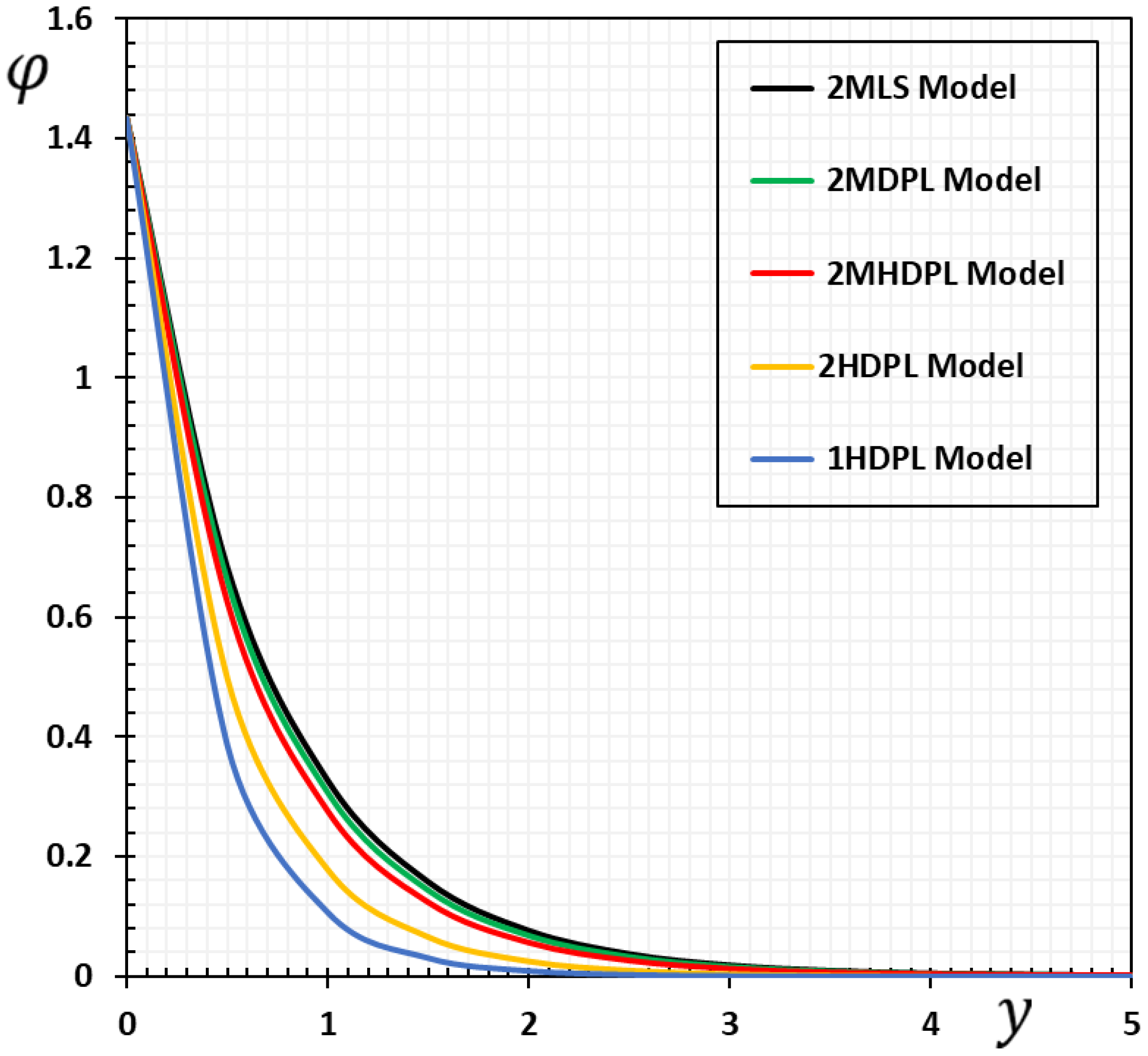
Figure 2 displays the effect of micropolarity, the higher orders of time derivatives $m$ and $n$, and the discrepancy coefficient $a_1$ on the temperature $\theta$ profile versus $y$. In the direction of growth of the vertical distance y and in the direction of wave propagation, the dynamic temperature $\theta$ gradually decreases. It is detected from the figure that, in different theories, the temperature $\theta$ rises rapidly to its maximum value, which is called the “peak temperature” due to the presence of decreasing thermal load. Then, in a specific area, the capacity of heat gradually decreases until it fades. The figure also confirms that in the absence of micropolarity, the temperature values are much greater than in the case of its presence. As a result, the role of micropolarity in reducing heat wave propagation emerges.

By examining the figure and comparing the curves of the theory 2MHDPL, which includes higher orders of partial derivatives, and the theory of 2MDPL, it is clear that the presence of higher derivatives $m$ and $n$ leads to a limitation of heat spread within the medium. Another important observation that can be extracted from the figure is the role of the two-temperature parameter $a_1$ in changing the temperature distribution. By comparison, it appears that the temperature curve in the case of the 2HDPL model is much less than that of the curves of the 1HDPL theory. Micropolar thermoelasticity theory will be particularly beneficial in studying materials made up of bar-like molecules with micro-rotational effects and the ability to sustain body and surface couples. From the results obtained and as mentioned in [33,34], when analyzing geophysical difficulties, the micropolar elastic model is thought to be more realistic than the traditional elastic model.

As shown in Figure 3, in all cases where the conductive temperature $\phi$ begins at a constant value at the free surface of the medium, in full accordance with the thermal boundary conditions. For the generalized theory, the conductive temperature starts at its highest point at the origin (attributed to the diffusion of the thermal boundary) and gradually declines until it attains zero in the direction of the heat wave. When compared with the data for all two-temperature models, the conductive temperature $\phi$ deals with smaller values in the case of the 1HDP model when the discrepancy coefficient $a_1$ is omitted. This also shows the discrepancy in the results in the presence and absence of micropolarity. Furthermore, it is clear that higher-order derivatives $m$ and $n$ play an important role in reducing the thermal conductivity distribution. The behavior of micropolar materials depends on the material parameters, phase delay and micro-rotation, and the parameters of the higher time derivatives [14,29,35].

Figure 4 and Figure 5 exhibit the area variant in normal and transverse displacements $u$ and $v$ in the framework of different micropolar thermoelastic models. We notice that there is a large difference in the distribution of displacements in the presence and absence of a non-dimensional two-temperature parameter $a_1$. As shown in Figure 4 and Figure 5, the temperature parameter $a_1$ as well as the higher orders of the partial derivatives of time $m$ and $n,$ have a major influence on all displacements $u$ and $v$. The distribution of the displacements has the same pattern in all three cases that include the micropolar effect (2MLS, 2MDPL, and 2MHDPL) and differs significantly from the two cases in which the micropolar effect disappears (2HDPL, and 1HDPL).

The fluctuations in the vertical and shear stresses ${\sigma }_{xx}$, ${\sigma }_{yy}$ and ${\sigma }_{yx}$ are illustrated in Figure 6, Figure 7 and Figure 8 under the influence of the discrepancy coefficient $a_1$ and higher orders $m$ and $n$, in addition to the micropolar. From the figures, it is clear that the discrepancy coefficient $a_1$ has a considerable impact on all fields. We can also see that the effect of two temperature coefficient $a_1$ and higher orders $m$ and $n$ continues to reduce the levels of normal stresses and shear stresses. Depending on the value of the temperature difference as well as higher orders, the waves approach a steady state. In Figure 6, in the presence of the micropolar effect, the behavior of the contrast in the normal stress ${\sigma }_{xx}$ is observed to be similar over the entire scale, with differences in the degree of contrast. The figure also shows a reflection of the curves in the presence and absence of the micropolar, which highlights the prominent effect of the presence of the micropolar on the distribution of vertical stress ${\sigma }_{xx}$. Alharbi et al. [36] investigated the influence of mechanical strip stress on a mathematical model for a magneto-thermoelastic micropolar medium. They also demonstrated how the micropolar material constants influence stress factors.

It can be seen from Figure 7 and Figure 8 that the absolute value of the tangential stress ${\sigma }_{yy}$ in the case of micropolar theories (2MLS, 2MDPL, and 2MHDPL) is very small compared to the absolute values in the absence of micropolar (2HDPL, and 1HDPL) and vice versa in the case of shear stress ${\sigma }_{yx}$. From Figure 7 and Figure 8, it can be observed that the tangential thermal stress ${\sigma }_{yy}$ and the shear stress ${\sigma }_{yx}$ in the case of different theories fulfill the mechanical boundary conditions imposed on the problem at the free surface of the medium.

It can be seen from Figure 7 and Figure 8 that the absolute value of the tangential stress ${\sigma }_{yy}$ in the case of micropolar theories (2MLS, 2MDPL and 2MHDPL) is very small compared to the absolute values in the absence of micropolar (2HDPL and 1HDPL) and vice versa in the case of shear stress ${\sigma }_{yx}$. From Figure 7 and Figure 8 it can be observed that the tangential thermal stress ${\sigma }_{yy}$ and shear stress ${\sigma }_{yx}$, in the case of different theories, fulfill the mechanical boundary conditions imposed on the problem at the free surface of the medium. Because of the anisotropy and micropolarity, the values of the normal displacement, normal force stress and temperature distribution are significantly variable near the point of application of the heat source. This phenomenon is consistent with previous results, as in [56].

Figure 9 and Figure 10 show the variance of micro-rotation $\omega$ and tangential couple stresses $m_{yz}$ in the framework of the three theories that include the micropolar effect (2MLS, 2MDPL and 2MHDPL), and the two theories in which the micropolar effect is neglected (2HDPL and 1HDPL). A large difference in the values was observed due to the presence of the non-dimensional discrepancy coefficient $a_1$ as well as the higher orders of the partial derivatives $m$ and $n$.

8. Conclusions

In this article, a new heat transfer model with two temperatures is presented in the field of generalized micropolar thermoelasticity. When we distinguish the concept of two temperatures, the first (dynamic temperature) comes from the mechanical process and the second comes from the thermal process (conductive temperature). In addition to the above, the heat conduction equation includes higher orders for the partial derivatives of time. From the proposed model, many previous models can be obtained as special cases, whether in the presence or absence of the micropolar effects, as long as the discrepancy coefficient is neglected. The suggested thermoelastic model was used to examine the behavior of thermal stresses, temperatures, displacements, and micro-rotation in an isotropic, homogeneous, micropolar, thermoelastic half-space by means of normal mode analysis. Calculations and discussions showed the following conclusions:

• The results indicate that the discrepancy coefficient has a substantial influence on the thermoelastic distributions within the medium, but the effect on the displacements and thermal stress disturbances is very clear;
• There is a large discrepancy in the results between the cases of theories that include two-temperature and those that include one-temperature. The coefficient of two-temperature works to reduce thermal and mechanical waves. Thus, the study of elastic bodies in the case of two-temperature theories is more realistic than the generalized thermoelastic theory at one temperature. Thus, the so-called conductive heat wave must be separated from the so-called thermodynamic heat wave;
• Higher orders for partial derivatives play a critical role in all distributions of the investigated domain variables. Thermal and mechanical waves are reduced by using higher orders for partial derivatives. Thus, the extended theory with phase lag times and higher order derivatives may be a better option for describing thermoelasticity than the previous generalized theories as well as the traditional ones;
• Micropolarity has a substantial impact on all of the domains covered. Except for tangential stress and thermodynamical temperature, micropolarity has a diminishing influence on the magnitudes of all thermo-physical fields investigated.

Finally, when examining the real behavior of some properties of materials in conjunction with the appropriate geometry of the presented model, the proposed problem takes on a whole new meaning. For example, within the earth, precious materials such as oil and liquid-like elements are found in unrefined form, while the rocks and minerals present may be granular in nature. The fields of geomechanics, seismic engineering, soil dynamics, and other fields are also considered to have practical applications for the specialization of thermal elasticity and waves.