A Safe and Efficient Lane Change Decision-Making Strategy of Autonomous Driving Based on Deep Reinforcement Learning

Abstract

As an indispensable branch of machine learning (ML), reinforcement learning (RL) plays a prominent role in the decision-making process of autonomous driving (AD), which enables autonomous vehicles (AVs) to learn an optimal driving strategy through continuous interaction with the environment. This paper proposes a deep reinforcement learning (DRL)-based motion planning strategy for AD tasks in the highway scenarios where an AV merges into two-lane road traffic flow and realizes the lane changing (LC) maneuvers. We integrate the DRL model into the AD system relying on the end-to-end learning method. An improved DRL algorithm based on deep deterministic policy gradient (DDPG) is developed with well-defined reward functions. In particular, safety rules (SR), safety prediction (SP) module and trauma memory (TM) as well as the dynamic potential-based reward shaping (DPBRS) function are adopted to further enhance safety and accelerate learning of the LC behavior. For validation, the proposed DSSTD algorithm is trained and tested on the dual-computer co-simulation platform. The comparative experimental results show that our proposal outperforms other benchmark algorithms in both driving safety and efficiency.

1. Introduction

In a report by the WHO, about 1.35 million people worldwide die in road traffic accidents every year, which is equivalent to one traffic accident death every 24 s, and about 20 million to 50 million people suffer non-fatal injuries [1]. Statistics have also shown that almost 94% of fatal traffic accidents are caused by driver errors. Autonomous vehicles (AVs), as promising solutions to road traffic challenges, can not only help reduce accidents, but also significantly relieve traffic congestion [2]. For instance, if 90% of cars on American roads become driverless, the number of car accidents will fall from six million to 1.3 million [3]. The major challenge for the decision-making of autonomous driving (AD) is how to ensure safer and more efficient driving behavior according to the characteristics of surrounding dynamic objects.

The earliest autonomous vehicle projects can be traced back to the 1980s which were presented by Carnegie Mellon University and the University of Bundeswehr Munich [4]. After that, the opening of the DARPA grand challenge has been an effective catalyst for further prompting the development of automated driving [5]. In these competitions, manually tuned methods were successfully applied to AVs who participated [6,7]. Since the release of a taxonomy for AD by the SAE in 2014, car and software companies have actively developed their own advanced driver assistance systems such as adaptive cruise control (ACC) to exert efforts toward full automation drive. As mentioned, in the early stage of AD, rule-based methods were widely adopted to elaborate a driving strategy based on prior human knowledge and mathematical models [8]. However, the deficiencies within those tactics are also noteworthy: (1) in a highly interactive and complex environment, the modeling itself is very difficult; (2) when the environment has changed or is unknown, the model needs to be redesigned and lacks generalization ability. The lack of the ability to interact with the changing road environment and traffic participants gives rise to the advancement in the application of machine learning (ML) for the AD decision-making problem.

Deep learning (DL) methods, with little dependency of the manual tuning facility, can learn the desired behavior through training, and thus are well suited for the vehicle control problem in a dynamic environment [9]. The key drawback of these methods lies in the fact that there is a lack of adequate traceability and interpretation for the decision execution process. With the exception of the traditional modular method, the driving strategy can also be learned end-to-end, directly mapping observations to actions, with the aid of reinforcement learning (RL) [10]. Through trial and error, RL aims to learn the optimal behavior in the corresponding observation by interaction with the environment, though with very limited availability to low-dimensional state–action spaces. Recently, to deal with high-dimensional space problems, deep reinforcement learning (DRL) provides a satisfying solution by further exploiting the characteristics of DL. In implementing DRL to AD tasks associated with different scenarios, the design of appropriate reward function and the incorporation of safety rule as well as training efficiency are still open issues for further study [11].

Being widely adopted in the DRL algorithm architecture, the actor–critic (AC) method utilizes single-step updating of the value function, thus can achieve faster update speed and higher learning efficiency. Specifically, it has been proven to be efficient in solving decision-making problems in AD systems. However, there still remain some open issues to tackle. Firstly, how to integrate the DRL algorithm model into the AD system and make it work with other modules to improve the overall performance becomes a major challenge. Some researchers have attempted to integrate DRL model into motion planning or behavior planning modules [12,13]. However, as the number of learned behavior models increases, the training costs and demand for driving data will accordingly be increased, and simultaneously, the overall convergence speed of the learning model will be decreased. To this end, this paper adopted the AC method and integrated the DRL model into the low-level control module of the AD system, thus realizing end-to-end decision-making architecture, which optimizes the actions directly to the low-level actuator based on the perception information.

Second, safety is the primary consideration in accomplishing AD tasks [14,15]. Therefore, the design of the safety-related reward in the MDP model is indispensable to ensure the safety of the agent behavior. However, the low sampling rate and the deviation existing in the reward function design will significantly threaten the driving safety of an AV. Some efforts have been made in the agent training process to increase the probability of traversing dangerous events. For example, the dual experience pool replay strategy has been proved to be successful in an automated braking system design [16]. It also becomes natural to incorporate some hard constraints for a safer exploration process (i.e., directly on the actions before interaction with the environment) [17]. Even so, it could place excessive constraints on the vehicle’s driving efficiency. To compensate for this shortage, a prediction model was adopted to predict and reward the future multi-step states. According to the above analysis, we will not only introduce a dual experience pool replay method during training process, but also utilize an explicit safety checker combined with a prediction learner for a safe exploration process. It is believed that with the aid of such methods, safer driving behaviors can be guaranteed when facing unexpected imminent events for lane change tasks.

Finally, in the real environment, with the demand for continuous control of the AV, a large state–action space is required, and the number of optimization iterations for the agent’s learning will increase exponentially. To improve the learning efficiency, knowledge-based methods [18,19] are utilized. However, when the driving environment is highly uncertain, it is difficult to manually evaluate the optimal trajectory or strategy. Besides, humans may not have the relevant knowledge and skills themselves. Consequently, we implemented the reward shaping method, which can introduce additional reward signals to supplement rewards from the environment. This will enable us to ameliorate the sparsity and uninformativeness of rewards [20], thus greatly improving the efficiencies of training.

In this article, the improved DRL algorithm is proposed to manipulate the continuous actions of the AV for LC requests in a lane-decreasing highway environment. Our proposal is simulated and tested on a dual-computer co-simulation platform to validate its driving safety, efficiency, and comfort performance. The main contributions of this paper are in the following two aspects:

(1)

For AD tasks such as lane-changing in highway scenarios, the DRL model is integrated to optimize the continuous actions into the low-level vehicle control module, and a dual-computer co-simulation platform is built for verification.

(2)

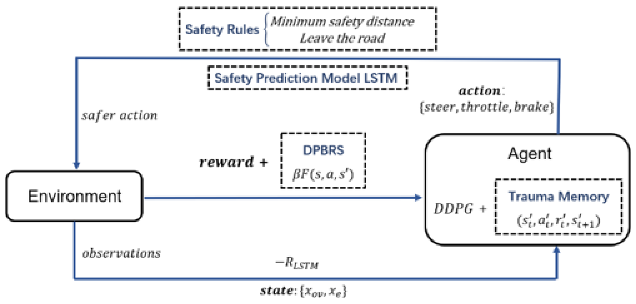
The Safety Rules module and the Safety Prediction module are both deployed explicitly and implicitly to impose some constraints on the output actions of the AV to enhance driving safety. During the agent training process, the trauma memory method is adopted to learn safer driving behavior when encountering emergencies in highway scenarios. Moreover, dynamic potential-based reward shaping is also implemented to improve the learning efficiency of the agent.

The remainder of this paper is organized as follows. A comprehensive literature review on the implementation of DRL method for AD tasks is presented in Section 2. Section 3 describes the DRL and the benchmark algorithm. The LC task and the MDP model in highway scenarios are described in Section 4. In Section 5, the DRL-based LC decision-making methodology is proposed. The simulation setup and results are discussed in Section 6, followed by our conclusions in Section 7.

2. Related Work

As one of the classic AC methods in the DRL algorithm, the deep deterministic strategy gradient (DDPG) [21] can use the function approximation based on deep neural network to learn continuous actions. This provides us with an effective way to solve the continuous action space problem in AD [22,23]. In addition, for scenarios with high environmental complexity and the requirements for large state–action space, the integration of the DRL model into the control module is regarded as a more feasible solution. Bojarski et al. [24] trained a nine-layer CNN by supervised learning to establish the steering policy and proposed an end-to-end AD control framework. However, their model could only be adapted for the lane keeping task. Tang et al. [25] utilized environmental information such as environment rasterization coding as the input to learn the driving behavior of the low-level control module through proximal policy optimization (PPO). In their work, the DRL model was integrated into the action control module in AD. Particularly, DDPG was utilized to evaluate continuous controls so that the continuous behavior decision was accessible to the low-level controller.

To improve driving safety, probability-directed exploration is an effective research direction. In [26], the Bayesian belief network-based approach was utilized to estimate the collision probability during driving, and safer actions were selected based on the evaluated safety strategy. Ref. [27] combined a model-checker with a RL policy to determine efficient policies with probabilistic safety guarantees. On the other hand, a considerable amount of research has focused on risk-directed exploration. Ref. [28] proposed the parallel constrained policy optimization algorithm (PCPO) to develop the expected risk function with safety constraints for relatively simple AD tasks. Similarly, ref. [29] proposed a risk-aware method to enable DQN to learn driving behaviors with lower risk coefficients, especially in high-risk environments. However, the above-mentioned methods all have challenges of utilizing learning-based methods to ensure functional safety. Therefore, it is necessary to request a low-level safety checker explicitly on the agent’s actions for driving safety. At the same time, there has been extensive research on the implementation of prediction model methods to RL. The authors in [30] proposed a prediction model based on dynamic graphs to achieve stable and effective long-term predictions of traffic flow. In [31], the original image data were utilized and partially processed as the input of the neural network to have a good predictive ability of the surrounding environment information during the navigation task. In contrast, we exploit the long short-term memory (LSTM) based prediction model to make up for the shortage of hard constraints on the actions. Furthermore, it is also necessary to enhance the driving safety by increasing the traversing probability of disastrous events. Ref. [32] proposed an automated braking system through training and testing with natural datasets so that the speed could be smoothly controlled in response to emergencies. When such emergency braking failed, [33] turned to detecting the pedestrians’ intentions in advance and performed evasive actions. Meanwhile, [34] proposed a threat-assessment algorithm suitable for multiple vehicle types, and the rear-end collisions were greatly reduced through the appropriate regulation of braking time. Inspired by [17,35], we adopted the trauma memory (TM) method to solve our highway LC decision problem to construct a separate experience pool for storing memories of dangerous emergencies, aiming to increase the traversal probability of such events in the agent training process.

The major influential factor for learning efficiency is highly related to the reward design. As a basic approach for enriching rewards [36], reward shaping has been extensively studied. Ref. [37] proved that the learning strategy of belief reward shaping (BRS) based on the Bayesian method was consistent with the optimal strategy of the original MDP. Demir et al. [38] utilized the difference in hidden states between landmarks to build the abstract model and solve the POMDP problems by reward shaping. In [39], the sub-goals obtained through the expert trajectory were utilized for reward shaping. To the above analysis, we introduce the DPBRS to shape the reward function to improve the learning efficiency of the agent.

3. Background

In this section, we introduce the basics of DRL and the essential framework of the benchmark DDPG algorithm. The main abbreviations are listed in

Table 1. Main abbreviations.

Abbreviation	Explanation
ML	Machine Learning
RL	Reinforcement Learning
DL	Deep Learning
AD	Autonomous Driving
AV	Autonomous Vehicle
AC	Actor–Critic
LC	Lane Change
DRL	Deep Reinforcement Learning
DDPG	Deep Deterministic Policy Gradient
DPBRS	Dynamic Potential-Based Reward Shaping
ETA	Estimated Time of Arrival
SORL	Survival-Oriented Reinforcement Learning
SR	Safety Rules
SP	Safety Prediction
LSTM	Long Short-Term Memory
TM	Trauma Memory
MDP	Markov Decision Process
DQN	Deep Q-network
IDM	Intelligent Driver Model
MOBIL	Minimizing Overall Braking Induced by Lane changes
TTC	Time-To-Collision
PPO	Proximal Policy Optimization
DST	DDPG + SR + TM
DSTD	DDPG + SR + TM + DPBRS
DSSTD	DDPG + SR + SP + TM + DPBRS

.

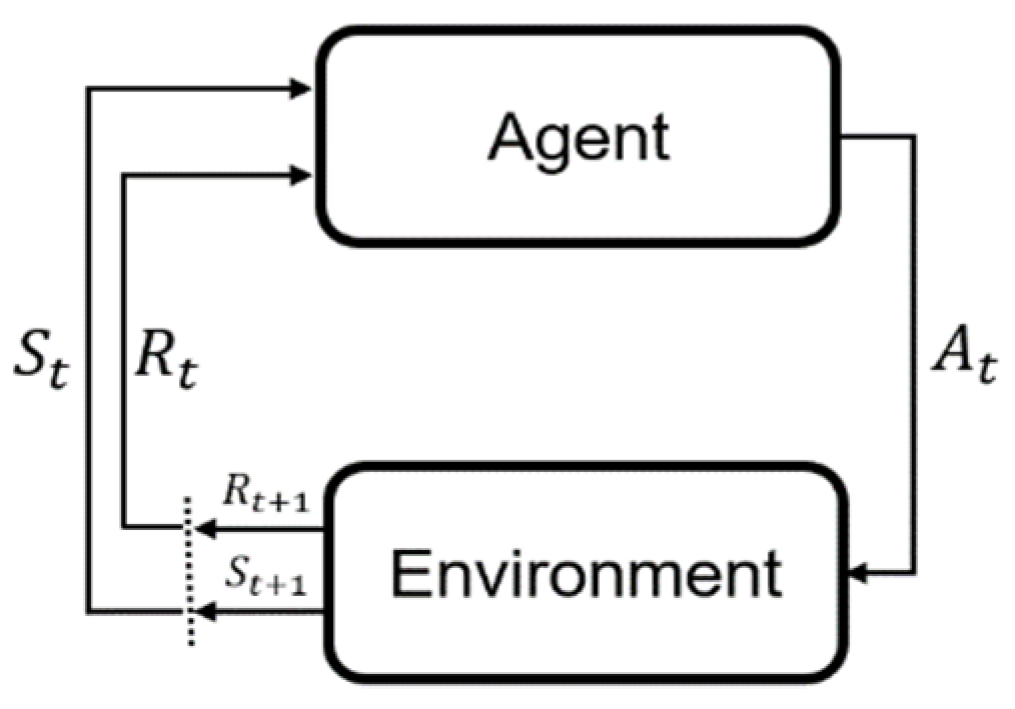
3.1. Deep Reinforcement Learning

The Markov decision process (MDP) is a mathematical model of sequential decision. In the simulation of MDP, the agent perceives the current state of the system and implements actions on the environment according to the strategy, thereby changing the state of the environment and obtaining rewards. The accumulation of rewards over time is called return. RL is used to describe and solve problems in which agents learn strategies to maximize the return or achieve specific goals in the process of interacting with the environment. The two are similar in terms of maximizing the cumulative reward of the agent, so RL often uses MDP as the standard model. As shown in Figure 1, almost all RL problems can be transformed into MDP, which basically consists of a four-tuple $\{S,A,R,P\}$: state S, action A, reward R, and state transition probability P. The transition function P contains three variables, which represents the dynamic transition process of the environment denoted by $p(s^{\prime }|s,a)$. For any current state $s\in S$, the agent first chooses the action $a\in A$, and then generates the next state by $s^{\prime }=P(S^{\prime }=s|S=s,A=a)$. The reward value R under the current state–action pair $(s,a)$ is calculated by the reward function $r(s,a)$, that is, $r:S^{\prime }\times A\times S\to R$. The state–action pair $(s,a)$ is composed of the current state s of the agent and the corresponding action a taken. The agent will evaluate the pros and cons of behavioral strategies through the reward values corresponding to different state–action pairs. RL is the process of running an agent through a sequence of state–action pairs and modeling complex probability distributions of a large number of state–action pairs and their associated rewards.

The ultimate goal of the agent in RL is to obtain the optimal behavior strategy through continuing trial and error. In other words, we can maximize cumulative reward G_t, which can be expressed as: $(a|s)=P(A_t=a|S_{t-1}=s)$, through continuing trial and error. In other words, we can maximize cumulative reward G_t, which can be expressed as:

$$\begin{array}{cc}\hfill G_t& =R_{t+1}+\gamma R_{t+2}+{\gamma }^2{R}_{t+3}+{\gamma }^3{R}_{t+4}+\dots +{\gamma }^{T-1}{R}_{t+T}\hfill \\ & ={\displaystyle \sum _{k=0}^{T-1}{\gamma }^k{R}_{t+k+1}}\hfill \end{array}$$

(1)

where t represents the current time and $\gamma \in [0,1]$ (usually set between 0.9 and 1) represents the discount factor that is used to measure the future reward value in the cumulative reward of the current time. T is the duration of the training trajectory. Moreover, the state value function $v_{\pi }(s)$ and state–action value function $Q_{\pi }(s,a)$, which are used to evaluate whether the strategy function is optimal, can be calculated by:

$$\begin{array}{c}{v}_{\pi }(s)=\mathbf{E}[G_t|S_t=s]\\ Q_{\pi }(s,a)=\mathbf{E}[G_t|S_t=s,A_t=a]\end{array}$$

(2)

From Equation (1), the above two value functions can be reformulated recursively by:

$$\begin{array}{c}{v}_{\pi }(s)={\displaystyle {\sum }_a\pi (s|a){\displaystyle {\sum }_{s^{\prime }}{P}_{s{s}^{\prime }}^a}}[G_{s{s}^{\prime }}^a+\gamma v_{\pi }(s^{\prime })]\\ Q_{\pi }(s,a)={\displaystyle {\sum }_{s^{\prime }}{P}_{s{s}^{\prime }}^a}[G_{s{s}^{\prime }}^a+\gamma {\displaystyle {\sum }_{a^{\prime }}{Q}_{\pi }(s^{\prime },a^{\prime })}]\end{array}$$

(3)

The Bellman optimality equation can be synthesized by using the above two relations and the optimal strategy can then be expressed as:

$$v^{\ast }(s)=ma{x}_a{\displaystyle {\sum }_{s^{\prime }}{P}_{s{s}^{\prime }}^a}[G_{s{s}^{\prime }}^a+\gamma {\displaystyle {\sum }_{a^{\prime }}{Q}_{\pi }(s^{\prime },a^{\prime })}]$$

(4)

3.2. DDPG Algorithm

Recently, Q-learning based RL methods have been extensively adopted to deal with decision-making problems [40,41]. However, they are only applicable to discrete action space and cannot effectively handle high-dimensional conditions.

Unlike DQN, which deals with discrete, low-dimensional actions, DDPG combines AC and DQN [42] algorithms to treat continuous action space problems. This is due to the fact that the output is not the probability distribution of the action behavior, but the specific mechanism of the deterministic continuous action value. Here, we utilized DDPG as the benchmark for realizing smoother driving behavior. In general, it has four neural networks, in which the Actor and the Critic have the same network structure and both have target-net and eval-net. According to the current state–action pair $(s,a)$, the Critic network can yield the estimated $Q(s,a)$ value. The agent adjusts the prediction level of the Q function by observing the reward value caused by the state–action pair $(s,a)$ until it can accurately predict the optimal strategy the agent should take. The Actor target network can yield A′ from the next state S′, and the Critic target network can evaluate the A′ by the output $Q^{\prime }(s^{\prime },a^{\prime })$ value. The TD-error between the $Q$ and $Q^{\prime }$ values is ultimately minimized, and the gradient ascent approach is exploited to update the Actor network to evaluate the action that can maximize the $Q(s,a)$ value. The DDPG algorithm flowchart is illustrated in Figure 2.

The “soft” update method ensures that the target network of DDPG can be updated in each iteration. The parameter change of the target network is small, and the update is relatively stable. Updating the Critic target and Actor target networks can be represented by:

$$\begin{array}{l}{\theta }^{{\phi }^{\prime }}\leftarrow \tau {\theta }^{\phi }+(1-\tau ){\theta }^{{\phi }^{\prime }}\\ {\theta }^{{\mu }^{\prime }}\leftarrow \tau {\theta }^{\mu }+(1-\tau ){\theta }^{{\mu }^{\prime }}\end{array}$$

(5)

where τ is an update parameter and can be set as τ « 1. $\phi$ and $\mu$ represent the current critic network and the current actor network, respectively. ${\phi }^{\prime }$ and ${\mu }^{\prime }$ represent the target critic network and the target actor network, respectively. $\theta$ represents the updated parameter of the corresponding network. To increase the randomness of the action and improve the exploration ability, Ornstein–Uhlenbeck (OU) noise N is added to the output action of the Actor by:

$$\mu (s)=\pi (s|{\theta }^{\mu })+N$$

(6)

where $\pi$ is the policy adopted by the Actor network in the current state s. Through the optimization process, the parameters of the current Critic network are updated by using the gradient backpropagation of the neural network. The loss function to be minimized can be formulated in terms of mean square error (MSE) by:

$$y_i=R_i+\gamma Q^{\prime }({s^{\prime }}_i,{a^{\prime }}_i|{\theta }^{{\phi }^{\prime }})$$

(7)

$$L=\frac{1}{M}{\displaystyle {\sum }_i{(y_i-Q(s_i,a_i|{\theta }^{\phi }))}^2}$$

(8)

where $y_i$ is the target Q value of the current critic network. $R_i$ is the reward return value in the target Q value of the current critic network, where i represents the ith sample collected from the experience pool, and $\gamma$ is the attenuation factor, usually set 0.9. The loss L can be evaluated by MSE with the current Q value, where M is the total number of samples collected from the experience pool. Note that for the current network of Actors, we used a deterministic strategy. The Q value generated by the Critic is used to determine the output action. According to the policy gradient criteria, the loss gradient of the current actor network can be defined by:

$${\nabla }_{{\theta }^{\mu }}J=\frac{1}{M}{\displaystyle {\sum }_i{\nabla }_a\phi (s_i,a_i|{\theta }^{\phi }){\nabla }_{{\theta }^{\mu }}\mu (s_i|{\theta }^{\mu })}$$

(9)

where J is the loss function of the current actor network with ${\theta }^{\mu }$ as the parameter, and $\nabla$ represents the loss gradient update for ${\theta }^{\mu }$ in J.

4. Problem Formulation

In this section, we first depict the specific lane-changing task considered in this paper. Then, a MDP model is exploited to formulate this LC decision making problem in the highway scenarios.

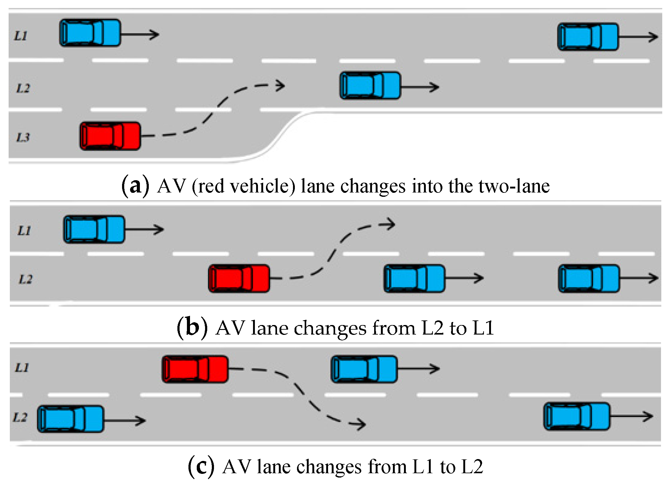
4.1. Lane-Changing Task

As shown in Figure 3, the LC behavior of the AV can be realized by a DDPG-based strategy. The driving strategy should ensure that the AV can adapt the trajectory characterized by the driving behavior of the surrounding vehicles while the intelligent driver model [43] (IDM) and minimizing overall braking induced by lane changes [44] (MOBIL) strategy can be employed to control the lateral and longitudinal motion of the surrounding vehicles. In this way, a training environment with high complexity will be close to real driving situations faced by human drivers. The final LC task to be solved is to avoid AV collisions with the surrounding vehicles and achieve high driving efficiency with smoothly executed maneuvers.

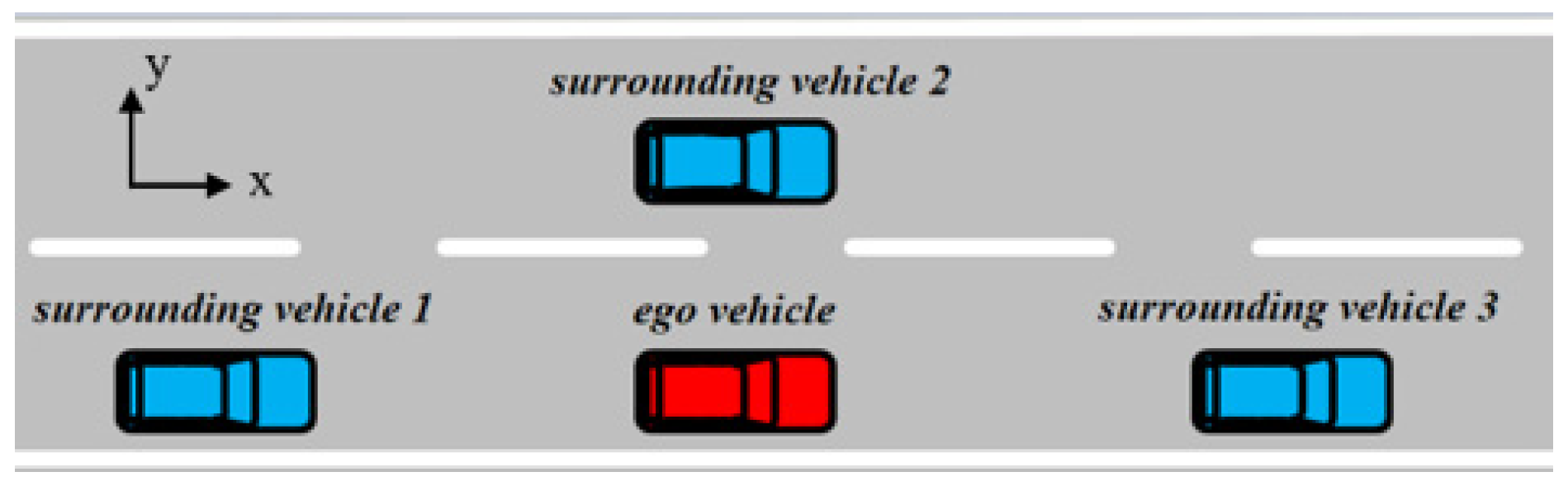
4.2. State and Action Space

We consider the state of four vehicles involved in the lane change decision and execution process as shown in Figure 4: (1) the ego vehicle; (2) the surrounding vehicles 1 and 3 in the same lane; and (3) the surrounding vehicle 2 in the target lane.

The state space $s_{set}$ of the RL model is an important basis for long-term returns evaluation and can directly affect the convergence of the algorithm. In this work, it is constructed by the state information of the target vehicle and surrounding vehicles, which can be expressed as:

$$\begin{array}{c}{s}_{set}=\{s_e,s_{ov}\}\\ s_e=\{x,y,v,a_e,{\theta }_e,\Delta d,l,t_{ttc},A_{steer},A_{throttle},A_{brake}\}\\ s_{ov}={\{v_i,\Delta v_i,\Delta x_i,\Delta y_i\}}_{i=1,2,3}\end{array}$$

(10)

where $s_e$ represents the driving state information of the target vehicle including position x, y, velocity v, acceleration $a_e$, compass heading angle ${\theta }_e$, lane centerline deviation $\Delta d$, the relative distance l between the AV and the leading vehicle in the same lane in the longitudinal direction. Time-To-Collision (TTC) is $t_{ttc}$ = $\Delta x$/$\Delta v$, where $\Delta x$ and $\Delta v$ represent the relative distance and relative speed, respectively, between the AV and the front vehicle in the same lane in the longitudinal direction (x-direction). $s_{ov}$ designates the state information of three surrounding vehicles including relative position information $\Delta x_i$, $\Delta y_i$ and velocity information $v_i$, $\Delta v_i$. i is the number of the surrounding vehicles, and $\Delta v_i$ represents the relative speed value between the AV and the all surrounding vehicles. $A_{steer}$, $A_{throttle}$, and $A_{brake}$ are the normalized values of steering wheel angle, throttle, and brake, respectively. It should be noted that all state quantities in the state space in the MDP are simply normalized, and the values are mapped between (0, 1), which is also to make the reward value easier to converge during subsequent agent training.

Based on the end-to-end low-level action control strategy, the action space of the RL model contains three ingredients, the steering wheel angle steer, the percentage of maximum throttle throttle, and brake pressure brake, which are specified as $A_{steer}\in (-20,20)$, $A_{throttle}\in (0,100)$, $A_{brake}\in (0,20).$ We utilized $A_{steer}$ to control the lateral motion of the AV, and $A_{throttle}$ and $A_{brake}$ to maneuver the longitudinal motion of the AV. The advantage of the end-to-end learning method lies in the fact that the training datasets can be either obtained from, or applied to the real world.

The lower-level controller receives the three action values from the output of the RL algorithm and converts them into appropriate wheel angles in conjunction with the 2D simple dynamics model to control the vehicle states.

4.3. Reward Function

The development of the reward function is another crucial part in the RL algorithm design. The externalization and numeralization of the task objective will determine whether the agent can learn the desired optimal LC driving strategy. Lane changing is a time sensitive task that needs to be completed as soon as possible once it is initiated. Taking into account various influential factors related to driving efficiency and safety, the construction of the reward function should consider the following aspects:

(1)

Efficiency-related reward $R_e$: This contributor aims to allow the AV to drive as fast as possible if permitted until the desired velocity is maintained. Simultaneously, if the vehicle’s departure from the lane centerline becomes larger, more penalties should be granted. For these reasons, the efficiency-related reward can be formulated by

$$R_e={\alpha }_1\cdot min(\frac{v-v_d}{v_d},0)-{\alpha }_2\cdot max(\frac{v-v_d}{v_d},0)-\frac{\Delta d^2}{3}$$

(11)

where $\alpha \in {\mathbf{R}}^{+}$ are the weighting parameters and v and $v_d$ represent the real velocity and the desired velocity of the AV, respectively.

(2)

Comfort-related reward $R_c$: This dedicator intends to enable the learning of smoother and more comfortable driving behavior by reducing the comfort deterioration due to excessive sudden changes in the vehicle state:

$$\begin{array}{l}{R}_c=-({\alpha }_3\cdot max(|{\dot{a}}_e|-{\dot{a}}_{cmax},0)+{\alpha }_4\cdot max(|a_e|-a_{cmax},0)\\ +{\alpha }_5\cdot max(|\Delta {\theta }_e|-10,0))\end{array}$$

(12)

where $a_e$ is the acceleration; $a_{cmax}$ is the maximum comfortable acceleration; ${\dot{a}}_e$ is the derivative of acceleration (also called Jerk [45]), ${\dot{a}}_e$ = $\Delta a_e$/$\Delta t$; and ${\dot{a}}_{cmax}$ is the maximum Jerk. Here, we let $a_{cmax}$ = 5 m/s² and $|{\dot{a}}_{cmax}|$ = 2 m/s³. The third term in $R_c$ limits the rate of change of the compass heading angle change $|\Delta {\theta }_e|$ to control the yaw motion caused by large angle changes in the driving direction.

(3)

Safety-related reward $R_s$: To ensure driving safety, the AV should learn to keep a safe distance from the leading vehicle in the same lane in the longitudinal direction (x-direction) to reduce collision. Thus, the safety-related reward can be adopted by

$$\begin{array}{l}{R}_s=-({\alpha }_6\cdot max(\frac{2.5-t_{ttc}}{2.5},0)+{\alpha }_7\cdot min(\frac{l-l_d}{l},0)\\ +{\alpha }_8\cdot max(\frac{l-l_d}{l},0))\end{array}$$

(13)

It can be shown that $t_{ttc}$ and reward have a negative correlation. Since the $t_{ttc}$ value is not expected to be small, it is believed that when $t_{ttc}$ < 2.5 [46], a small $t_{ttc}$ yields a small reward. The latter two terms in Equation (13) rely on the difference between the relative distance l between the AV and the leading vehicle in the same lane in the longitudinal direction and the desired relative distance $l_d$ to achieve safe distance control.

(4)

Terminal-related reward $R_t$: When the AV meets the required conditions during the simulation, the whole process will be terminated. We divid the termination requirements into two parts: positive reward value and negative reward value (for penalty use), which can be represented by

$$R_t=\{\begin{array}{cc}-{\alpha }_9\cdot P_1& ifcollisionoroffroad\\ {\alpha }_{10}\cdot P_2& ifcompletesthedesiredgoal\\ 0& otherwise\end{array}$$

(14)

where $P_1$, $P_2$ is set to have large positive values. If the AV collides or leaves the lane, a larger negative penalty will be utilized. Instead, whenever it successfully completes the expected LC task and drives to the desired target position, a larger positive reward is deployed.

Overall, the final reward function can be formulated by the summation of the weighted sum of the above sub-goals and the constant term c in the following way

$$R=w_1{R}_e+w_2{R}_c+w_3{R}_s+w_4{R}_t+c$$

(15)

where c motivates the vehicle to drive forward; $w_i$ represents the weight value of the four reward items, usually set between (0, 1), and the size of the weight value symbolizes the proportion of the corresponding reward item in the total reward formula, which needs to be manually set and adjusted.

5. Methodology

We first describe the algorithm architecture of the proposed LC strategy in this section. Then, we introduce methods to improve the driving safety from the external (SR + SP) and internal (TM) aspects of the agent. Finally, we describe the method (DPBRS) to improve the agent learning and driving efficiency.

5.1. Decision-Making Strategy Algorithm Architecture

The algorithm architecture of the proposed autonomous LC decision-making strategy is illustrated in Figure 5. Through the sensor data in Prescan/Simulink, the real-time states $x_{ov}$ and $x_e$ of all vehicles in the environment can be evaluated. The agent first initiates continuous actions (such as steer, throttle, and brake) at each time step, which will go through the inspection of the SR module. If driving safety is assured, these actions will be executed, or will be otherwise replaced with the prescribed safer actions. In addition, the SP model developed with LSTM will predict the future multi-step state vectors according to the current state action pair of the agent. By judging the dangerous situations (collision or offroad) of the future state vectors, a negative reward value is penalized in the reward function in the agent. The reward, as the result of the interaction of the environment, is then fed back to the agent after the implementation of DPBRS. The agent next combines the normalized states with the action and reward to establish a mini-batch of each time step, and employs the DDPG algorithm along with the TM method for data storage and training.

5.2. Safety Enhancement

5.2.1. Safety Rules (SR) + Safety Prediction (SP) Module

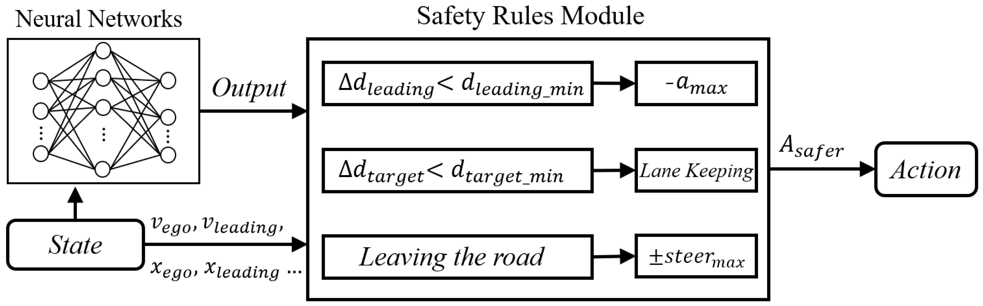
During the training process, the agent will learn to keep trying interactions with the environment. However, in real driving situations, leaving the lane and colliding are risky behaviors that must be avoided at all times. Even in training, it is necessary to prevent these from happening. Improving the driving safety of the agent from the perspective of improving the learning process cannot obtain sufficient trust. In order to ensure safer driving behavior, it is necessary to introduce SR related to hard constraints as a low-level safety layer. When the current state of the ego vehicle meets the constraints of the established safety layer, it will execute the constraint action in the SR module. Otherwise, it will directly execute the output action of the neural network. We design the following SR module [47,48] by considering two aspects of collision and offroad. The chart flow of the SR module is illustrated in Figure 6.

(1)

The minimum safe distance from the leading vehicle $d_{leading\_min}$: When the speed of the AV exceeds that of the leading vehicle driving in the same lane and the minimum safety distance between the two vehicles is breached, it is highly probable that a collision will occur if a certain deceleration maneuver is not performed. To avoid this, the minimum safe time interval $t_{min}$ can be introduced to satisfy:

$$t_{min}=inf\left\{t:t>\frac{2(v-v_{front})}{a_{dmax}}\right\}$$

(16)

where v and $v_{front}$ represent the speeds of the AV and the leading vehicle in the same lane, respectively, and $a_{dmax}$ implies the maximum deceleration of the AV. Correspondingly, the minimum safety distance $d_{leading\_min}$ should also satisfy:

$$d_{leading\_min}=(v-v_{front})\times t_{min}$$

(17)

$$\Delta d_{leading}=|x_{av}-x_{leading}|$$

(18)

where $x_{leading}$, $x_{av}$ represent the horizontal coordinates of the leading vehicle in the same lane and the AV, respectively. When the relative distance between the two vehicles $\Delta d_{leading}$ is less than the minimum safe distance $d_{leading\_min}$, the AV will attain the maximum deceleration $-a_{dmax}$. Otherwise, the AV will directly execute the throttle and brake pressure output by the neural network to accelerate and decelerate.

(2)

The minimum safe distance from the vehicle in the target lane $d_{target\_min}$: When the AV attempts to change lanes, it is essential to determine whether the relative distance between itself and the front vehicle or the behind vehicle in the target lane meets the minimum safe distance requirement. Similarly, the minimum safe time interval between the AV and the front and behind vehicles in the target lane are $t_{front\_min}$ and $t_{behind\_min}$, respectively:

$$t_{front\_min}=inf\left\{t:t>\frac{2(v-v_{target\_front})}{a_{dmax}}\right\}$$

(19)

$$t_{behind\_min}=inf\left\{t:t>\frac{2(v_{target\_behind}-v)}{a_{dmax}}\right\}$$

(20)

where $v_{target\_front}$, $v_{target\_behind}$ represent the speed of the front and behind vehicles in the target lane, respectively. Correspondingly, the minimum safe distance between the vehicle in the target lane and the AV $d_{target\_min}$ can be described as:

$$d_{target\_min}=min\left\{\begin{array}{l}(v-v_{target\_front})\times t_{front\_min},\\ (v_{target\_behind}-v)\times t_{behind\_min}\end{array}\right\}$$

(21)

$$\Delta d_{target}=min\{|x_{av}-x_{target\_front}|,|x_{av}-x_{target\_behind}|\}$$

(22)

where $x_{target\_front}$, $x_{target\_behind}$ represent the horizontal coordinates of the front and behind vehicles in the target lane, respectively. If the distance between the vehicle in the target lane and the AV $\Delta d_{target}$ is less than the minimum safety distance $d_{target\_min}$, the steering wheel angle is maintained for lane keeping. Otherwise, the AV will perform lane changing actions according to the steering wheel angle output by the neural network.

(3)

Avoid leaving the road: Besides collision, leaving the road is also a dangerous driving behavior in real traffic scenarios. When the AV is about to leave the road, the maximum reverse angle is exploited to keep it driving in the same lane at the same speed. Inherently, similar operations will be implemented when the AV is in the opposite lane. The corresponding formula is described as follows:

$$A_{steer\_safe}=\{\begin{array}{c}\min \left\{A_{steer}\right\}ifleavetheleftroadline\\ \max \left\{A_{steer}\right\}ifleavetherightroadline\end{array}$$

(23)

where $\min \left\{A_{steer}\right\}$, $\max \left\{A_{steer}\right\}$ represent the minimum and maximum steering wheel angles taken by the AV when it is about to leave the left and right road lanes, respectively. According to the description of the MDP model action space, $\min \left\{A_{steer}\right\}$ and $\max \left\{A_{steer}\right\}$ are equal to −20 degrees and 20 degrees.

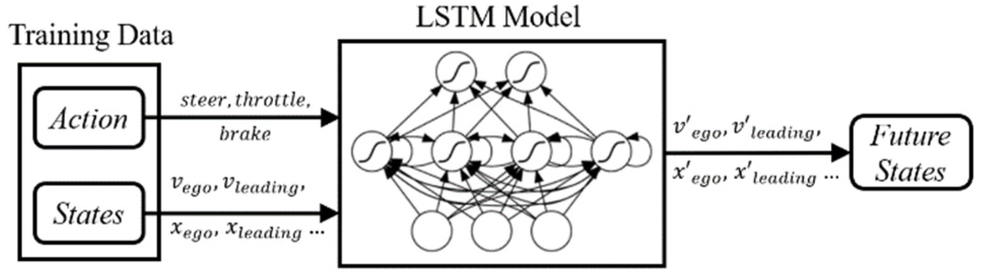
Due to the diversity of the driving behavior of the surrounding vehicles, the longitudinal restrictions by the SR module may not be enough to avoid the occurrence of the collision. On the other hand, it may over-constrain an AV’s transient motions [17]. In order to further improve safety and accelerate the learning process of the agent, we trained a LSTM network model to predict the future state of the AV. By judging the unsafe future states within the specified step size, the reward function of the RL model is granted by a corresponding penalty.

(1)

LSTM training: We utilize the state–action data of the RL model in 3000 rounds with the SR module in the test set as the training data of the LSTM prediction model in Figure 7. The state–action pairs in the last five simulation steps are employed as the input of the LSTM prediction model, and its output predicts the state vectors of the next five steps.

(2)

Judgment of the future states: If there are any dangerous states (collision or offroad) in the next five steps predicted by the LSTM prediction model, we store the state information of the next step in the TM and offer the reward function a larger penalty value of $-R_{LSTM}$

5.2.2. Trauma Memory (TM)

In the typical DDPG method, the replay memory experience pool will store the related sample $(s_t,a_t,r_t,s_{t+1})$ in each time step for training. Since vehicle collisions rarely occur with regard to SR, there are only a few collision-related state sets in the pool. As a result, these data will be adopted with a small probability during training. This can lead to insufficient learning opportunities in the training for collision avoidance. When faced with emergencies such as collisions, rule-based safety constraints are difficult in making reasonable and effective safety decisions. Therefore, to improve the safety, the learning efficiency, and the convergence speed, the TM [16] method was employed. When a collision occurs during training, the sample $({s^{\prime }}_t,{a^{\prime }}_t,{r^{\prime }}_t,{s^{\prime }}_{t+1})$ in the current time step is stored in a separate experience pool (named the “Trauma Memory Experience Pool”) to construct “dual experience pools” for sampling training. During this training, parts of samples are randomly selected from the replay memory pool while a fixed number are chosen from the TM related to imminent events. The corresponding loss function can be described as follows:

$$\begin{array}{cc}\hfill L& ={\displaystyle {\sum }_{i\in B_{replay}}{\delta }_i^2}+{\displaystyle {\sum }_{i\in B_{trauma}}{\delta }_i^2}\hfill \\ & =\frac{1}{M}({\displaystyle {\sum }_{i\in B_{replay}}{(y_i-Q(s_i,a_i|{\theta }^{\phi }))}^2+{\displaystyle {\sum }_{i\in B_{trauma}}{(y_i-Q(s_i,a_i|{\theta }^{\phi }))}^2}})\hfill \end{array}$$

(24)

where $B_{replay}$ and $B_{trauma}$ denote the original replay and the TM experience pool, respectively. ${\delta }_i$ denotes the time difference error; $M$ denotes the number of samples for batch gradient descent; and $y_i$ denotes the current target Q value. The collision-related sets are then randomly sampled from the dual pools of a fixed number (64 and 20, respectively) for training. This can continuously remind the agent of collision-related memories, especially for those dangerous emergencies in the experience pool that cannot be considered by rule-based safety constraints, and help it learn to reduce the possibility of such events with reasonable and effective actions. Eventually, through such accurate and effective evaluation of collision avoidance behaviors, driving efficiency and safety can be greatly strengthened.

5.3. Efficiency Improvement

When implementing the manually tuned reward functions, it has to face a sparsity problem of rewards, which inevitably results in slow convergence rates of the algorithm. More precisely, the agent needs to spend plenty of time frequently interacting with the environment for data sampling, and thus it becomes difficult to learn the optimal strategy from those limited number of samples. If the agent is simply rendered an additional positive reward after it approaches the final goal or accomplishes the sub-goal, it would find “flaws” and continue to wander around the sub-goal, consequently, unable to learn the optimal strategy.

To this end, by relying on the original reward function, we incorporat a potential-based reward [49] to formulate a new reward criterion by $R^{\prime }=R(s,a,s^{\prime })+\beta F(s,a,s^{\prime })$. More specifically, in addition to the environment reward signals, PBRS learns a reward-shaping function $F:S\times A\times S^{\prime }\to R$ to render auxiliary rewards, provided that the additional rewards contain external knowledge to guide the agent toward better action selections. Intuitively, the reward-shaping strategy will assign higher rewards to more beneficial state–action pairs, which can navigate the agent to the desired trajectories. The real-valued function F can be expressed in the form of potential difference as:

$$F(s,a,s^{\prime })=\gamma \varphi (s^{\prime })-\varphi (s)$$

(25)

where the potential function is defined as the mapping from the state to real-number by $\varphi :S\to \mathbf{R}$, and γ denotes the discount factor. This provides a sufficient and necessary condition for guaranteeing the consistency of the optimal strategies evaluated after ($H^{\prime }$ = (S, A, T, γ, R + F)) and before ($H$ = (S, A, T, γ, R)) reward shaping of the MDP model. $\varphi (s)$ is a potential function with state parameter s.

To allow for potential-based reward shaping for a dynamic potential function, we use time t as an additional parameter of the potential function $\varphi$ in Equation (25):

$$F(s,a,s^{\prime })=\gamma \varphi (s^{\prime },t^{\prime })-\varphi (s,t)$$

(26)

where t and $t^{\prime }$ represent the time the agent to the previous state s and to the current state $s^{\prime }$(i.e., t <$t^{\prime }$), respectively. Because the potential difference is calculated based on the state potential of the agent, the introduction of the time parameter t does not change the agent’s policy invariance or consistent Nash equilibria.

Moreover, the optimal Q functions Q* in the original and transformed MDP are related by the potential function $\varphi$:

$$Q_{H^{\prime }}^{*}(s,a)=Q_H^{*}(s,a)-\varphi (s,t)$$

(27)

which draws a connection between PBRS and advantage-based learning approaches. t is the current time.

In our case, a real potential value is assigned to each state of the vehicle in the y-direction. For instance, a positive reward was adopted when driving from a place with low potential energy to that with high potential energy; otherwise the negative reward with equal size is utilized. From the perspective of momentum potential energy in physics, this can also encourage the agent to always move to the target position with the highest potential energy, which helps to speed up the learning process.

The detailed process of the DSSTD algorithm is shown in Algorithm 1. Its input hyperparameters include the number of training episodes E, learning rate τ, etc., and the output is the LC control policy. In the initial phase of each round of agent training, the reinforcement learning algorithm randomizes parameters (such as ${\theta }^{\phi }$, ${\theta }^{\mu }$, etc.) in order to make the agent explore the environment state space more uniformly during the training process and reduce the correlation of the collected samples, which is conducive to learning the effective strategy distribution.

Algorithm 1. DSSTD Algorithm.

1: Initialize the weights ${\theta }^{\phi }$ and ${\theta }^{\mu }$ 2: Initialize the weights ${\theta }^{{\mu }^{\prime }}\leftarrow {\theta }^{\mu }$ and ${\theta }^{{\phi }^{\prime }}\leftarrow {\theta }^{\phi }$ 3: Initialize buffers:$B_{replay}$, $B_{trauma}$ 4: For episode = 1, E do 5: Initialize noise value N 6: Obtain state–action information 7: Receive initial state s1 8: For t = 1, T do 9: Select the output action $a_t$ 10: If the conditions are met     $a_t=a_{safer}$ 11: Execute action $a_t$ and obtain reward $r_t$ and next state $s_{t+1}$ 12: Store transitions $\left(s_t,a_t,r_t,s_{t+1}\right)$ and $\left({s^{\prime }}_t,{a^{\prime }}_t,{r^{\prime }}_t,{s^{\prime }}_{t+1}\right)$ in $B_{replay}$ and $B_{trauma}$ 13: Use LSTM to predict $s_{t+2}$, $s_{t+3}$, …, $s_{t+k}$ 14: If conditions are met    $r_t$ ← $-R_{LSTM}$ 15: Store transition $\left({s^{\prime }}_t,{a^{\prime }}_t,-R_{LSTM},{s^{\prime }}_{t+1}\right)$ in $B_{trauma}$ 16: Sample minibatchs $\left(s_t,a_t,r_t,s_{t+1}\right)$ and $\left({s^{\prime }}_t,{a^{\prime }}_t,{r^{\prime }}_t,{s^{\prime }}_{t+1}\right)$ from $B_{replay}$ and $B_{trauma}$ 17: Calculate loss function and Q value $Q(s_i,a_i|{\theta }^{\phi })$ 18: Update critic network 19: Update output strategy 20: Update AC networks 21: end for 22: end for 23: end while

6. Experimental Evaluation

In this section, the performance of the proposed LC decision-making strategy is verified on the dual-computer co-simulation platform by comparative simulations. We first present the simulation setup and the corresponding hyperparameter value settings. Then, we describe the initial setup of the scenario and the driving model of surrounding vehicles. Finally, we discuss the training result and test result in terms of driving safety, learning efficiency, and comfort.

6.1. Simulation Setup

Our proposed algorithm is implemented on a self-built dual-computer co-simulation platform. One host uses the Windows operating system to build the traffic training scenario in Prescan and constructed the vehicle low-level control model in MATLAB/Simulink. The other host employs the Ubuntu operating system to run the algorithm written in TensorFlow. Both two hosts adopt User Data Protocol (UDP) command and are connected via the Ethernet to establish communication, which can realize their data transmission. The diagram of the simulation platform is shown in Figure 8.

The state information in the Prescan traffic scenario is transmitted in real-time to the proposed algorithm in Ubuntu as the input value of the neural network. Then, the action value evaluated by the network is fed back to the vehicle low-level control module in MATLAB/Simulink. The corresponding actions are executed in the Prescan environment of host 1 based on the control demand transmitted from host 2. Thereby, the state of the next step of the AV is updated and cyclic transition can be realized. The single step time of the simulating episode is illustrated in Figure 9. At the beginning of the episode, there is a slightly longer feedback time, and the average single step time for the entire episode was 0.045 s.

Note that RL algorithms are adopted to only manipulate the driving behaviors for the AV. For the simulation setup, the maximum simulation time is set to 20 s, and the step size is set to 0.1 s. Fully considering the model complexity and the computation costs, the three hidden layers and their corresponding node numbers are selected as (64, 64, 32). The learning rates of the Actor and Critic are set to 0.001 and 0.002, respectively. The discount factor and soft updating rate are set to 0.99 and 0.001, respectively. For the implementation of the TM method, we set the mini-batch to have a 64 batch size from $B_{replay}$ and 20 batch size from $B_{trauma}$ during training. Due to the limitation of the computational cost, most hyperparameters are not adjusted systematically, but selected so that the satisfying training results could be met. The key hyperparameters set for the RL training process are listed in

Table 2. Parameter setting of the DRL process.

Parameters	Values
Discount factor	0.99
Actor network learning rate	0.001
Critic network learning rate	0.002
Size of hidden layers	(64, 64, 32)
Optimization algorithm type	Adam
Size of replay memory	1e5
Size of trauma memory	1e3
Batch size of replay memory	64
Batch size of trauma memory	20
Soft updating rate	0.001
Exploration	0.1

.

6.2. Initial Scenario and Surrounding Vehicles Driving Model

In the simulation scenario, the initial velocity of the AV (in red) is 10 m/s and the speeds of the surrounding vehicles (in blue) are randomly selected between 8 m/s and 12 m/s. The desired velocity of the AV is 23 m/s, and the velocity of the surrounding vehicles is limited to 20 m/s. The length and width of each vehicle are 4 m and 1.96 m, respectively. At the beginning, the AV drives in lane L3 with a length of 20 m, and the three surrounding vehicles drive in lanes L1 and L2, each with a length of 100 m.

As described previously, the surrounding vehicles use a driving model that combined IDM and MOBIL. IDM is used to evaluate the longitudinal acceleration for car-following and adaptive cruise controls of AVs, which can be written as:

$$\ddot{x}=a_{max}[1-{(\frac{\dot{x}}{{\dot{x}}_{sur}})}^{\lambda }-{(\frac{g_0+T_{gap}\dot{x}+\frac{\dot{x}\Delta \dot{x}}{2\sqrt{a_{max}b}}}{g})}^2]$$

(28)

where x is the displacement in the longitudinal direction of the vehicle; $\dot{x}$ and $\ddot{x}$ are the longitudinal velocity and acceleration of the vehicle, respectively; ${\dot{x}}_{sur}$ is the expected velocity of the surrounding vehicles; and g is the relative distance between AV and the leading vehicle in the same lane. Note that the model parameters λ, $g_0$, T_gap, a_max, and b are given within reason.

MOBIL is deployed to generate the LC command by evaluating the feasibility of the LC intention. It controls the LC behavior of the surrounding vehicles in the lateral direction, which can be realized by satisfying:

$$\begin{array}{c}{\overline{\ddot{x}}}_n\ge -b_{safe}\\ {\overline{\ddot{x}}}_c-{\ddot{x}}_c+\epsilon ({\overline{\ddot{x}}}_n-{\ddot{x}}_n+{\overline{\ddot{x}}}_o-{\ddot{x}}_o)>\Delta a_{th}\end{array}$$

(29)

where $\ddot{x}$ and $\overline{\ddot{x}}$ represent the current state and the transition state of the vehicle LC, respectively. The subscript c indicates the vehicle that will execute the LC action. The subscripts n, o indicate the following vehicles after and before the LC, respectively. The model parameters $\epsilon$ and $\Delta a_{th}$ were set within the reasonable range. The detailed parameter setting of IDM and MOBIL and the traffic scenario [45] are listed in

Table 3. Parameter setting of the scenario and the motion model of the surrounding vehicles.

Symbol	Parameters	Values
Length of three-lane	$l_1$	80 m
Length of two-lane	$l_2$	100 m
Length of converging-lane	$l_3$	20 m
Width of road	$w$	3.5 m
Length of vehicle	$l_v$	4 m
Width of vehicle	$w_v$	1.96 m
Initial velocity of the AV	$v_0$	10.0 m/s
Desired velocity of the AV	$v_d$	23.0 m/s
Initial velocity of surrounding vehicles	${v^{\prime }}_0$	[8~12] m/s
Limit velocity of surrounding vehicles	$v_{max}$	20.0 m/s
Actual acceleration of the AV	$\ddot{x}$	/
Actual velocity of the AV	$\dot{x}$	/
Desired velocity of surrounding vehicles	${\dot{x}}_{sur}$	15.0 m/s
Actual relative velocity	$\Delta \dot{x}$	/
Desired time gap	$T_{gap}$	1.0 s
Minimum relative distance	g0	10.0 m
Actual relative distance	$g$	/
Maximum acceleration	$a_{max}$	2.0 m/s2
Desired deceleration	b	(−)1.0 m/s2
Acceleration in transition state	$\overline{\ddot{x}}$	/
Safe deceleration limit	$b_{safe}$	1.0 m/s2
Acceleration argument	λ	4
the vehicle that will execute the LC	c	/
the following vehicles after the LC	n	/
the following vehicles before the LC	o	/
Politeness factor	$\epsilon$	0.001
Acceleration threshold	$\Delta a_{th}$	0.2 m/s2

.

6.3. Training Results

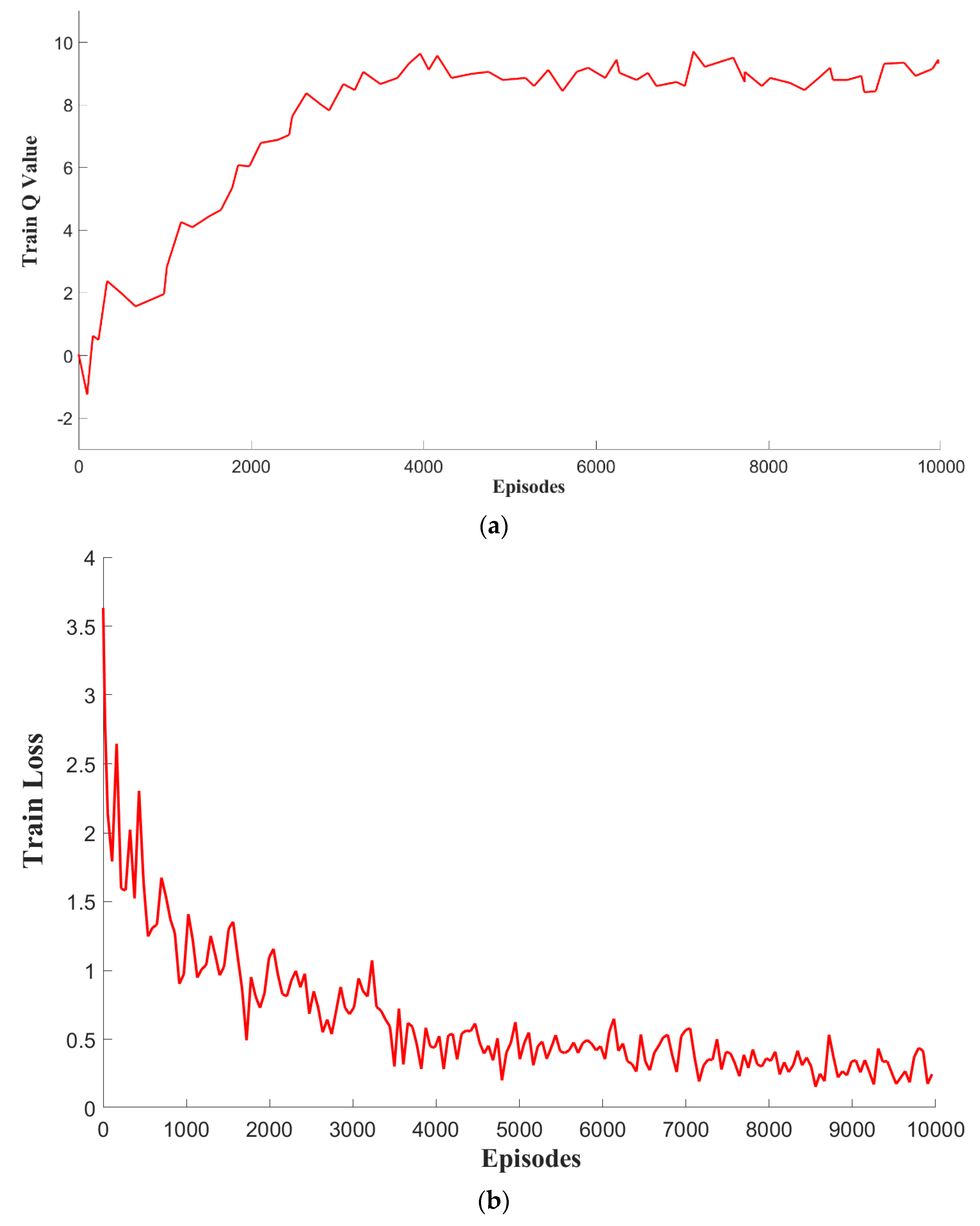
In our simulation, the agent is trained for 10,000 episodes.

In the training, we implemented and compare five algorithms including traditional DDPG, PPO, improved DDPG + SR + TM (DST), DDPG + SR + TM + DPBRS (DSTD), and DDPG + SR + SP + TM + DPBRS (DSSTD). We evaluated the stability of the proposed DSSTD model as shown in Figure 10. The average rewards obtained by the agent under different tactics are compared in Figure 11.

(1)

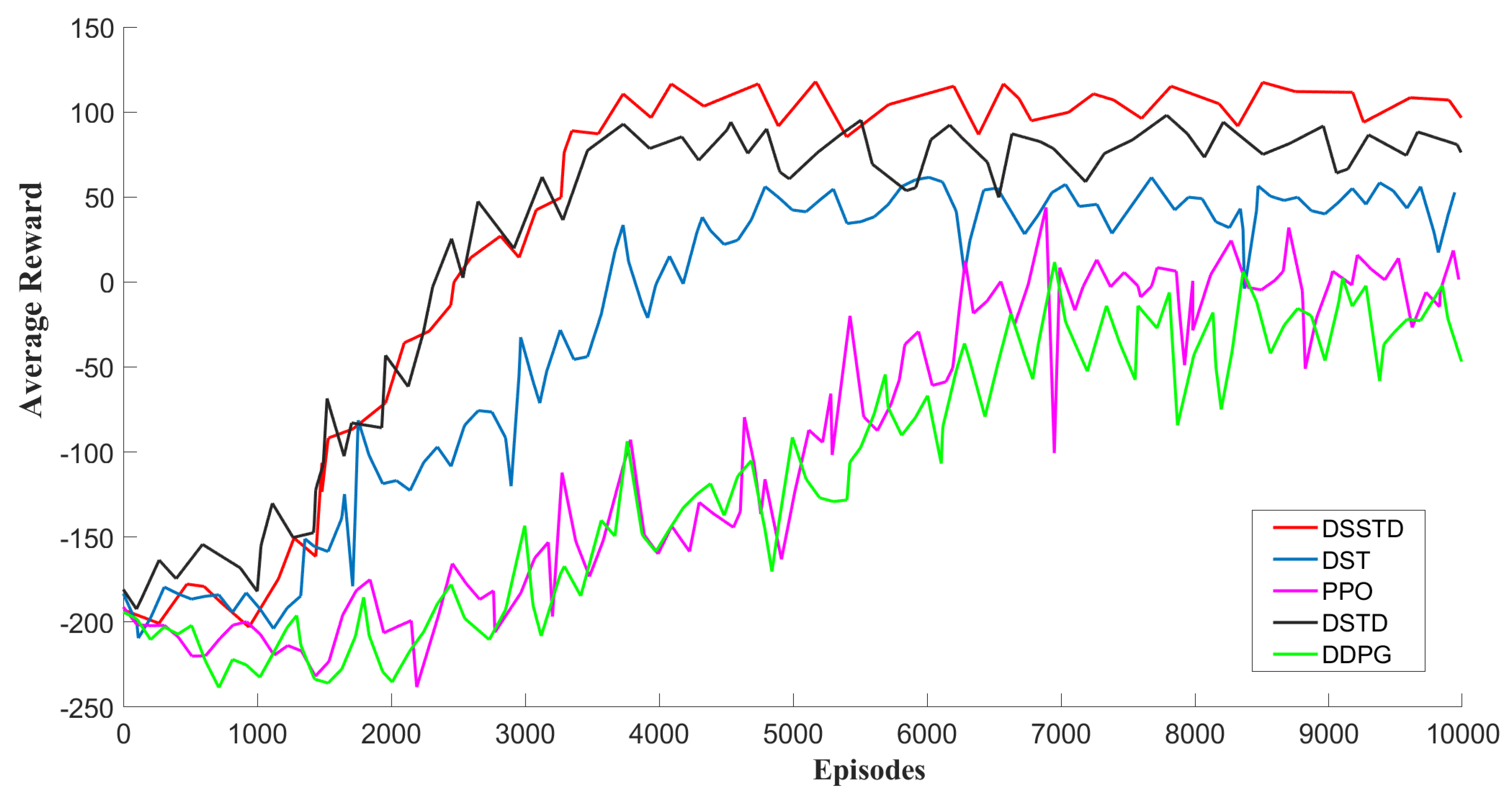
Evaluation of the proposed DRL model: To evaluate the stability of the proposed DRL model, we investigated the average Q value of the Actor network and the loss value of the Critic network in the DSSTD model during training. As shown in Figure 10a, the average Q value finally converged to the maximum value (9.86) around 4000 episodes. It could also be observed from Figure 10b that the loss values converged to the minimum value (0.33) around 4000 episodes. The result of the above converging phenomenon was well consistent with the stability performance of the DSSTD model, as shown in Figure 11. This demonstrated that our DSSTD model had good stability, and furthermore, the trained Actor network could output the action with the largest expected Q value and attain considerable cumulative returns. It is necessary to explain that the curve often experiences fluctuation in a smaller range after it converges, which could also be found on other studies [22].

(2)

Discussion on reward function: From Figure 11, it can be seen that as the training simulation progressed, the cumulative average rewards of the traditional DDPG or PPO algorithms gradually increased and eventually converged to be stable around 8000 episodes. If more training episodes are available, the traditional RL rewards tend to have fewer fluctuations after convergence, but may experience the divergence problem. Prior to being stabilized, they are prone to relatively large fluctuations around 7000 episodes and their convergence speeds were almost the same. The fact that a higher reward of PPO is granted indicates that its driving strategy outperformed traditional DDPG in safety and speed.

To prevent dangerous incidents as much as possible, SR and TM approaches were next implemented. Under the setting of fixed-length episodes, the rewards of DST converged faster than the traditional ones. Additionally, they stabilized around 5500 episodes and the corresponding values were also much higher.

Finally, with the DPBRS technique, the result showed that DSTD had a faster convergent rate than DST and eventually stabilized around 4000 episodes with less fluctuation. The resulting cumulative return was also higher than the other three. In addition, DSSTD also tended to converge around 4000 episodes and the average reward value (around 110) was greater than DSTD (around 90). Hence, it can be concluded that the DSSTD algorithm could have the most efficiency and the maximum long-term rewards in solving LC decision making problem.

6.4. Test Result

The training associated with the above five algorithms was performed for 500 rounds. The traditional DDPG and PPO used the MATLAB/Simulink RL toolbox for training and testing on the standalone computer simulation platform. DST and DSSTD were trained and tested on the proposed dual-computer co-simulation platform, in which the algorithm could be optimized flexibly and conveniently and the trained agent can probably be implemented for the actual vehicle experiment. The overall test results were compared in

Table 4. Comparison of different methods in the test.

Algorithm	DDPG	PPO	DST	DSTD	DSSTD
Lane change success rate (%)	87.6	90	98.8	98.4	100
Collision or off-road counts	59	48	6	8	0
Average speed (m/s)	22.3	22.62	22.48	23.12	23.03

.

Next, the analysis of the simulation results is presented in the following three respects: safety, driving efficiency, and comfort.

(1)

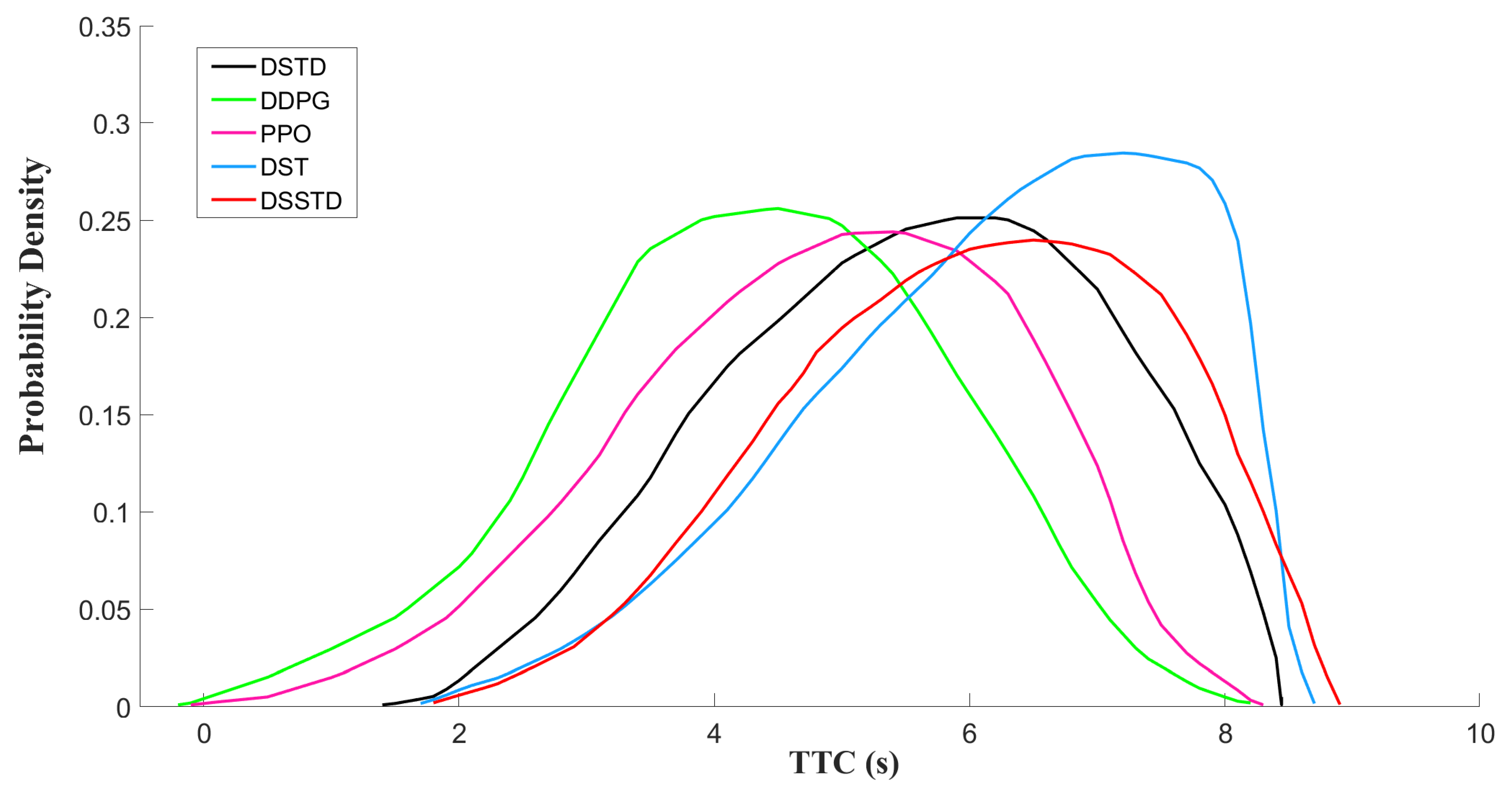
Safety: Here, four indicators including LC success rate, collision or off-road counts, the minimum distance to the leading vehicle, and the TTC, were utilized to evaluate the safety of AV during LC in the test round.

From Table 4, it can be shown that the traditional DDPG and PPO did not perform well in the test rounds. For example, DDPG achieved an 87.6% LC success rate, and had 59 collisions or offroad. In the other hand, the performance of PPO was slightly improved since the LC success rate and collision/offroad counts were 90% and 48 times, respectively. It is worth noting that most of the dangerous events such as collisions that occurred during the test round also took place during the lane-changing process. This indicates that the decision-making strategy that the agent has learned must not be optimal. Once encountering the situations with small vehicles gap and relative high speed, the agent may fail to make appropriate adjustment measures. In particular, excessive LC behavior or not slowing down could easily bring about a collision accident. Therefore, a LC success rate of about 90% was far from enough for real driving behavior. Comparing the traditional RL algorithm, the LC success rate of DST increased up to 98.8%. Collision or offroad counting dropped to six times. Obviously, DST with SR + TM achieved a great improvement in driving safety. Using DSTD, a 98.4% lane change success rate and eight collisions could be achieved. This result shows that DPBRS had no effect on driving safety. However, the DSSTD with SP model could guarantee 100% lane change success rate and 0 collisions. Compared with DSTD, the prediction method of the SP model greatly improved the driving safety and the lane change success rate during the test.

In the test round, the minimum relative distances of the five candidates were compared and are presented in

Table 5. Minimum relative distance to the leading vehicle.

Relative Distance (m)	DDPG	PPO	DST	DSTD	DSSTD
Surrounding vehicle 1	9.5	8.6	14.5	14.7	15.0
Surrounding vehicle 2	9.2	10.1	12.1	12.6	14.8
Surrounding vehicle 3	7.8	9.9	12.8	12.0	12.2

. The minimum relative distances specified to surrounding vehicle 3 by DDPG and surrounding vehicle 1 by PPO were 7.8 m and 8.6 m, respectively, which were far below the safety margin (10 m). In contrast, the minimum relative distance designated to surrounding vehicle 3 by DSTD and DSSTD were 12.0 m and 12.2 m, respectively, which were 0.8% and 1.6%, respectively, higher than 12.1 m regarding the distance specified to surrounding vehicle 2 by the DST. The proposed DSSTD algorithm allowed the AV to have sufficient space for optimal LC maneuvers.

TTC (Time-to-Collision) often serves as one of the indicators for safety evaluation during driving. Van et al. [47] analyzed the relationship between TTC information and collision probability to evaluate an empirical value of 1.5 s. When TTC is less than 1.5 s, the collision probability will be greatly increased. From observing the TTC distribution in Figure 12 (excluding the data with TTC greater than 8.5 s), it can be found that nearly 5.63% of the TTC distribution by DDPG were between 0 s and 1.5 s, which was larger than the result of PPO 4.48%. In contrast, the minimum values of TTC by DST and DSSTD were both around 1.8 s, which was much bigger than the red line of 1.5 s. Therefore, our proposed DST and DSSTD performed better in reducing the overall collision risk when faced with an emergency than the traditional DRL algorithms.

(2)

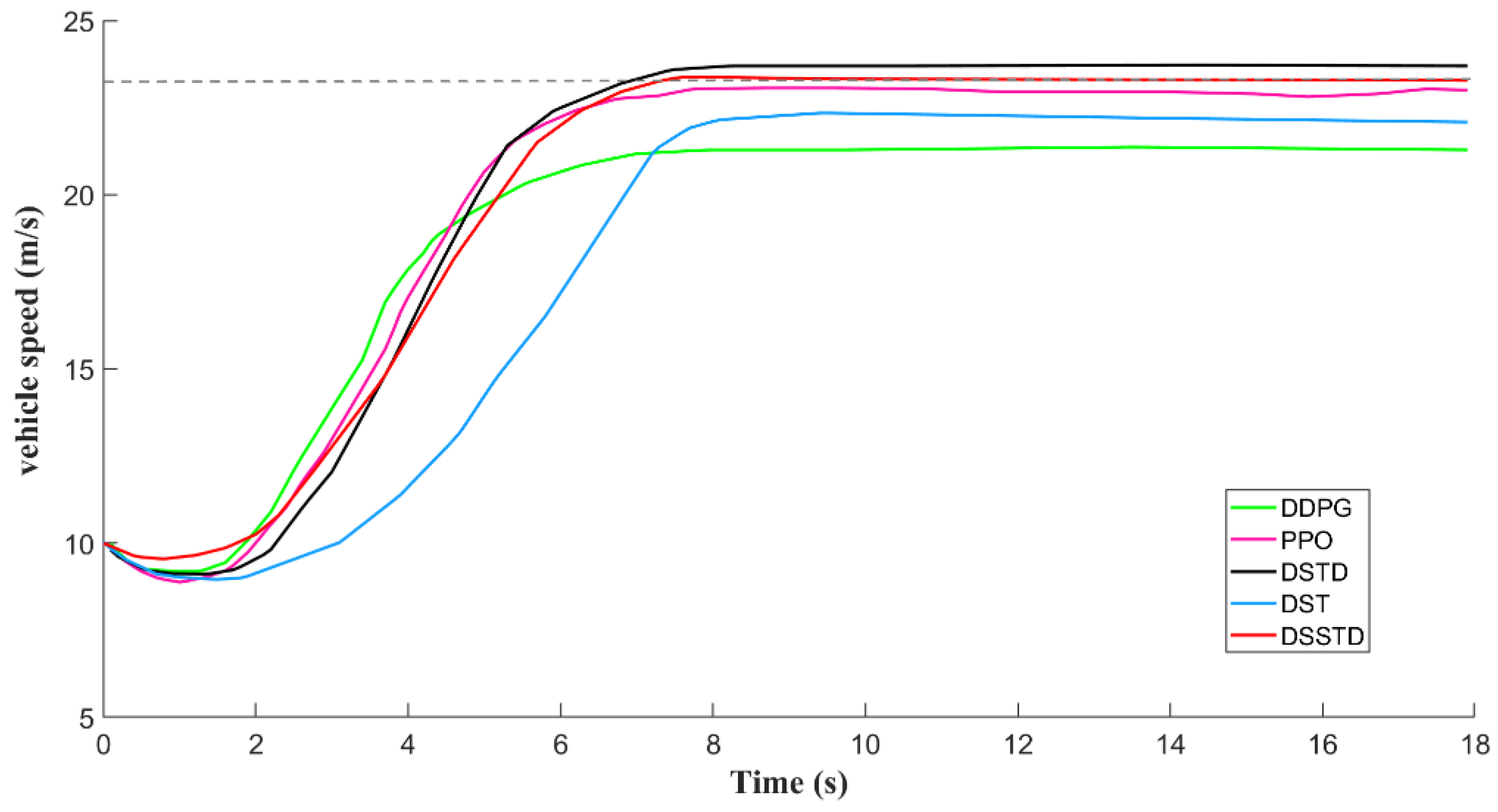
Driving efficiency: The test rounds with an initial speed of 10 m/s were used and the results of changes in their vehicle speeds during testing are shown in Figure 13. We regarded the average speed of the ego vehicle as an indicator to evaluate driving efficiency. The gray dotted line in Figure 13 represents the standard line for the desired speed (also the optimal speed). We hope that the average speed of the ego vehicle can reach the set desired speed value of $v_d$ = 23.0 m/s as quickly as possible, and maintain this stable speed. Among the five strategies, it can be seen that the speed of the traditional DDPG behaved more fluctuant, and finally stabilized at about 22 m/s with the lowest driving efficiency. Compared to PPO, the driving efficiency of PPO was slightly higher, and the speed fluctuation was smaller. This shows that the speed reward item of the traditional algorithm did not finally converge to the optimal value during the training process, resulting in a difference between the average speed and the desired speed.

It should be noted that due to the role of the SR + TM module, the driving safety of the AV is greatly improved, and the corresponding driving efficiency will be slightly affected. However, a slight decrease in the average speed of DST (0.62%) was acceptable since the AV is more inclined to establish safety-oriented driving behaviors. The notable increase in DSTD average speed (23.12 m/s) illustrates that the implementation of DPBRS enhanced the training efficiency of the agent corresponding to the speed related reward function. In addition, regarding driving efficiency, the trained average speed (23.03 m/s) by DSSTD was also closer to the expected one (23 m/s) than the other four. It can be concluded that the DSSTD algorithm is capable of meeting the LC decision expectations in both safety and driving efficiency.

(3)

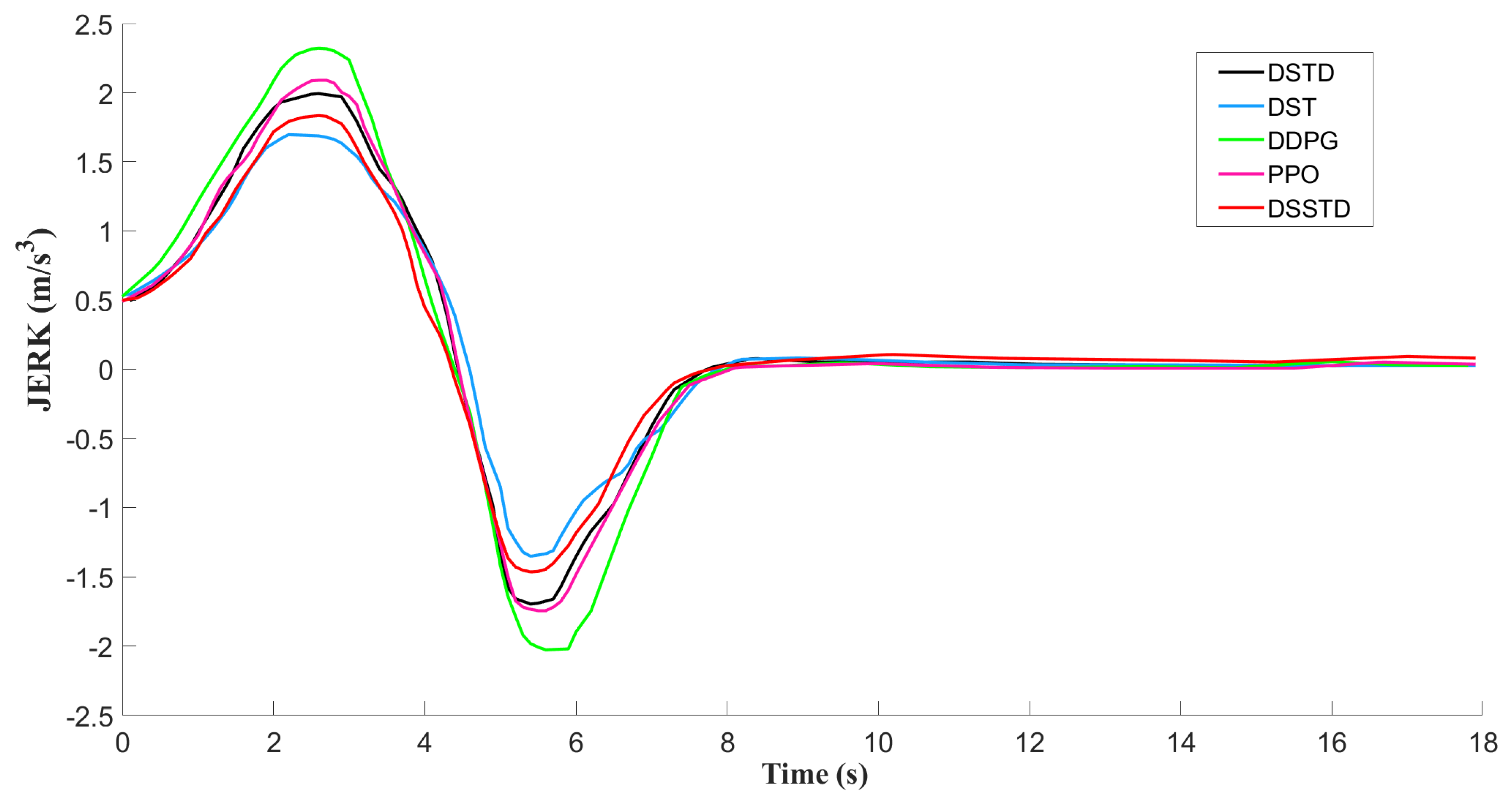
Comfort: For evaluating the comfort of the AV, we will mainly consider the Jerk value, which is defined as the time rate of a change of acceleration. It is clear that a large Jerk value implies a great decrease in driving comfort. According to the reward function described in Section 4, the maximum Jerk was set as $|{\dot{a}}_{cmax}|$ = 2 m/s³. The result of changes in the Jerk values of the five algorithms is shown in Figure 14. The maximum Jerk value of the traditional DDPG was about 2.3 m/s³ slightly higher than the maximum limit. This indicates that the agent cannot fully learn under the specification of the comfort-related reward. The results of PPO and DSTD were both around 2 m/s³. In contrast, that of the DSSTD was 1.81 m/s³, and for DST, it was about 1.65 m/s³, which was much smaller than the other four. Although DST and DSSTD can both have steady and smooth acceleration for comfort evaluation, when considering the testing result of driving efficiency together, the DSSTD was proven to have superior driving performance in agent training.

7. Conclusions

In this paper, a safe and efficient DRL-based autonomous LC decision-making strategy was proposed. We designed an autonomous LC system based on the traditional DDPG algorithm and established a corresponding MDP model. In particular, for driving safety consideration, the Safety Rules (SR) module was adopted to restrict the agent’s actions and the safety prediction (SP) module was used to predict the future states of the AV. Trauma memory (TM) was incorporated to the experience replay, so that the occurrence of collision events in highway scenarios could be reduced. In addition, we developed the reward function by utilizing DPBRS to speed up the optimal strategy learning process. For validation, the proposed method was trained and tested on the dual-computer co-simulation platform. The final simulation results showed that the proposed DSSTD algorithm enabled the AV to achieve 100% LC success rate and 0 collisions/leave the road in the preset LC traffic scenario, which yielded better outcomes than other benchmark algorithms. The minimum distance to the leading vehicle in the same lane was 12.2 m and the minimum TTC was around 1.8 s, which demonstrates that by using the DSSTD algorithm, the driving safety of the AV can be ensured. In addition, the average speed in the test round was 23.03 m/s, which was closer to the desired speed of 23 m/s than other competitors. This indicates that our approach can achieve better performance in driving efficiency. In future work, we will deploy the “weights adjustment mechanism” for the safety and speed related terms in the reward function. The algorithm will be further optimized to improve its robustness to unknown environments and accelerate the learning process of the agent.

References

1. World Health Organization. Global Status Report on Road Safety 2018: Summary; World Health Organization: Geneva, Switzerland, 2018. [Google Scholar]
2. National Highway Traffic Safety Administration (NHTSA). 2016 Fatal Motor Vehicle Crashes. 2017. Available online: https://www.nhtsa.gov/press-releases/usdot-releases-2016-fatal-traffic-crash-data (accessed on 27 March 2021).
3. Eno Center for Transportation. Preparing a Nation for Autonomous Vehicles: Opportunities, Barriers and Policy Recommendations. 2013. Available online: http://www.enotrans.org/wp-content/uploads/wpsc/downloadables/AV-paper.pdf (accessed on 15 January 2022).
4. Thorpe, C.; Herbert, M.; Kanade, T.; Shafter, S. Toward autonomous driving: The cmu navlab. ii. architecture and systems. IEEE Expert 1991, 6, 44–52. [Google Scholar] [CrossRef]
5. Buehler, M.; Iagnemma, K.; Singh, S. (Eds.) The Darpa Urban Challenge: Autonomous Vehicles in City Traffic; Springer: Berlin, Germany, 2009. [Google Scholar]
6. Zhang, M.; Li, N.; Girard, A.; Kolmanovsky, I. A finite state machine based automated driving controller and its stochastic optimization. In Proceedings of the ASME 2017 Dynamic Systems and Control Conference, Tysons, VA, USA, 11–13 October 2017. [Google Scholar]
7. Li, N.; Chen, H.; Kolmanovsky, I.; Girard, A. An explicit decision tree approach for automated driving. In Proceedings of the ASME 2017 Dynamic Systems and Control Conference, Tysons, VA, USA, 11–13 October 2017. [Google Scholar]
8. González, D.; Pérez, J.; Milanés, V. A Review of Motion Planning Techniques for Automated Vehicles. IEEE Trans. Int. Transp. Syst. 2015, 17, 1135–1145. [Google Scholar] [CrossRef]
9. Grigorescu, S.; Trasnea, B.; Cocias, T.; Macesanu, G. A survey of deep learning techniques for autonomous driving. J. Field Robot. 2020, 37, 362–386. [Google Scholar] [CrossRef]
10. Bojarski, M.; del Testa, D.; Dworakowski, D.; Firner, B.; Flepp, B.; Goyal, P.; Jackel, L.D.; Monfort, M.; Muller, U.; Zhang, J. End to end learning for self-driving cars. arXiv 2016, arXiv:1604.07316. [Google Scholar]
11. Kiran, B.R.; Sobh, I.; Talpaert, V.; Mannion, P.; Perez, P. Deep reinforcement learning for autonomous driving: A survey. IEEE Trans. Intell. Transp. Syst. 2021, 1–18. [Google Scholar] [CrossRef]
12. Ronecker, M.P.; Zhu, Y. Deep q-network based decision making for autonomous driving. In Proceedings of the IEEE International Conference on Robotics and Automation Sciences, Montreal, QC, Canada, 20–24 May 2019; pp. 154–160. [Google Scholar]
13. Min, K.; Kim, H.; Huh, K. Deep distributional reinforcement learning based high-level driving policy determination. IEEE Trans. Intell. Veh. 2019, 4, 416–424. [Google Scholar] [CrossRef]
14. Fu, Y.; Li, C.; Yu, F.R.; Luan, T.H.; Zhang, Y. A decision making strategy for vehicle autonomous braking in emergency via deep reinforcement learning. IEEE Trans. Veh. Technol. 2020, 69, 5876–5888. [Google Scholar] [CrossRef]
15. He, X.; Fei, C.; Liu, Y.; Yang, K.; Ji, X. Multi-objective Longitudinal Decision-making for Autonomous Electric Vehicle: A Entropy-constrained Reinforcement Learning Approach. In Proceedings of the 2020 IEEE 23rd International Conference on Intelligent Transportation Systems (ITSC), Rhodes, Greece, 20–23 September 2020; pp. 1–6. [Google Scholar]
16. Chae, H.; Kang, C.M.; Kim, B.D.; Kim, J.; Chung, C.C.; Choi, J.W. Autonomous braking system via deep reinforcement learning. In Proceedings of the 2017 IEEE 20th International Conference on Intelligent Transportation Systems (ITSC), Yokohama, Japan, 16–19 October 2017; pp. 1–6. [Google Scholar]
17. Baheri, A.; Baheri, A.; Nageshrao, S.; Tseng, H.E.; Kolmanovsky, I.; Girard, A.; Filev, D. Deep Reinforcement Learning with Enhanced Safety for Autonomous Highway Driving. In Proceedings of the 2020 IEEE Intelligent Vehicles Symposium (IV), Las Vegas, NV, USA, 20–23 October 2020; pp. 1550–1555. [Google Scholar]
18. Li, G.; Gomez, R.; Nakamura, K.; He, B. Human-centered reinforcement learning: A survey. IEEE Trans. Hum. Mach. Syst. 2019, 49, 337–349. [Google Scholar] [CrossRef]
19. Wang, Z.; Taylor, M. Effective transfer via demonstrations in reinforcement learning: A preliminary study. In Proceedings of the 2016 AAAI Spring Symposia, Stanford University, Palo Alto, CA, USA, 21–23 March 2016. [Google Scholar]
20. Trott, A.; Zheng, S.; Xiong, C.; Socher, R. Keeping your distance: Solving sparse reward tasks using self-balancing shaped rewards. In Proceedings of the Advances in Neural Information Processing Systems, Vancouver, BC, Canada, 8–14 December 2019; pp. 10376–10386. [Google Scholar]
21. Lillicrap, T.P.; Hunt, J.J.; Pritzel, A.; Heess, N.; Erez, T.; Tassa, Y.; Silver, D.; Wierstra, D. Continuous Control with Deep Reinforcement Learning. 2015. Available online: http://arxiv.org/abs/1509.02971 (accessed on 15 January 2022).
22. Ye, Y.; Zhang, X.; Sun, J. Automated vehicle’s behavior decision making using deep reinforcement learning and high-fidelity simulation environment. Transp. Res. C Emerg. Technol. 2019, 107, 155–170. [Google Scholar] [CrossRef] [Green Version]
23. Liang, X.; Wang, T.; Yang, L.; Xing, E. Cirl: Controllable imitative reinforcement learning for vision-based self-driving. In Proceedings of the European Conference on Computer Vision (ECCV), Munich, Germany, 8–14 September 2018; pp. 584–599. [Google Scholar]
24. Wang, Q.; Zhuang, W.; Wang, L.; Ju, F. Lane Keeping Assist for an Autonomous Vehicle Based on Deep Reinforcement Learning. In Proceedings of the WCX SAE World Congress Experience, Detroit, MI, USA, 21–24 April 2020. [Google Scholar]
25. Tang, Y. Towards Learning Multi-Agent Negotiations via Self-Play. 2019. Available online: https://arxiv.org/abs/2001.10208 (accessed on 15 January 2022).
26. Karaduman, O.; Eren, H.; Kurum, H.; Celenk, M. Interactive risky behavior model for 3-car overtaking scenario using joint Bayesian network. In Proceedings of the 2013 IEEE Intelligent Vehicles Symposium (IV), Gold Coast, Australia, 23–26 June 2013; pp. 1279–1284. [Google Scholar]
27. Bouton, M.; Nakhaei, A.; Fujimura, K.; Kochenderfer, M.J. Safe Reinforcement Learning with Scene Decomposition for Navigating Complex Urban Environments. In Proceedings of the IEEE Intelligent Vehicles Symposium (IV), Paris, France, 9–12 June 2019; pp. 1469–1476. [Google Scholar]
28. Wen, L.; Duan, J.; Li, S.E.; Xu, S.; Peng, H. Safe Reinforcement Learning for Autonomous Vehicles through Parallel Constrained Policy Optimization. 2020. Available online: https://arxiv.org/abs/2003.01303 (accessed on 15 January 2022).
29. Kamran, D.; Lopez, C.F.; Lauer, M.; Stiller, C. Risk-Aware High-level Decisions for Automated Driving at Occluded Intersections with Reinforcement Learning. In Proceedings of the 2020 IEEE Intelligent Vehicles Symposium (IV), Las Vegas, NV, USA, 23 June 2020; pp. 1205–1212. [Google Scholar]
30. Peng, H.; Du, B.; Liu, M.; Liu, M.; He, L. Dynamic graph convolutional network for long-term traffic flow prediction with reinforcement learning. Inf. Sci. 2021, 578, 401–416. [Google Scholar] [CrossRef]
31. Buhet, T.; Wirbel, E.; Perrotton, X. Conditional vehicle trajectories prediction in carla urban environment. In Proceedings of the IEEE International Conference on Computer Vision Workshops, Seoul, Korea, 27–28 October 2019. [Google Scholar]
32. Vasquez, R.; Farooq, B. Multi-Objective Autonomous Braking System using Naturalistic Dataset. In Proceedings of the 2019 IEEE Intelligent Transportation Systems Conference (ITSC), Auckland, New Zealand, 27–30 October 2019; pp. 4348–4353. [Google Scholar]
33. Kohler, S.; Schreiner, B.; Ronalter, S.; Doll, K.; Zindler, K. Autonomous evasive maneuvers triggered by infrastructure-based detection of pedestrian intentions. In Proceedings of the 2013 IEEE Intelligent Vehicles Symposium (IV), Gold Coast, Australia, 23–26 June 2013; pp. 519–526. [Google Scholar]
34. Brannstrom, M.; Coelingh, E.; Sjoberg, J. Model-based threat assessment for avoiding arbitrary vehicle collisions. IEEE Trans. Intell. Transp. Syst. 2010, 11, 658–669. [Google Scholar] [CrossRef]
35. Mnih, V.; Kavukcuoglu, K.; Silver, D.; Rusu, A.A.; Veness, J.; Bellemare, M.G.; Graves, A.; Riedmiller, M.; Fidjeland, A.K.; Ostrovski, G.; et al. Human-level control through deep reinforcement learning. Nature 2015, 518, 529. [Google Scholar] [CrossRef] [PubMed]
36. Okudo, T.; Yamada, S. Subgoal-based Reward Shaping to Improve Efficiency in Reinforcement Learning. IEEE Access 2021, 9, 97557–97568. [Google Scholar] [CrossRef]
37. Marom, O.; Rosman, B.S. Belief reward shaping in reinforcement learning. In Proceedings of the 32nd AAAI Conference on Artificial Intelligence, New Orleans, LA, USA, 2–7 February 2018; AAAI Press: Palo Alto, CA, USA; pp. 3762–3769. [Google Scholar]
38. Demir, A.; Cilden, E.; Polat, F. Landmark based reward shaping in reinforcement learning with hidden states. In Proceedings of the 18th International Conference on Autonomous Agents and Multi Agent Systems, Montreal, QC, Canada, 13–17 May 2019; pp. 1922–1924. [Google Scholar]
39. Paul, S.; Baar, J.V.; Roy-Chowdhury, A.K. Learning from trajectories via subgoal discovery. Adv. Neural Inf. Processing Syst. 2019, 32, 8411–8421. [Google Scholar]
40. Hoel, C.J.; Driggs-Campbell, K.; Wolff, K.; Laine, L.; Kochenderfer, M.J. Combining Planning and Deep Reinforcement Learning in Tactical Decision Making for Autonomous Driving. IEEE Trans. Int. Veh. 2020, 5, 294–305. [Google Scholar] [CrossRef] [Green Version]
41. Hugle, M.; Kalweit, G.; Mirchevska, B.; Werling, M.; Boedecker, J. Dynamic Input for Deep Reinforcement Learning in Autonomous Driving. In Proceedings of the 2019 IEEE/RSJ International Conference on Intelligent Robots and Systems (IROS), Macau, China, 3–8 November 2019; pp. 7566–7573. [Google Scholar]
42. Mnih, V.; Kavukcuoglu, K.; Silver, D.; Graves, A.; Antonoglou, I.; Wierstra, D.; Riedmiller, M. Playing Atari with deep reinforcement learning. arXiv 2013, arXiv:1312.5602. [Google Scholar]
43. Treiber, M.; Hennecke, A.; Helbing, D. Congested traffic states in empirical observations and microscopic simulations. Phys. Rev. E 2000, 62, 1805. [Google Scholar] [CrossRef] [PubMed] [Green Version]
44. Kesting, A. General lane-changing model MOBIL for car-following models. Transp. Res. Rec. 2007, 1999, 86–94. [Google Scholar] [CrossRef] [Green Version]
45. Liu, T.; Huang, B.; Mu, X.; Zhao, F.; Cao, D. A Comparative Analysis of Deep Reinforcement Learning-Enabled Freeway Decision-Making for Automated Vehicles. 2020. Available online: http://arxiv.org/abs/2008.01302 (accessed on 15 January 2022).
46. Treiber, M.; Kesting, A.; Thiemann, C. Traffic Flow Dynamics: Data, Models and Simulation; Springer Science & Business Media: Berlin, Germany, 2013. [Google Scholar]
47. Van Der Horst, A.R.A. A Time-Based Analysis of Road User Behaviour in Normal and Critical Encounters; TNO Institute for Perception: Soesterberg, The Netherlands, 1990. [Google Scholar]
48. Xu, J.; Pei, X.; Lv, K. Decision-Making for Complex Scenario using Safe Reinforcement Learning. In Proceedings of the 2020 4th CAA International Conference on Vehicular Control and Intelligence (CVCI), Hangzhou, China, 18–20 December 2020; pp. 1–6. [Google Scholar]
49. Ng, A.Y. Policy invariance under reward transformations: Theory and application to reward shaping. In Proceedings of the Sixteenth International Conference on Machine Learning, Bled, Slovenia, 27–30 June 1999; pp. 278–287. [Google Scholar]
Figure 1. Markov decision process.
Mathematics 10 01551 g001
Figure 2. DDPG algorithm flowchart.
Mathematics 10 01551 g002
Figure 3. AV lane changing process.
Mathematics 10 01551 g003
Figure 4. Training scenario.
Mathematics 10 01551 g004
Figure 5. System architecture of the proposed RL algorithm.
Mathematics 10 01551 g005
Figure 6. Safety Rules module.
Mathematics 10 01551 g006
Figure 7. Safety Prediction module.
Mathematics 10 01551 g007
Figure 8. RL co-simulation platform.
Mathematics 10 01551 g008
Figure 9. Single step time of the co-simulation platform.
Mathematics 10 01551 g009
Figure 10. The evaluation of the proposed DRL model. (a) the average Q value curve for evaluating the stability of DSSTD model. (b) the loss value curve for evaluating the stability of DSSTD model.
Mathematics 10 01551 g010
Figure 11. The average reward curve of the proposed RL algorithm and the traditional RL algorithm.
Mathematics 10 01551 g011
Figure 12. Distribution of the TTC of the proposed RL algorithm and the traditional RL algorithm.
Mathematics 10 01551 g012
Figure 13. The speed curve of the AV in the test round.
Mathematics 10 01551 g013
Figure 14. The Jerk curve of the AV in the test round.
Mathematics 10 01551 g014