Brauer Configuration Algebras Arising from Dyck Paths

Abstract

The enumeration of Dyck paths is one of the most remarkable problems in Catalan combinatorics. Recently introduced categories of Dyck paths have allowed interactions between the theory of representation of algebras and cluster algebras theory. As another application of Dyck paths theory, we present Brauer configurations, whose polygons are defined by these types of paths. It is also proved that dimensions of the induced Brauer configuration algebras and the corresponding centers are given via some integer sequences related to Catalan triangle entries.

1. Introduction

In the last few years, several combinatorial objects have allowed the research development of the theory of representation of algebras. For instance, the number of triangulations of a polygon with $n+3$ sides, or the number of Dyck paths of length $2n$ in the plane connecting the origin with a point $P=(2n,0)$. Edges in these paths are either rises (linking points $(x,y)$ and $(x+1,y+1)$ in ${\mathbb{N}}^2$) or falls (connecting points $(x,y)$ and $(x+1,y-1)$ in ${\mathbb{N}}^2$) [1]. Caldero, Chapoton, and Schiffler [2] proved that any triangulation T of an $(n+3)$-polygon defines a category ${\mathrm{mod}}_{\mathbb{F}}{Q}_T$ of finitely generated modules over a path algebra $\mathbb{F}{Q}_T$ induced by a quiver $Q_T$ arisen from the triangulation T. They also proved that ${\mathrm{mod}}_{\mathbb{F}}{Q}_T$ can be identified with the category of diagonals defining the triangulation.

Following the ideas by Caldero et al., Cañadas et al. [3] introduced a categorical equivalence between a category ${\mathcal{C}}_{2n}$ of Dyck paths and a category of representations $\mathrm{rep}{\mathbb{A}}_{n-1}$ of a quiver of Dynkin type ${\mathbb{A}}_{n-1}$. These approaches allow obtaining formulas for cluster variables of type $\mathbb{A}$ and frieze patterns in terms of Dyck paths and perfect matchings of some snake graphs. It is worth pointing out that finding formulas of these types is a significant problem in the cluster algebras theory.

On the other hand, Brauer configuration algebras (BCAs) are bound quiver algebras introduced by Green and Schroll in [4]. The structure of the indecomposable projective modules over these types of algebras is given by some combinatorial data, which are also used to determine their dimension. BCAs were used by Espinosa [5] to categorify integer sequences in the sense of Ringel and Fahr, i.e., the numbers in these sequences can be considered as invariants of objects in a category. They are also helpful in several fields of applied mathematics (cryptography, graph energy theory, algebraic combinatorics, etc. [6,7,8,9]).

Contributions

This paper establishes a connection between Dyck paths and Brauer configuration algebras researches by proving that Dyck paths define suitable words associated with polygons in a Brauer configuration. We introduce new Catalan–Brauer configurations (CBCs) obtaining formulas for the dimensions of the corresponding BCAs and their centers. To do that, we introduce an integer sequence $S=\left\{{\mathfrak{h}}_{x,j}^i\right\}$ whose properties allow obtaining formulas relating its elements with entries of the Catalan triangle. Thus, the approach allows giving another manifestation of Catalan numbers via BCAs.

Figure 1 shows how Brauer configuration algebras and Dyck paths theories are related to the main results presented in this paper.

The organization of this paper goes as follows; the main definitions and notation are given in Section 2, we recall the definitions and notation used throughout the document. In particular, we recall notions of Dyck paths, Catalan triangle, and Brauer configuration algebra (Section 2.2). In Section 3, we give our main results. We introduce an integer sequence whose elements are related to the entries of the Catalan triangle. The numbers in this sequence allow giving a formula to compute the dimension of some Brauer configuration algebras, whose polygons are defined by Dyck paths. The concluding remarks are given in Section 4.

2. Background and Related Work

This section is devoted to reminding the basic notation and results concerning Dyck paths, the Catalan triangle, and Brauer configuration algebras, which are helpful for a better understanding of the paper.

2.1. Dyck Paths and Catalan Triangle

In this section, we make a brief review on Dyck paths and the Catalan triangle [1,10].

Dyck paths, as defined in the introduction, were enumerated by Stanley [1], who proved that there are $C_n=\frac{1}{n+1}\left(\genfrac{}{}{0pt}{}{2n}{n}\right)$ Dyck paths of length $2n$, where $C_n$ denotes the nth Catalan number. ${\mathfrak{p}}_{2n}=\{P\mid P\mathrm{is}\mathrm{a}\mathrm{Dyck}\mathrm{path},|P|=2n\}$.

For $u\ge 0$ and $0\le v\le u$. The Catalan’s triangle is an integer array whose entries $C(u,v)$ are given by the formula [10].

$$C(u,v)=\frac{u-v+1}{u+1}\left(\genfrac{}{}{0pt}{}{u+v}{v}\right),u\ge 0,\mathrm{and}0\le v\le u.$$

(1)

There are many ways of finding Catalan triangle entries in the specialized literature. For instance, the array (3) gives such numbers according to the recurrence (2). Such a recurrence was found by Cañadas et al. [3] via some seed vectors associated with positive integral diamonds of type ${\mathbb{A}}_n$ arising from the theory of integer friezes.

$${\displaystyle {\mathfrak{p}}_{x,y}=\left\{\begin{array}{c}{\displaystyle {\mathfrak{p}}_{1,1}={\mathfrak{p}}_{1,2}=1,}\hfill \\ {\displaystyle \sum _{i=y-1}^x{\mathfrak{p}}_{x-1,i},}\hfill & \mathrm{if}y>1,\mathrm{and}x>1,\hfill \\ {\displaystyle \sum _{i=1}^x{\mathfrak{p}}_{x-1,i},}\hfill & \mathrm{if}y=1,\mathrm{and}x>1.\hfill \end{array}\right.}$$

(2)

$$\begin{array}{ll}{\mathfrak{p}}_{1,2}=1& {\mathfrak{p}}_{1,1}=1\\ {\mathfrak{p}}_{2,3}& {\mathfrak{p}}_{2,2}{\mathfrak{p}}_{2,1}\\ {\mathfrak{p}}_{3,4}& {\mathfrak{p}}_{3,3}{\mathfrak{p}}_{3,2}{\mathfrak{p}}_{3,1}\\ {\mathfrak{p}}_{4,5}& {\mathfrak{p}}_{4,4}{\mathfrak{p}}_{4,3}{\mathfrak{p}}_{4,2}{\mathfrak{p}}_{4,1}\\ ⋮& \ddots \end{array}$$

(3)

2.2. Brauer Configuration Algebras

Green and Schroll introduced the notion of a BCA (Brauer Configuration Algebra). The authors refer the interested reader to [4,11] for a more detailed study of BGAs (Brauer Graph Algebras) and BCAs. In the sequel, we make a brief description of the structure of these algebras.

A BCA ${\Lambda }_{\Gamma }$ is a bound quiver algebra induced by a Brauer configuration $\Gamma =({\Gamma }_0,{\Gamma }_1,\mu ,\mathcal{O})$ of sets, with the functions and orders satisfying the following conditions:

• Elements of the set ${\Gamma }_0$ are called vertices;
• ${\Gamma }_1$ consists of multisets called polygons, which consist of vertices that can be repeated. Moreover, if $U\in {\Gamma }_1$. Then $\left|U\right|>1$;
• $\mu$ denotes a function from the set of vertices to the set of positive integers. Green and Schroll called this function the multiplicity function, associated with the Brauer configuration $\Gamma$;
• If a vertex h in a polygon W occurs t times. Then, we will write $occ(h,W)=t$. $val\left(h\right)={\displaystyle \sum _{W\in {\Gamma }_1}}occ(h,W)$ is said to be the valency of the vertex h, which is said to be non-truncated
  if $val\left(h\right)\mu \left(h\right)\ne 1$ (otherwise, it is non-truncated). We let $S_h$ denote the maximal set of polygons containing a non-truncated vertex. If $S_h=\{U_{i_1},U_{i_2},\dots ,U_{i_m}\}$. Then $S_h$ is endowed with a well-order <, which allows writing $S_h$ in the following form:

  $$U_{i_1}^{h_1}<U_{i_2}^{h_2}<\dots <U_{i_m}^{h_m},h_{i_s}>0.$$

  (4)
  The symbol $U_{i_j}^x$ is used to denote that $occ(h,U_{i_j})=x$. In successor sequences $U^x$ denotes a subsequence of length x with the form:

  $$\underset{x-times}{\underbrace{U<U\dots <U}}$$

  (5)
  The set $(S_h,<)$ is said to be the successor sequence associated with the vertex h. Note that if $U_i<U_j$ is a covering in $S_h$ and $h^{\prime }\in U_i\cap U_j$ with $h^{\prime }\ne h$ then the relation $U_i<U_j$ also appears in the sequence $S_{h^{\prime }}$.

In this work, it is assumed that each polygon $U_i\in {\Gamma }_1$ is given by a word $w_{U_i}$ of the form

$$\begin{array}{cc}\hfill w_{U_i}& ={\alpha }_1^{s_1}{\alpha }_2^{s_2}\dots {\alpha }_{t-1}^{s_{t-1}}{x}_t^{s_t}\hfill \end{array}$$

(6)

where for each i, $1\le i\le t$, ${\alpha }_i$ is a vertex, and $s_i=occ({\alpha }_i,U_i)$.

Algorithm 1 is a short version of an algorithm introduced in [6] by Cañadas et al. to construct a Brauer configuration algebra.

Algorithm 1: Building a BCA

Input.$\Gamma =({\Gamma }_0,{\Gamma }_1,\mu ,\mathcal{O})$. Output. The BCA ${\Lambda }_{\Gamma }=\mathbb{F}{Q}_{\Gamma }/I_{\Gamma }$ induced by the BC $\Gamma$. Remove truncated vertices. Define the Brauer quiver $Q_{\Gamma }=(Q_0,Q_1,s,t)$, such that (a) $Q_0={\Gamma }_1$, (b) For each covering $U_i\le U_{i+1}$ contained in a successor sequence $S_{\alpha }$, define an arrow $a^{\alpha }$ for which $s\left(a^{\alpha }\right)=U_i$, and $t\left(a^{\alpha }\right)=U_{i+1}$, (c) To each ordered successor sequence $S_{\alpha }$ define a special cycle $C_{\alpha }$ associated with a vertex $\alpha$ by adding a relation $r_{\alpha }$ of the form $U_{\max S_{\alpha }}<U_{\max S_{\alpha }}$. Define the path algebra $\mathbb{F}{Q}_{\Gamma }$. Define an admissible ideal $I_{\Gamma }$ generated by the following relations: (a) $a^{\alpha }{a}^{{\alpha }^{\prime }}$, if $\alpha ,{\alpha }^{\prime }\in {\Gamma }_0$, $\alpha \ne {\alpha }^{\prime }$, $a^{\alpha }{a}^{{\alpha }^{\prime }}\in \mathbb{F}{Q}_{\Gamma }$, (b) $C_{\alpha }^{\mu \left(\alpha \right)}f$, if f is the first arrow of a special cycle $C_{\alpha }$ associated with $\alpha$, (c) ${\left(l^{\alpha }\right)}^{\mu \left(\alpha \right)+1}$, if l is a loop associated with a non-truncated vertex $\alpha \in {\Gamma }_0$, and $val\left(\alpha \right)=1$. (d) $C_{\alpha }^{\mu \left(\alpha \right)}-C_{{\alpha }^{\prime }}^{\mu \left({\alpha }^{\prime }\right)}$, for any pair of special cycles associated with vertices $\alpha ,{\alpha }^{\prime }\in U$, $U\in {\Gamma }_1$. Define the Brauer configuration algebra ${\Lambda }_{\Gamma }=\mathbb{F}{Q}_{\Gamma }/I_{\Gamma }$. The union of classes of proper prefixes of special cycles with classes of special cycles provide an $\mathbb{F}$ basis $\mathcal{B}$ of ${\Lambda }_{\Gamma }$.

Later on, if there is not possibility of confusion, we will assume notations Q (for a quiver), I (for an admissible ideal) and $\Lambda$ (for a Brauer configuration algebra).

Theorem 1 provides algebraic properties of BCAs [4].

Theorem 1 

([4], Theorem B, Propositions 2.7, 3.2 and 3.5, Theorem 3.10, Corollary 3.12 ). Let $\Lambda =\mathbb{F}Q/I$ be a Brauer configuration algebra induced by a Brauer configuration $\Gamma =({\Gamma }_0,{\Gamma }_1,\mu ,\mathcal{O})$.

1. 

There is a bijection between the set of indecomposable projective modules over Λ and ${\Gamma }_1$;

2. 

If $P_V$ is an indecomposable projective module over a BCA Λ defined by a polygon V in ${\Gamma }_1$. Then $\mathrm{rad}{P}_V={\displaystyle \sum _{i=1}^r}{U}_i$, where $U_i\cap U_j$ is a simple Λ-module for any $1\le i,j\le r$, and r is the number of (non-truncated) vertices of V;

3. 

I is admissible, whereas Λ is a multiserial symmetric algebra. Moreover, if Γ is connected, then Λ is indecomposable as an algebra;

4. 

If $\mathrm{rad}P$ ($\mathrm{soc}P$) denotes the radical (socle) of an indecomposable projective module P, and ${\mathrm{rad}}^{2}P\ne 0$. Then, the number of summands in the heart $\mathrm{rad}P/\mathrm{soc}P$ of P equals the number of non-truncated vertices of the polygons in Γ corresponding to P counting repetitions;

5. 

If ${\Lambda }_{\Gamma }$ and ${\Lambda }_{{\Gamma }^{\prime }}$ are BCAs, induced by Brauer configurations $\Gamma =({\Gamma }_0,{\Gamma }_1,\mu ,\mathcal{O})$, and ${\Gamma }^{\prime }=({\Gamma }_0\backslash \left\{h\right\},{\Gamma }_1\backslash V\cup V^{\prime },\mu ,\mathcal{O})$, where $V^{\prime }=V\backslash \left\{h\right\}$, $\left|V\right|\ge 3$, and $val\left(h\right)\mu \left(h\right)=1$. Then, ${\Lambda }_{\Gamma }$ is isomorphic to ${\Lambda }_{{\Gamma }^{\prime }}$.

Green and Schroll in [4] proved that the dimension of a Brauer configuration algebra is given by the following formula.

$${\dim }_{\mathbb{F}}\Lambda =2\left|{\Gamma }_1\right|+\sum _{i\in {\Gamma }_0}val\left(i\right)(\mu \left(i\right)val\left(i\right)-1).$$

(7)

Sierra [12] obtained the next formula for the dimension of the center of a connected Brauer configuration algebra ${\Lambda }_{\Gamma }$ with radical square different from zero.

$$\begin{array}{cc}\hfill {\dim }_{\mathbb{F}}Z(\Lambda )& =1+\sum _{\alpha \in {\Gamma }_0}\mu \left(\alpha \right)+|{\Gamma }_1|-|{\Gamma }_0|+\#\left(LoopsQ\right)-|{\mathcal{C}}_{\Gamma }|,\hfill \end{array}$$

(8)

where $|{\mathcal{C}}_{\Gamma }|=\{\alpha \in {\Gamma }_0\mid val\left(\alpha \right)=1,\mathrm{and}\mu \left(\alpha \right)>1\}$.

As an example, we use compositions of the number 3 to define a Brauer configuration $\Delta =({\Delta }_0,{\Delta }_1,\mu ,\mathcal{O})$ for which;

• ${\Delta }_0=\{1,2,3\}$;
• ${\Delta }_1=\{U_1=\{3,1,1,1\},U_2=\{2,1\},U_3=\{1,2\}\}$;
• $\mu \left(1\right)=\mu \left(2\right)=1$, $\mu \left(3\right)=2$;
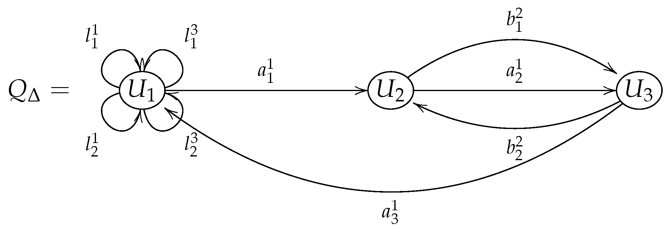
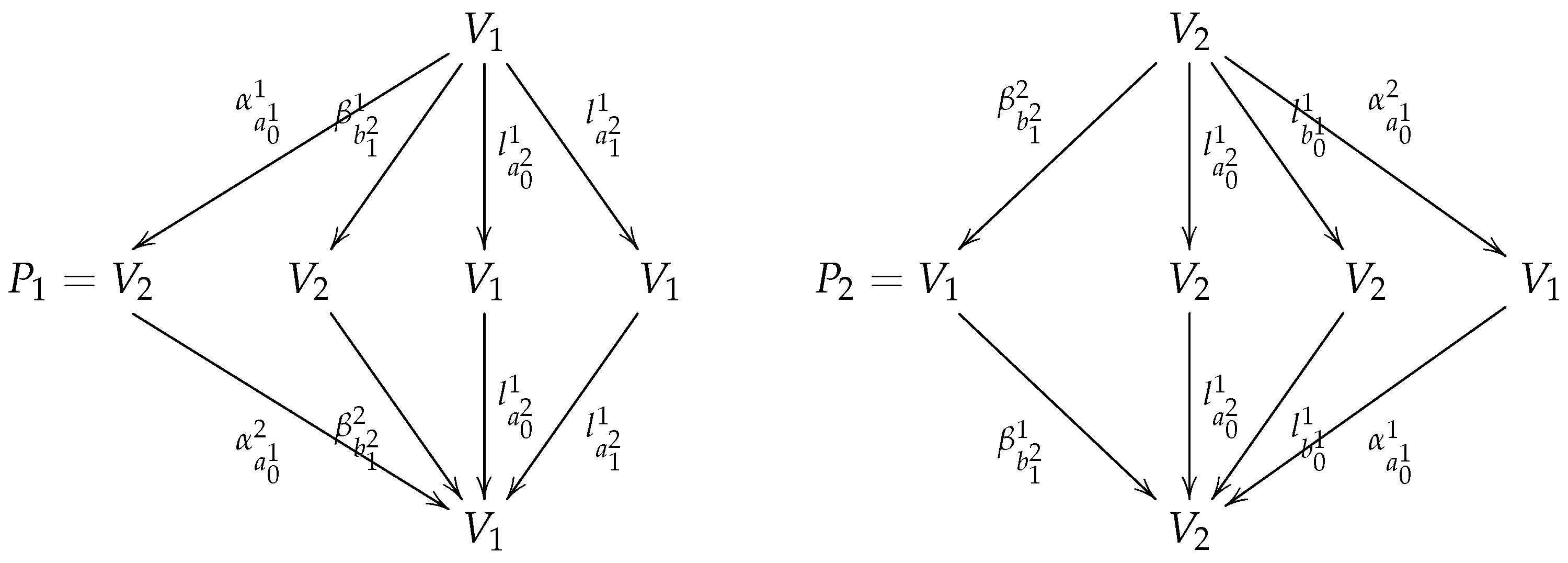
• Successor sequences: $S_1=U_1^{\left(3\right)}<U_2<U_3$, $S_2=U_2<U_3$, $S_3=U_1$;
• $val\left(1\right)=5$, $val\left(2\right)=2$, $val\left(3\right)=1$;
• $|{\Delta }_0|=3$, $|{\Delta }_1|=3$, $|{\mathcal{C}}_{\Delta }|=1$;
• ${\dim }_{\mathbb{F}}{\Lambda }_{\Delta }=29$;
• ${\dim }_{\mathbb{F}}Z\left({\Lambda }_{\Delta }\right)=8$.

The following Figure 2 shows the Brauer quiver $Q_{\Delta }$.

The admissible ideal $I_{\Delta }$ is generated by the following relations (a and $a^{\prime }$ denote first arrows of special cycles $C_{\alpha }$ associated with a vertex $\alpha$).

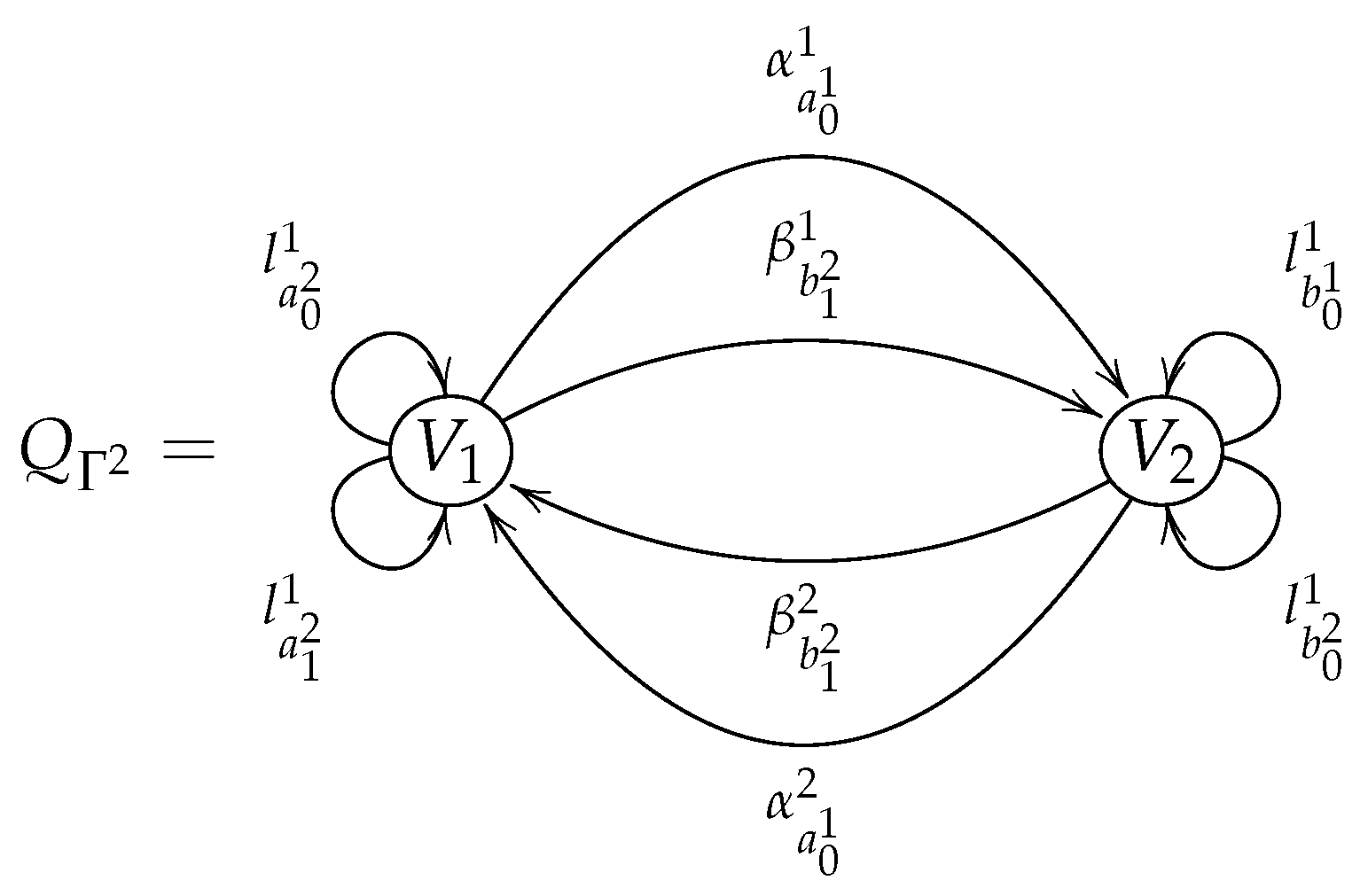
• $l_i^1{l}_j^3$, ${\left(l_i^1\right)}^2$, ${\left(l_i^3\right)}^2$, for all possible values of i and j;
• $l_i^3{a}_1^1$, $a_1^1{b}_1^2$, $b_1^2{a}_3^1$, $C_1^{1}a$, $C_2^1{a}^{\prime }$, $C_1^1\sim C_2^1$, for all possible special cycles associated with vertices 1 and 2.

3. Main Results

The results in this section allow establishing interactions between Catalan combinatorics via Dyck paths and Brauer configuration algebras. It is proved that indecomposable projective modules over some Brauer configuration algebras define Dyck paths. We compute the dimension of these algebras and their corresponding centers.

3.1. Dyck Paths Arising from Brauer Configuration Algebras

For a fixed integer x, and sets of letters

$$F_x={\left\{{\mathfrak{a}}_{x_1}^{x_2}\right\}}_{0\le x_1\le x-1,x_1<x_2\le x},G_x={\left\{{\mathfrak{b}}_{x_1}^{x_2}\right\}}_{0\le x_1\le x-1,x_1<x_2\le x}.$$

(9)

It is defined a Brauer configuration ${\Gamma }^x=({\Gamma }_0^x,{\Gamma }_1^x,{\mu }^x,{\mathcal{O}}^x)$, where

$${\Gamma }_0^x=F_x\cup G_x.$$

(10)

If a product or concatenation c is defined on the set ${\Gamma }_0^x$ in the following fashion:

$$c\left(\delta \right)=\left\{\begin{array}{cc}{\mathfrak{a}}_p^{q+1},\hfill & \mathrm{if}\delta ={\mathfrak{a}}_p^q,\hfill \\ {\mathfrak{b}}_p^q,\hfill & \mathrm{if}\delta ={\mathfrak{a}}_p^q,\hfill \\ {\mathfrak{a}}_{p+1}^{q+1},\hfill & \mathrm{if}\delta ={\mathfrak{b}}_p^q,\hfill \\ {\mathfrak{b}}_{p+1}^q,\hfill & \mathrm{if}\delta ={\mathfrak{b}}_p^q,\hfill \end{array}\right.$$

(11)

for suitable integers p and q.

Then the word $w_V$ associated with a polygon $V\in {\Gamma }_1^x$ has the form $w_V={\delta }_1\dots {\delta }_{2n}={\displaystyle \prod _{h=1}^{2n}}{\delta }_h$, where ${\delta }_1={\mathfrak{a}}_0^1$ and ${\delta }_q=c\left({\delta }_{q-1}\right)$.

The orientation ${\mathcal{O}}^x$ is defined by an order < satisfying the following conditions: Successor sequences associated with vertices can be defined by adopting the following relation

$$\begin{array}{cc}\hfill V& <V^{\prime }\mathrm{if}\mathrm{and}\mathrm{only}\mathrm{if}\mathrm{there}\mathrm{exists}\mathrm{a}\mathrm{positive}\mathrm{integer}r\mathrm{such}\mathrm{that}\hfill \\ \hfill {\mathfrak{N}}_V^{r_g}& ={\mathfrak{N}}_{V^{\prime }}^{r_g}\mathrm{if}0<r_g<r,\hfill \\ \hfill {\mathfrak{N}}_{V^{\prime }}^{r_g}& <{\mathfrak{N}}_V^{r_g}\mathrm{if}{r}_g=r.\hfill \end{array}$$

(12)

where ${\mathfrak{N}}_V^{r_g}$ is the number of $\mathfrak{a}$ words appearing before the first occurrence of an $r_g$-$\mathfrak{b}$ word in V.

If no confusion arises, henceforth, we will write polygons in terms of their corresponding words. In successor sequences polygons $V_i\in {\Gamma }_1^x$ are (linearly) ordered in the form $V_1<V_2<\dots$, where

$$V_1=\prod _{q=1}^n{\mathfrak{a}}_0^q\prod _{p=0}^n{\mathfrak{b}}_p^x,V_2=\prod _{q=1}^{n-1}{\mathfrak{a}}_0^q\left({\mathfrak{b}}_0^{n-1}{\mathfrak{a}}_1^n\right)\prod _{p=1}^{n-1}{\mathfrak{b}}_p^x,\dots$$

(13)

Remark 1.

It is worth pointing out that under these circumstances, it is easy to prove that there is a bijection between words of type $V_i$ and Dyck paths of type ${\mathfrak{p}}_{2n}$.

The multiplicity function ${\mu }^x:{\Gamma }_0^x\to {\mathbb{N}}^{+}$ is defined in such a way that

$${\mu }^x\left(\delta \right)=2,\mathrm{if}val\left(\delta \right)=1,{\mu }^x\left(\delta \right)=1,\mathrm{otherwise}.$$

(14)

Brauer configurations of type ${\Gamma }^x$ are called Catalan–Brauer configurations. We note that, if $V\in {\Gamma }_1^x$, then $occ({\mathfrak{a}}_{x_1}^{x_2},V)$ is given by an entry of the $(\frac{x_1(2x-x_1)}{2}+x_2-\frac{1}{2})$-row of the $\frac{x(x+1)}{2}\times {\mathfrak{p}}_{x,2}$-matrix $A_x=\left(a_{i,j}^x\right)$ shown in Figure 3 (see identities (2)). On the other hand, the same row in a matrix $B_x=\left(b_{i,j}^x\right)$ of the same size gives $occ({\mathfrak{b}}_{x_1}^{x_2},V)$. Note that, $A_1=B_1=\left(1\right)$.

Entries of Matrix $A_{x-1}^{p,{\mathfrak{p}}_{(x-1,p+1)}}=\left(a_{i,j}^{x-1,p}\right)$ are given by the following identities:

$$a_{i,j}^{x-1,p}=\left\{\begin{array}{cc}{a}_{i,j}^{x-1},\hfill & \mathrm{if}i>p,\hfill \\ 0,\hfill & \mathrm{otherwise},\hfill \end{array}\right.$$

(15)

where $0\le p\le x-1$.

Entries $b_{i,j}^{x-1,p}\in B_{x-1}^{p,{\mathfrak{p}}_{(x-1,p+2)}}$ are given by the same formulas for $-1\le p\le x-1$.

Paths in $\mathbb{F}Q$ associated with the Brauer quiver induced by ${\Gamma }^x$ are given by words of the form ${\displaystyle \prod _{h=1}^k}{a}_{q_h}^p$ or ${\displaystyle \prod _{h=1}^{k^{\prime }}}{b}_{q_h^{\prime }}^{p^{\prime }}$. In this case, $a_{p,q_r}^x=b_{p^{\prime },q_{r^{\prime }}^{\prime }}^x=1$ with $q_r<q_{r+1}$, $q_r^{\prime }<q_{r^{\prime }+1}^{\prime }$, $1\le q_r,q_{r^{\prime }}^{\prime }\le {\mathfrak{p}}_{x,2}$. And $1\le p\le \frac{x(x+1)}{2}$.

${\left(a_q^p\right)}^2$ and ${\left(b_{q^{\prime }}^{p^{\prime }}\right)}^2$ denote loops associated with vertices $\delta$ for which $val\left(\delta \right)=1$.

Special cycles $C_p$ associated with a given non-truncated vertex ${\delta }_p$ are given by the following identities:

$$C_p=\left\{\begin{array}{cc}{\displaystyle \prod _{h=t}^k}{a}_{q_h}^p{\displaystyle \prod _{h=1}^{t-1}}{a}_{q_h}^p,\hfill & a_{p,q_t}^x=1,\mathrm{and}{\delta }_p\in F_x,\hfill \\ {\displaystyle \prod _{h=t}^{k^{\prime }}}{b}_{q_h^{\prime }}^{p^{\prime }}{\displaystyle \underset{h=1}{\prod ^{t-1}}}{b}_{q_h^{\prime }}^{p^{\prime }},\hfill & b_{p^{\prime },q_t^{\prime }}^x=1,\mathrm{and}{\delta }_p\in G_x,\hfill \\ 0,\hfill & \mathrm{otherwise}.\hfill \end{array}\right.$$

(16)

The admissible ideal I associated with the Brauer configuration ${\Gamma }^x$ is generated by the following set of relations.

• Relations of type I.

  $$\begin{array}{c}{\displaystyle \prod _{h\in \{q_{s_1},\dots ,q_{k_1}\}}}{a}_h^{p_1}{\displaystyle \prod _{h\in \{q_1,\dots ,q_{s_1-1}\}}}{a}_h^{p_1}=\cdots ={\displaystyle \prod _{h\in \{q_{s_t},\dots ,q_{k_t}\}}}{a}_h^{p_t}{\displaystyle \prod _{h\in \{q_1,\dots ,q_{s_t-1}\}}}{a}_h^{p_t},\\ {\displaystyle \prod _{h\in \{q_{s_t},\dots ,q_{k_t}\}}}{a}_h^{p_t}{\displaystyle \prod _{h\in \{q_1,\dots ,q_{s_t-1}\}}}{a}_h^{p_t}=\cdots =\prod _{h\in \{q_{n_1}^{\prime },\dots ,q_{k_1^{\prime }}^{\prime }\}}{b}_h^{p_1^{\prime }}{\displaystyle \prod _{h\in \{q_{n_f}^{\prime },\dots ,q_{k_f^{\prime }}^{\prime }\}}}{b}_h^{p_1^{\prime }},\\ {\displaystyle \prod _{h\in \{q_{n_1}^{\prime },\dots ,q_{k_1^{\prime }}^{\prime }\}}}{b}_h^{p_1^{\prime }}{\displaystyle \prod _{h\in \{q_{n_f}^{\prime },\dots ,q_{k_f^{\prime }}^{\prime }\}}}{b}_h^{p_1^{\prime }}=\cdots ={\displaystyle \prod _{h\in \{q_{n_1}^{\prime },\dots ,q_{k_1^{\prime }}^{\prime }\}}}{b}_h^{p_f^{\prime }}{\displaystyle \prod _{h\in \{q_1^{\prime },\dots ,q_{n_f-1}^{\prime }\}}}{b}_h^{p_f^{\prime }}.\end{array}$$

  (17)
  $q_{s_w}=q_{s_{w^{\prime }}}=q_{n_z}^{\prime }$, for any $w,w^{\prime }$ and z, $1\le q_{s_1}\le {\mathfrak{p}}_{x,2}$, $p_1,\dots ,p_t,p_1^{\prime },\dots ,p_h^{\prime }\in \{1,2,\dots ,\frac{x(x+1)}{2}\}$.
• Relations of type II.

  $$\begin{array}{c}{\displaystyle \prod _{h\in \{q_{s_1},\dots ,q_{k_1}\}}}{a}_h^{p_r}{\displaystyle \prod _{h\in \{q_1,\dots ,q_{s_1-1},q_{s_1}\}}}{a}_h^{p_r},\\ {\displaystyle \prod _{h\in \{q_{n_1}^{\prime },\dots ,q_{k_1^{\prime }}^{\prime }\}}}{b}_h^{p_f^{\prime }}{\displaystyle \prod _{h\in \{q_1^{\prime },\dots ,q_{n_f-1}^{\prime },q_{n_1}^{\prime }\}}}{b}_h^{p_f^{\prime }},\end{array}$$

  (18)

  for appropriated positive integers $p_r\in \{p_1,\dots ,p_t\}$ and $p_f^{\prime }\in \{p_1^{\prime },\dots ,p_{t^{\prime }}^{\prime }\}$.
• Relations of type III.

  $$a_{q_s}^{p_r}{a}_{q_n}^{p_h},a_{q_s}^{p_r}{b}_{q_x^{\prime }}^{p_h^{\prime }},b_{q_n^{\prime }}^{p_h^{\prime }}{a}_{q_s}^{p_r},b_{q_s^{\prime }}^{p_r^{\prime }}{b}_{q_s^{\prime }}^{p_h^{\prime }},$$

  (19)

  for all the possible products in ${\Lambda }_{{\Gamma }^x}$.

We let ${\Lambda }_{{\Gamma }^x}=\mathbb{F}{Q}_{{\Gamma }^x}/I^x$ denote the Catalan–Brauer configuration algebra induced by the Brauer configuration ${\Gamma }^x$.

As an example, we define the Catalan–Brauer configuration ${\Gamma }^2=({\Gamma }_0^2,{\Gamma }_1^2,{\mu }^2,{\mathcal{O}}^2)$, for which

$$\begin{array}{cc}\hfill {\Gamma }_0^2& =\{{\mathfrak{a}}_0^1,{\mathfrak{a}}_0^2,{\mathfrak{a}}_1^2,{\mathfrak{b}}_0^1,{\mathfrak{b}}_0^2,{\mathfrak{b}}_1^2\}.\hfill \\ \hfill {\Gamma }_1& =\{V_1,V_2\},w_{V_1}={\mathfrak{a}}_0^1{\mathfrak{a}}_0^2{\mathfrak{b}}_0^2{\mathfrak{b}}_1^2,w_{V_2}={\mathfrak{a}}_0^1{\mathfrak{b}}_0^1{\mathfrak{a}}_1^2{\mathfrak{b}}_1^2.\hfill \\ \hfill {\mu }^2\left(\delta \right)& =1,\mathrm{if}\delta \in \{{\mathfrak{a}}_0^1,{\mathfrak{b}}_1^2\},{\mu }^2\left(\delta \right)=2,\mathrm{otherwise}.\hfill \\ \hfill V_1& <V_2,\mathrm{in}\mathrm{any}\mathrm{successor}\mathrm{sequence}.\hfill \end{array}$$

(20)

The following are the matrices $A_2$ and $B_2$.

$$A_2=\left(\begin{array}{cc}occ({\mathfrak{a}}_0^1,V_1)& occ({\mathfrak{a}}_0^1,V_2)\\ occ({\mathfrak{a}}_0^2,V_1)& occ({\mathfrak{a}}_0^2,V_2)\\ occ({\mathfrak{a}}_1^2,V_1)& occ({\mathfrak{a}}_1^2,V_2)\end{array}\right),$$

$$B_2=\left(\begin{array}{cc}occ({\mathfrak{b}}_0^1,V_1)& occ({\mathfrak{b}}_0^1,V_2)\\ occ({\mathfrak{b}}_0^2,V_1)& occ({\mathfrak{b}}_0^2,V_2)\\ occ({\mathfrak{b}}_1^2,V_1)& occ({\mathfrak{b}}_1^2,V_2)\end{array}\right).$$

Figure 4 shows the Brauer quiver $Q_{{\Gamma }^2}$.

Identities (17)–(19) induce the following set of relations ${\rho }_{{\Gamma }^2}$:

• $l_u^1{l}_v^1$, ${\left(l_u^1\right)}^3$, $l_{a_i}^1{\alpha }_{a_0^1}^1$, $l_{a_i}^1{\beta }_{b_1^2}^1$. For all possible values of u and v;
• $l_{b_i}^1{\alpha }_{a_0^1}^2$, $l_{b_i}^1{\beta }_{b_1^2}^2$, ${\alpha }_u{\beta }_v$. For all possible values of $i,u$ and v;
• $C_{u_i}\sim C_{v_i}$, for all special cycles associated with vertices $u_i,v_i\in V_i$, $i=1,2$;
• $C_{u_i}a$, for any special cycle associated with a vertex $u_i\in {\Gamma }_0$, a is the first arrow of $C_{u_i}$.

The Catalan–Brauer configuration algebra ${\Lambda }_{{\Gamma }^2}$ is defined in such a way that ${\Lambda }_{{\Gamma }^2}=\mathbb{F}{Q}_{{\Gamma }^2}/I_{{\Gamma }^2}$, where $I_{{\Gamma }^2}=\langle {\rho }_{{\Gamma }^2}\rangle$ is an admissible ideal generated by relations ${\rho }_{{\Gamma }^2}$. Figure 5 shows the indecomposable projective ${\Lambda }_{{\Gamma }^2}$-modules.

3.2. Dimension of a Catalan–Brauer Configuration Algebra and Its Corresponding Center

The dimensions of the Catalan–Brauer configuration algebras are given in this section based on a new family of integer sequences, whose elements are related to Catalan triangle entries.

Let ${\mathfrak{h}}_{x,q}^p$ be integer numbers, such that

$$\begin{array}{c}{\mathfrak{h}}_{1,q}^p=1,\hfill \\ \\ {\displaystyle {\mathfrak{h}}_{x,q}^p=\sum _{\begin{array}{c}c-d=p-q\\ x-1\le c\le p\end{array}}{\mathfrak{h}}_{x-1,d}^c\mathrm{if}x>1,}\hfill \\ \\ {\mathfrak{h}}_{x,q}^p=0\mathrm{if}q\le 0,\hfill \end{array}$$

(21)

$p\ge x-1$ $q\le p+1$.

Figure 6 shows integer sequences ${\mathfrak{h}}_{x,q}^p$ for $x=2,\dots ,5$.

Arithmetic properties of numbers ${\mathfrak{h}}_{x,q}^p$ are given by the following Propositions 1–3.

Proposition 1.

${\mathfrak{h}}_{x,j}^p={\mathfrak{h}}_{x,q-1}^p+{\mathfrak{h}}_{x-1,j}^{p-1}$, for $p\ge 1$, $q\le p$, and $1<x<p+1$.

Proof. 

If $p=1$, ${\mathfrak{h}}_{2,1}^1={\mathfrak{h}}_{1,1}^0+{\mathfrak{h}}_{2,0}^1=1$.

We suppose that the statement holds true for $p=m$ and $1<x<m+1$. Then, for $p=m+1$ and $x=2$,

$${\displaystyle {\mathfrak{h}}_{2,j}^{m+1}=\sum _{\begin{array}{c}m+1-q=c-d\\ 1\le c\le m+1\end{array}}{\mathfrak{h}}_{1,d}^c=(m-q)+1=\sum _{\begin{array}{c}m-q=c-d\\ 1\le c\le m+1\end{array}}{\mathfrak{h}}_{1,s}^c+{\mathfrak{h}}_{1,q}^m={\mathfrak{h}}_{2,q-1}^{m+1}+{\mathfrak{h}}_{1,j}^m,}$$

if it is assumed that the proposition holds for $x=i-1<m+1$. Then

$$\begin{array}{ccc}\hfill {\mathfrak{h}}_{i,q}^{m+1}& =& {\displaystyle \sum _{\begin{array}{c}m+1-q=c-d\\ i-1\le c\le m+1\end{array}}{\mathfrak{h}}_{i-1,d}^c}\hfill \\ & =& {\displaystyle \sum _{\begin{array}{c}m+2-q=c-d\\ i-1\le c\le m+1\end{array}}{\mathfrak{h}}_{i-1,d}^c+\sum _{\begin{array}{c}m-q=c-d\\ i-2\le c\le m\end{array}}{\mathfrak{h}}_{i-2,d}^c}\hfill \\ & =& {\mathfrak{h}}_{i,j-1}^{m+1}+{\mathfrak{h}}_{i-1,j}^m.\hfill \end{array}$$

The result follows by induction. We are done. □

Proposition 2.

${\mathfrak{h}}_{x,p+1}^p={\mathfrak{h}}_{x,p}^p$, for $p\ge 1$ and $1<x\le p+1$.

Proof. 

If $p=1$ then ${\mathfrak{h}}_{2,2}^1=1={\mathfrak{h}}_{2,1}^1$. If the proposition is valid for $p=\iota$ and $1<x<\iota +1$, then the following identities hold for $p=\iota +1$ and $x=2$.

$${\displaystyle {\mathfrak{h}}_{2,\iota +2}^{\iota +1}=\sum _{\begin{array}{c}-1=c-d\\ 1\le c\le \iota +1\end{array}}{\mathfrak{h}}_{1,d}^c=\sum _{\begin{array}{c}0=c-d\\ 1\le c\le \iota +1\end{array}}{\mathfrak{h}}_{1,d}^c={\mathfrak{h}}_{2,\iota +1}^{\iota +1}.}$$

If the validness of the proposition holds for $x=i-1<\iota +2$, then

$${\displaystyle {\mathfrak{h}}_{i,\iota +2}^{\iota +1}=\sum _{\begin{array}{c}1=c-d\\ i-1\le c\le \iota +1\end{array}}{\mathfrak{h}}_{i-1,d}^c=\sum _{\begin{array}{c}0=c-d\\ i-1\le c\le \iota +1\end{array}}{\mathfrak{h}}_{i-1,d}^c={\mathfrak{h}}_{i,\iota +1}^{\iota +1}.}$$

Thus, the statement holds by induction. We are done. □

Proposition 3.

For $p\ge k-1$, $1\le q\le p+2-k$, and $k\ge 1$ fixed, it holds that ${\mathfrak{h}}_{k,q}^p=\left(\genfrac{}{}{0pt}{}{2k-p+q}{k-p+q+1}\right)$.

Proof. 

To proceed by induction, we note that for any $q\ge 1$, ${\mathfrak{h}}_{1,q}^3=1$, and ${\mathfrak{h}}_{4,q}^4=q$. Since ${\mathfrak{h}}_{k,q}^p={\mathfrak{h}}_{k,q-1}^p+{\mathfrak{h}}_{k-1,q}^{p-1}$. It holds that ${\mathfrak{h}}_{k,q}^p=\left(\genfrac{}{}{0pt}{}{2k-p+q-1}{k-p+q-1+1}\right)+\left(\genfrac{}{}{0pt}{}{2k-2-p+1+q}{k-p+1+q+1-1}\right)=\left(\genfrac{}{}{0pt}{}{2k-p+q}{k-p+q+1}\right)$. We are done. □

Lemma 1 and Proposition 4 give the relationships between integer numbers ${\mathfrak{h}}_{x,q}^p$ and entries of Catalan triangle ${\mathfrak{p}}_{x,y}$ (see identities (2)).

Lemma 1.

${\mathfrak{p}}_{x,x+1-m}={\displaystyle \sum _{q=1}^x}{\mathfrak{h}}_{m,q}^{x-1}$ for $x\ge 1$, $1\le m\le x$.

Proof. 

If $x=1$, ${\mathfrak{p}}_{1,1}=1={\mathfrak{h}}_{1,1}^0$. If it is assumed that the result is valid for $x=\iota$ and $1\le m\le \iota$. Thus, if $x=\iota +1$ and $m=1$, it holds that ${\displaystyle \sum _{q=1}^{\iota +1}{\mathfrak{h}}_{1,q}^{\iota }=\iota +1={\mathfrak{p}}_{\iota +1,\iota +1}}$.

If the lemma holds true for $m=i-1<\iota +1$, then

$$\begin{array}{ccc}\hfill {\displaystyle \sum _{q=1}^{\iota +1}{\mathfrak{h}}_{i,q}^{\iota }}& =& {\displaystyle \sum _{\begin{array}{c}c-d=\iota -1\\ i-1\le c\le \iota \end{array}}{\mathfrak{h}}_{i-1,d}^c+\cdots +\sum _{\begin{array}{c}c-d=1\\ i-1\le c\le \iota \end{array}}{\mathfrak{h}}_{i-1,d}^c}\hfill \\ & =& {\displaystyle \sum _{\begin{array}{c}c-d=\iota -1\\ i-1\le c\le \iota -1\end{array}}{\mathfrak{h}}_{i-1,d}^c+\cdots +\sum _{\begin{array}{c}c-d=1\\ i-1\le c\le \iota -1\end{array}}{\mathfrak{h}}_{i-1,d}^c+\sum _{q=1}^{\iota +1}{\mathfrak{h}}_{i-1,q}^{\iota }}\hfill \\ & =& {\displaystyle \sum _{q=1}^{\iota }{\mathfrak{h}}_{i,q}^{\iota -1}+\sum _{q=1}^{\iota +1}{\mathfrak{h}}_{i-1,q}^{\iota }}\hfill \\ & =& {\mathfrak{p}}_{\iota ,\iota +1-i}+{\mathfrak{p}}_{\iota +1,\iota +3-i}\hfill \\ & =& {\displaystyle {\mathfrak{p}}_{\iota ,\iota +1-i}+\sum _{p=\iota +2-i}^{\iota +1}{\mathfrak{p}}_{\iota ,p}}\hfill \\ & =& {\displaystyle \sum _{p=\iota +1-i}^{\iota +1}{\mathfrak{p}}_{\iota ,p}={\mathfrak{p}}_{\iota +1,\iota +2-i}.}\hfill \end{array}$$

□

Proposition 4.

${\mathfrak{p}}_{x,x+1-m}={\mathfrak{h}}_{1+m,x+1}^x$, for $x\ge 1$ and $1\le m\le x$.

Proof. 

If $x=1$, ${\mathfrak{p}}_{1,1}=1={\mathfrak{h}}_{2,2}^1$. If the result holds for $x=\iota$ and $1\le m\le \iota$, then if $x=\iota +1$ and $s=1$. Thus

$${\displaystyle {\mathfrak{p}}_{\iota +1,\iota +1}=\iota +1=\sum _{\begin{array}{c}-1=c-d\\ 1\le c\le \iota +1\end{array}}{\mathfrak{h}}_{1,d}^c={\mathfrak{h}}_{2,\iota +2}^{\iota +1},}$$

If the proposition is valid for $s=i-1<\iota +1$. Then

$$\begin{array}{ccc}\hfill {\mathfrak{p}}_{\iota +1,\iota +2-i}& =& {\displaystyle \sum _{q=1}^{\iota +1}{\mathfrak{h}}_{i,q}^{\iota }}\hfill \\ & =& {\displaystyle \sum _{\begin{array}{c}c-d=\iota -1\\ i-1\le c\le \iota \end{array}}{\mathfrak{h}}_{i-1,d}^c+\cdots +\sum _{\begin{array}{c}c-d=1\\ i-1\le c\le \iota \end{array}}{\mathfrak{h}}_{i-1,d}^c}\hfill \\ & =& {\displaystyle \sum _{q=1}^{\iota +1}{\mathfrak{h}}_{i-1,q}^{\iota }+\cdots +\sum _{q=1}^i{\mathfrak{h}}_{i-1,q}^{i-1}}\hfill \\ & =& {\mathfrak{p}}_{\iota +1,\iota +1-i}+\dots +{\mathfrak{p}}_{i,2}\hfill \\ & =& {\mathfrak{h}}_{i,\iota +2}^{\iota +1}+\cdots +{\mathfrak{h}}_{i,i+1}^i\hfill \\ & =& {\mathfrak{h}}_{i+1,\iota +2}^{\iota +1}.\hfill \end{array}$$

The result holds by induction. We are done. □

Each $m\times n$-matrix $M={\left(m_{pq}\right)}_{1\le p\le m,1\le q\le n}$ with entries in a commutative ring $\mathbb{F}$ has associated a list of column vectors

$${\mathcal{L}}^M=({\mathcal{V}}^M,{\mathcal{V}}^{M,\nu },{\mathcal{D}}^{M,\nu },{\mathcal{E}}^{M,\nu },{\mathcal{F}}^{M,\nu }).$$

(22)

where,

$$\begin{array}{cc}\hfill {\mathcal{V}}^M& ={\left(v_{p,1}^M\right)}_{1\le p\le m},v_{p,1}^M=\underset{q=1}{\sum ^n}{m}_{pq},\hfill \\ \hfill {\mathcal{V}}^{M,\nu }& ={\left(v_{p,1}^{M,\nu }\right)}_{1\le p\le m},v_{p,1}^{M,\nu }=v_{p,1}^M,\mathrm{if}1\le p\le \nu ,v_{p,1}^{M,\nu }=0,\mathrm{otherwise},\hfill \\ \hfill {\mathcal{D}}^{M,\nu }& ={\left(d_{p,1}^{M,\nu }\right)}_{1\le p\le m},d_{p,1}^{M,\nu }=0,\mathrm{if}1\le p\le \nu ,d_{p,1}^{M,\nu }=v_{p,1}^M,\mathrm{otherwise},\hfill \\ \hfill {\mathcal{E}}^{M,\nu }& ={\left(e_{p,1}^{M,\nu }\right)}_{1\le p\le m},e_{p,1}^{M,\nu }=d_{p,1}^{M,\nu },\mathrm{if}1\le p\le \nu ,e_{p,1}^{M,\nu }=d_{\nu +k,1}^{M,\nu }-v_{k,1}^M,\nu +1\le p\le m,\hfill \\ \hfill {\mathcal{F}}^{M,\nu }& ={\mathcal{V}}^M-{\mathcal{E}}^{M,\nu }.\hfill \end{array}$$

(23)

Remark 2.

Henceforth, we will assume the notation ${\varphi }_0\left(A_x^{p,{\mathfrak{p}}_{x,p+1}}\right)={\left(a_i^{x,p}\right)}_{1\le i\le \frac{x(x+1)}{2}}$ and ${\varphi }_0\left(B_x^{p,{\mathfrak{p}}_{x,p+2}}\right)={\left(b_i^{x,p}\right)}_{1\le i\le \frac{x(x+1)}{2}}$.

The following result holds for maps ${\varphi }_{\nu }:M_{m\times n}\left(\mathbb{F}\right)\to M_{m\times 1}\left(\mathbb{F}\right)$, ${\phi }_{\nu }:M_{m\times n}\left(\mathbb{F}\right)\to M_{m\times 1}\left(\mathbb{F}\right)$, such that, ${\varphi }_{\nu }\left(M\right)={\mathcal{D}}^{M,\nu }$, and ${\phi }_{\nu }\left(M\right)={\mathcal{F}}^{M,\nu }$. For instance,

$${\varphi }_0\left(A_2\right)=\left(\begin{array}{c}2\\ 1\\ 1\end{array}\right),{\varphi }_1\left(A_2\right)=\left(\begin{array}{c}0\\ 1\\ 1\end{array}\right),\mathrm{and}{\phi }_1\left(A_2\right)=\left(\begin{array}{c}0\\ 2\\ 1\end{array}\right).$$

(24)

Lemma 2. 

Let $A_x$ and $B_x$ be the matrices given in Figure 3. Then

1. 

${\varphi }_0\left(A_x^{p,{\mathfrak{p}}_{x,p+1}}\right)=\left\{\begin{array}{cc}{\varphi }_0\left(A_x\right),\hfill & if p=0,\hfill \\ {\varphi }_1\left(A_x^{p-1,{\mathfrak{p}}_{x,p}}\right),\hfill & if p=1,\hfill \\ {\varphi }_p\left(A_x^{p-1,{\mathfrak{p}}_{x,p}}\right)+{\phi }_x\left(A_{x-1}^{p-2,{\mathfrak{p}}_{(x-1,p-1)}}\right),\hfill & if 2\le p\le x-1,\hfill \end{array}\right.$

2. 

${\varphi }_0\left(B_x^{p,{\mathfrak{p}}_{x,p+2}}\right)=\left\{\begin{array}{cc}{\varphi }_0\left(B_x\right),\hfill & if p=0\mathrm{or}p=-1,\hfill \\ {\varphi }_p\left(B_x^{p-1,{\mathfrak{p}}_{x,p+1}}\right)+{\phi }_x\left(B_{x-1}^{p-2,{\mathfrak{p}}_{x-1,p}}\right),\hfill & if 1\le p\le x-1.\hfill \end{array}\right.$

For $x>0$.

Proof. 

(i) Let $A_x=\left(a_{i,j}^x\right)$ be an $\frac{x(x+1)}{2}\times {\mathfrak{p}}_{x,2}$ matrix, and $A_x^{p,{\mathfrak{p}}_{x,p+1}}=\left(a_{i,j}^{x,p}\right)$ be an $\frac{x(x+1)}{2}\times {\mathfrak{p}}_{x,p+1}$ matrix, whose entries satisfy identities (15).

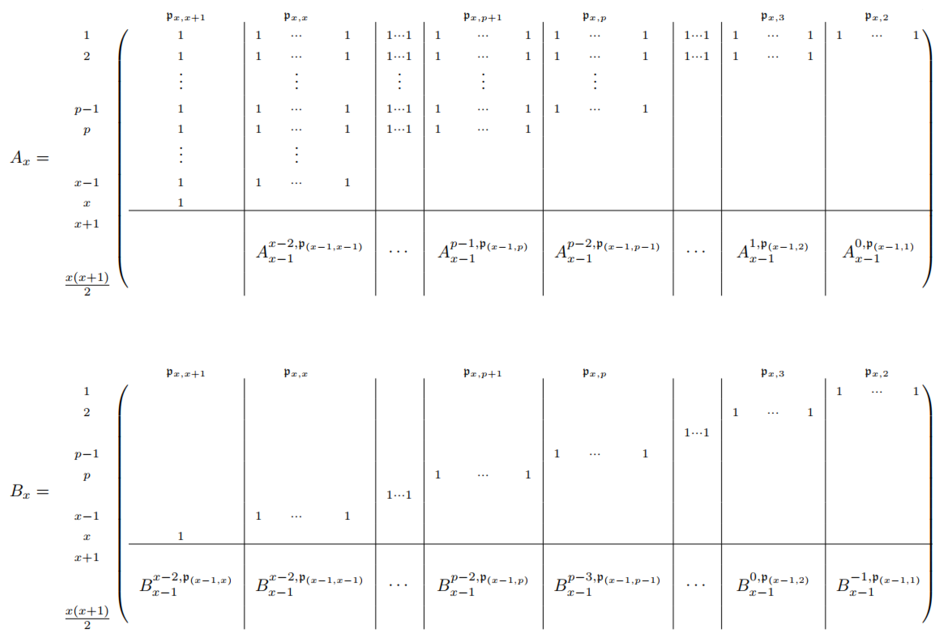
• If $p=0$ then $A_x^{0,{\mathfrak{p}}_{x,1}}$ is a matrix with ${\mathfrak{p}}_{x,1}$ columns. Then $a_i^{x,0}=v_{i,1}^{A_x}$ for $1\le i\le \frac{x(x+1)}{2}$, provided that, ${\mathfrak{p}}_{x,1}={\mathfrak{p}}_{x,2}$, $a_{i,j}^{x,0}=a_{i,j}^x$;
• If $p=1$ then $A_x^{1,{\mathfrak{p}}_{x,2}}$ is a matrix with ${\mathfrak{p}}_{x,2}$ columns, $a_{i,j}^{x,1}=a_{i,j}^x$ for $2\le i\le \frac{x(x+1)}{2}$, i.e., $a_i^{x,1}=v_{i,1}^{A_x}$ for $2\le i\le \frac{x(x+1)}{2}$, and $a_1^{x,1}=0$;
• If $2\le p\le x-1$, and $A_x^{p,{\mathfrak{p}}_{x,p+1}}$ is a matrix with ${\mathfrak{p}}_{x,p+1}$ columns. In this case, the entries of the matrix ${\left(A_x^{p,{\mathfrak{p}}_{x,p+1}}\right)}^{\prime }$ obtained from matrix $A_x^{p,{\mathfrak{p}}_{x,p+1}}$ by deleting the $p-1$th row and all columns $C_j$, ${\mathfrak{p}}_{x,p+1}\le j\le {\mathfrak{p}}_{x,p}$ equals $A_x^{p-1,{\mathfrak{p}}_{x,p}}$. Thus, the matrix $A_{x-1}^{p-2,{\mathfrak{p}}_{x-1,p-1}}$ provides entries in columns $C_j$, for which $x+1\le j\le \frac{x(x+1)}{2}$, i.e.,

  $${\displaystyle a_i^{x,p}=\sum _{q=1}^{{\mathfrak{p}}_{x,p}}{a}_{i,q}^{x,p-1}-\sum _{q=1}^{{\mathfrak{p}}_{x-1,p-1}}{a}_{i-x,q}^{x-1,p-2},}$$

  for $x+1\le i\le \frac{x(x+1)}{2}$ and $a_i^{x,p}=0$, otherwise.

The item 2 can be proved by using similar arguments as in the case 1. We are done. □

The following notation is assumed in the proof of Proposition 5.

• $a_s=1+w-(s+1)-\frac{s(s+1)-k(k+1)}{2}$;
• $b_s=s-k+w-(s+1)-(\frac{s(s+1)-k(k-1)}{2}+1)$;
• $b_x=x-k+w-(\frac{x(x+1)-k(k+1)}{2}+1)$;
• $c_s=s-k+w-(s+1)-(\frac{s(s+1)-k(k-1)}{2}+1)-(v-1)$;
• $c_x=x-k+w-(\frac{x(x+1)-k(k+1)}{2}+1)-(v-1)$;
• $d_s=1+w-\frac{(s+2)(s+1)-k(k+1)}{2}$;
• $d_x=1+w-\frac{x(x+1)-k(k+1)}{2}$;
• $e_s=s-k+w-(\frac{(s+2)(s+1)-k(k-1)}{2}+1)$;
• $f_s=s-k+w-(\frac{(s+2)(s+1)-k(k-1)}{2}+1)-(v-1)$;
• $g_s=s-k+w-\frac{(s+2)(s+1)-k(k+1)}{2}$;
• $h_s=w-\frac{(s+2)(s+1)-k(k+1)}{2}$;
• $j_s=s+1-k+w-(\frac{(s+2)(s+1)-k(k+1)}{2}+1)$;
• $k_s=v+w-(s+1)-\frac{s(s+1)-k(k+1)}{2}$.

Proposition 5.

Let $A_x$ and $B_x$ be the matrices shown in Figure 3. Then, the following identities hold.

1. 

$a_w^{x,v}={\mathfrak{p}}_{k,d_x}{\mathfrak{h}}_{x-k+1,c_x}^{b_x}$ for $0\le v\le x-1$;

2. 

$b_w^{x,v}={\mathfrak{p}}_{k-1,(d_x-1)}{\mathfrak{h}}_{(x-k+1),c_x-1}^{b_x+1}$ for $-1\le v\le x-1$,

with $\frac{n(n+1)-k(k+1)}{2}\le w\le \frac{x(x+1)-k(k-1)}{2}$ for $1\le k\le x$, and $x>1$.

Proof. 

1. If $x=2$ and $v=0$, then ${\varphi }_0\left(A_2^{0,{\mathfrak{p}}_{2,1}}\right)={\varphi }_0\left(A_2\right)$. Thus,

$$\begin{array}{c}{a}_1^{2,0}=2={\mathfrak{p}}_{2,2}{\mathfrak{h}}_{1,1}^0,\hfill \\ a_2^{2,0}=1={\mathfrak{p}}_{2,3}{\mathfrak{h}}_{1,2}^1,\hfill \\ a_3^{2,0}=1={\mathfrak{p}}_{1,2}{\mathfrak{h}}_{2,2}^1.\hfill \end{array}$$

If $v=1$ then ${\varphi }_0\left(A_2^{1,{\mathfrak{p}}_{2,2}}\right)={\varphi }_1\left(A_2\right)$, then

$$\begin{array}{c}{a}_1^{2,1}=0={\mathfrak{p}}_{2,2}{\mathfrak{h}}_{1,0}^0,\hfill \\ a_2^{2,1}=1={\mathfrak{p}}_{1,2}{\mathfrak{h}}_{1,1}^1,\hfill \\ a_3^{2,1}=1={\mathfrak{p}}_{1,2}{\mathfrak{h}}_{2,1}^1.\hfill \end{array}$$

If the result is valid for $x=s$ and $0\le v\le s$. Moreover, ${\varphi }_0\left(A_{s+1}^{0,{\mathfrak{p}}_{s+1,1}}\right)={\varphi }_0\left(A_{s+1}\right)$ if $x=s+1$ and $v=0$ (see Lemma 2). $a_w^{s+1,0}={\mathfrak{p}}_{s+1,w+v}={\mathfrak{p}}_{s+1,v+w}{\mathfrak{h}}_{1,w}^{w-1}$, $0<w<s+1$.

The rows between $s+2$ and $\frac{(s+1)(s+2)}{2}$ satisfy the following identities.

$a_w^{s+1,0}={\sum }_{v=0}^{s-1}{\mathfrak{p}}_{k,a_s}{\mathfrak{h}}_{s+1-k,c_s}^{b_s}={\mathfrak{p}}_{k,d_s}{\sum }_{v=0}^{s-1}{\mathfrak{h}}_{s+1-k,f_s}^{e_s}={\mathfrak{p}}_{k,d_s}{\mathfrak{p}}_{g_s,h_s}={\mathfrak{p}}_{k,d_s}{\mathfrak{h}}_{s+2-k,g_s+1}^{g_s}$, with $1\le k\le m$.

If $v=1$, then ${\varphi }_0\left(A_{s+1}^{1,{\mathfrak{p}}_{s+1},2}\right)={\varphi }_1\left(A_{s+1}^{0,{\mathfrak{p}}_{s,1}}\right)$. Thus, $a_1^{s+1,1}=0={\mathfrak{p}}_{s+1,2}{\mathfrak{h}}_{1,0}^0$, and

$a_w^{s+1,1}=a_w^{s+1,0}={\mathfrak{p}}_{k,d_s}{\mathfrak{h}}_{s+2-k,g_s+1}^{g_s}={\mathfrak{p}}_{k,d_s}{\mathfrak{h}}_{s+2-k,g_s}^{g_s}$. For $\frac{(s+2)(s+1)-k(k+1)}{2}<w\le \frac{(s+2)(s+1)-k(k-1)}{2}$ with $w\ne 1$, and $1\le k\le s+1$.

If the proposition holds for $v=p-1<s$. Therefore, it holds that ${\varphi }_0\left(A_{s+1}^{p,{\mathfrak{p}}_{s+1,p+1}}\right)={\varphi }_p\left(A_{s+1}^{p-1,{\mathfrak{p}}_{s+1,p}}\right)+{\phi }_{s+1}\left(A_s^{p-2,{\mathfrak{p}}_{(s,p-1)}}\right)$ if $v=p$ (see Lemma 2).

$a_w^{s+1,p}=0={\mathfrak{p}}_{s+1,1+w}{\mathfrak{h}}_{1,w-p}^{w-1},$ for $1\le w\le p$.

$a_w^{s+1,p}=a_w^{s+1,p-1}={\mathfrak{p}}_{s+1,1+u}{\mathfrak{h}}_{1,w+1-p}^{w-1}={\mathfrak{p}}_{s+1,1+w}{\mathfrak{h}}_{1,w-p}^{w-1}$, for $p+1\le w\le s+1.$

$a_w^{s+1,p}={\mathfrak{p}}_{k,d_s}{\mathfrak{h}}_{s+2-k,j_s-(p-2)}^{j_s}-{\mathfrak{p}}_{k,l_s}{t}_{b_s+k,b_s+k-(p-3)}^{s+1-k}$, for $w\ge s+1$.

Proposition 1 implies that

$a_w^{s+1,p}={\mathfrak{p}}_{k,k_s}{\mathfrak{h}}_{s+2-k,j_s-(p-1)}^{j_s},$ for $1\le k\le s$.

The proof of case 2 requires similar arguments as those exposed in case 1. We are done. □

The following map $\delta :\mathbb{N}\to \{1,2\}$ such that

$$\delta \left(x\right)=\left\{\begin{array}{cc}1,\hfill & \mathrm{if} x\ne 2,\hfill \\ 2,\hfill & \mathrm{if} x=2.\hfill \end{array}\right.$$

is used to give dimension formulas for Catalan–Brauer algebras ${\Gamma }^x$ and their centers.

Theorem 2.

Let ${\Lambda }_{{\Gamma }^x}$ be a Catalan–Brauer configuration algebra. Then

1. 

${\displaystyle \frac{{\dim }_{\mathbb{F}}{\Lambda }_{{\Gamma }^x}}{2}=\frac{1}{n+1}\left(\genfrac{}{}{0pt}{}{2x}{x}\right)+\delta \left(x\right)+\sum _{u=1}^{\frac{x(x+1)}{2}}(t_{(a_u^{x,0}-1)}+t_{(b_u^{x,0}-1)})}$.

2. 

${\dim }_{\mathbb{F}}Z\left({\Lambda }_{{\Gamma }^x}\right)=1+2\delta \left(x\right)+\frac{1}{x+1}\left(\genfrac{}{}{0pt}{}{2x}{x}\right).$

where, $x>0$ and $t_i$ denotes the ith triangular number.

Proof. 

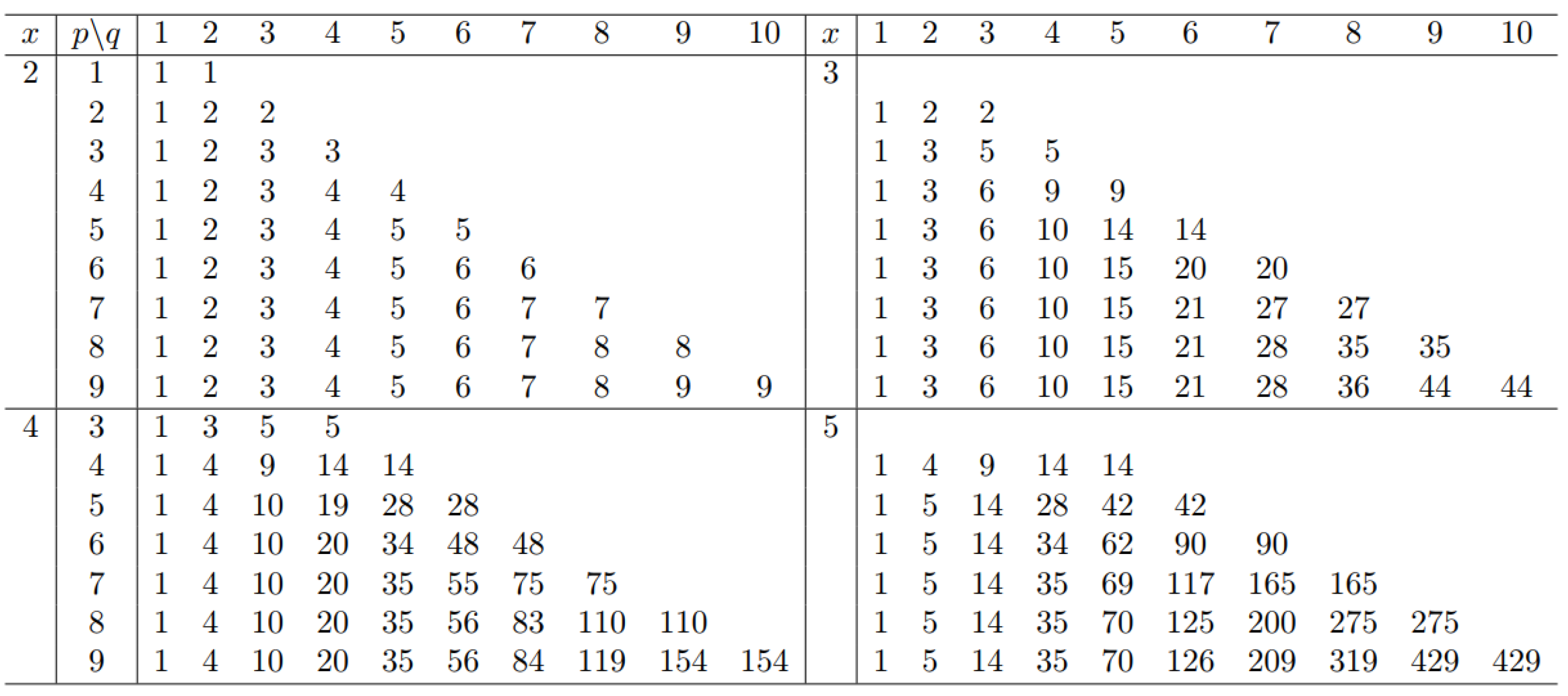
• Firstly, we note that the number of vertices in the Brauer quiver $Q_{{\Gamma }_x}$ is given by the xth Catalan number $C_x=\frac{1}{x+1}\left(\genfrac{}{}{0pt}{}{2x}{x}\right)$. Secondly, we note that $val\left({\mathfrak{a}}_{x_1}^{x_2}\right)$ (resp. $val\left({\mathfrak{b}}_{n_1}^{n_2}\right)$) is given by $a_{m_a}^{x,0}$, $m_a=x{x}_1+x_2-\frac{x_1(x_1+1)}{2}$ (resp. $b_{m_b}^{x,0}$, $m_b=x{x}_1+x_2-\frac{x_1(x_1+1)}{2}$). As a consequence of Proposition 5, we have that $a_x^{x,0}=1=b_x^{x,0}$ for any x. In particular, for $x=2$, it holds that $a_2^{0,1}=b_2^{0,1}=1$.
• $\#Loops\left(Q_{{\Lambda }_{{\Gamma }^x}}\right)=\left|{\mathcal{C}}_{{\Lambda }_{{\Gamma }^x}}\right|$ (see identity (8)).

□

As an example, the following are the dimensions associated with the Brauer configuration (20). We note that for $x=2$, it holds that $C_2=2$, $a_1^{2,0}=2=b_3^{2,0}$, and $a_2^{2,0}=a_3^{2,0}=b_1^{2,0}=b_2^{2,0}=1$. Thus

$$\begin{array}{cc}\hfill {\dim }_{\mathbb{F}}{\Lambda }_{{\Gamma }^2}& =2(C_2+\delta \left(2\right))+12-8\hfill \\ & =2(2+2)+4=12,\hfill \end{array}$$

and

$${\dim }_{\mathbb{F}}Z\left({\Lambda }_{{\Gamma }^2}\right)=1+2\delta \left(2\right)+C_2=7.$$

4. Concluding Remarks

Catalan–Brauer configuration algebras (CBCAs) is a way to relate Catalan combinatorics with the BCAs theory. Dimension formulas of such CBCAs and their centers can be obtained by using entries of the Catalan triangle. The procedure interprets such entries as numbers of some novel integer sequences ${\mathfrak{h}}_{x,j}^i$ dealing with binomial numbers.

It is an interesting task for the future to investigate additional relationships between sequences ${\mathfrak{h}}_{x,j}^i$ and different Catalan objects.

References

- Stanley, R.P. Enumerative Combinatorics; Cambridge University Press: Cambridge, UK, 1999; Volume 2. [Google Scholar]
- Caldero, P.; Chapoton, F.; Schiffler, R. Quivers with relations arising from clusters (n case). Trans. Am. Math. Soc. 2006, 358, 1347–1364. [Google Scholar] [CrossRef] [Green Version]
- Cañadas, A.M.; Gaviria, I.D.M.; Espinosa, P.F.F.; Rios, G.B. Coxeter’s frieze patterns arising from Dyck paths. Ric. Mat. 2021. [Google Scholar] [CrossRef]
- Green, E.L.; Schroll, S. Brauer configuration algebras: A generalization of Brauer graph algebras. Bull. Sci. Math. 2017, 121, 539–572. [Google Scholar] [CrossRef] [Green Version]
- Espinosa, P.F.F. Categorification of Some Integer Sequences and Its Applications. Ph.D. Thesis, Universidad Nacional de Colombia, Bogotá, Colombia, 2021. [Google Scholar]
- Cañadas, A.M.; Gaviria, I.D.M.; Vega, J.D.C. Relationships between the Chicken McNugget Problem, Mutations of Brauer Configuration Algebras and the Advanced Encryption Standard. Mathematics 2021, 9, 1937. [Google Scholar] [CrossRef]
- Sapir, M.V. Combinatorial Algebra: Syntax and Semantics; Guba, V.S., Volkov, M.V., Contributor; Springer Monographs in Mathematics; Springer: Cham, Switzerland, 2014; 355p, ISBN 978-3-319-08030-7. [Google Scholar]
- Ufnarovskij, V.A. Combinatorial and asymptotic methods in algebra. Algebra VI. Encycl. Math. Sci. 1990, 57, 1–196, Translation from Itogi Nauki Tekh. Ser. Sovrem. Probl. Mat. Fundam. Napravleniya 1990, 57, 5–177. [Google Scholar]
- Belov, A.Y.; Borisenko, V.V.; Latyshev, V.N. Monomial algebras. J. Math. Sci. (N. Y.) 1997, 87, 3463–3575. [Google Scholar] [CrossRef]
- Lee, K.H.; Oh, S.J. Catalan triangle numbers and binomial coefficients. Contemp. Math. Am. Math. Soc. 2018, 713, 165–185. [Google Scholar]
- Schroll, S. Brauer Graph Algebras. In Homological Methods, Representation Theory, and Cluster Algebras, CRM Short Courses; Assem, I., Trepode, S., Eds.; Springer: Cham, Switzerland, 2018; pp. 177–223. [Google Scholar]
- Sierra, A. The dimension of the center of a Brauer configuration algebra. J. Algebra 2018, 510, 289–318. [Google Scholar] [CrossRef]
Publisher’s Note: MDPI stays neutral with regard to jurisdictional claims in published maps and institutional affiliations. |
© 2022 by the authors. Licensee MDPI, Basel, Switzerland. This article is an open access article distributed under the terms and conditions of the Creative Commons Attribution (CC BY) license (https://creativecommons.org/licenses/by/4.0/).
Share and Cite
Cañadas, A.M.; Rios, G.B.; Gaviria, I.D.M. Brauer Configuration Algebras Arising from Dyck Paths. Mathematics 2022, 10, 1378. https://doi.org/10.3390/math10091378
Cañadas AM, Rios GB, Gaviria IDM. Brauer Configuration Algebras Arising from Dyck Paths. Mathematics. 2022; 10(9):1378. https://doi.org/10.3390/math10091378
Chicago/Turabian StyleCañadas, Agustín Moreno, Gabriel Bravo Rios, and Isaías David Marín Gaviria. 2022. "Brauer Configuration Algebras Arising from Dyck Paths" Mathematics 10, no. 9: 1378. https://doi.org/10.3390/math10091378