A Comparative Study of SSA-BPNN, SSA-ENN, and SSA-SVR Models for Predicting the Thickness of an Excavation Damaged Zone around the Roadway in Rock

Abstract

Due to the disturbance effect of excavation, the original stress is redistributed, resulting in an excavation damaged zone around the roadway. It is significant to predict the thickness of an excavation damaged zone because it directly affects the stability of roadways. This study used a sparrow search algorithm to improve a backpropagation neural network, and an Elman neural network and support vector regression models to predict the thickness of an excavation damaged zone. Firstly, 209 cases with four indicators were collected from 34 mines. Then, the sparrow search algorithm was used to optimize the parameters of the backpropagation neural network, Elman neural network, and support vector regression models. According to the optimal parameters, these three predictive models were established based on the training set (80% of the data). Finally, the test set (20% of the data) was used to verify the reliability of each model. The mean absolute error, coefficient of determination, Nash–Sutcliffe efficiency coefficient, mean absolute percentage error, Theil’s U value, root-mean-square error, and the sum of squares error were used to evaluate the predictive performance. The results showed that the sparrow search algorithm improved the predictive performance of the traditional backpropagation neural network, Elman neural network, and support vector regression models, and the sparrow search algorithm–backpropagation neural network model had the best comprehensive prediction performance. The mean absolute error, coefficient of determination, Nash–Sutcliffe efficiency coefficient, mean absolute percentage error, Theil’s U value, root-mean-square error, and sum of squares error of the sparrow search algorithm–backpropagation neural network model were 0.1246, 0.9277, −1.2331, 8.4127%, 0.0084, 0.1636, and 1.1241, respectively. The proposed model could provide a reliable reference for the thickness prediction of an excavation damaged zone, and was helpful in the risk management of roadway stability.

1. Introduction

After the excavation of roadway, the initial stress in the surrounding rock mass is redistributed. When the stress is greater than the strength of the surrounding rock, the rock mass will be damaged. Then, a ringlike broken zone can be formed around the excavated space; this is called the excavation damaged zone (EDZ) [1,2]. The thickness of the EDZ can not only be used to judge the stability of the roadway, but can also be adopted in the support design [3,4,5]. In addition, due to the weakening in the rock strength, an EDZ can also be utilized for nonexplosive continuous mining in deep hard-rock mines [6]. Therefore, predicting the thickness of the EDZ around a roadway is significant.

Since the concept of the EDZ was proposed, many scholars have conducted plenty of research to determine its size or thickness. These methods can be mainly summarized as the onsite measurement technique, the numerical simulation method, the empirical formula, and the machine-learning (ML) algorithm. Among them, the onsite measurement technique is the most direct method to determine the thickness of an EDZ, and includes digital panoramic drilling camera technology [7], ground-penetrating radar [8], ultrasonic detection technology [9], the borehole imaging method [10], the complex resistivity method [11], and microseismic monitoring [12,13]. Although the results of these measurements are accurate, the operation is complicated and vulnerable to the site conditions. With the rapid development of rock mechanics and computers, numerical-simulation methods became popular to determine the thickness of an EDZ. Liu et al. [14] used the ANSYS software to analyze the influencing factors and distribution law of an EDZ around a rectangular roadway. Sun et al. [15] studied the formation mechanism of a butterfly-shaped EDZ by combining the force and elastic wave theory, and then used Midas/GTS-FLAC3D simulation technology to determine the range of the EDZ. Perras et al. [16] used the finite element method in the Phase2 software to determine the thickness of an EDZ. Wan et al. [17] used 3DEC to determine the thickness of an EDZ, and the simulation results were consistent with the measured values. Although a numerical simulation is low-cost and convenient to operate, many assumptions exist in the simulation process that lead to idealized results and affect the accuracy. According to field-engineering experience and theoretical analysis, some empirical formulas were proposed to calculate the thickness of an EDZ. Yan [18] proposed an empirical formula for the thickness prediction of an EDZ based on the wave velocity of the rock and rock mass. Wang [19] combined the elastoplastic theory and measured data to determine the range of the EDZ in the Chazhen Tunnel. Chen et al. [20] deduced the radius of an EDZ based on the Hoek–Brown criterion and elastoplastic solution of a circular hole. Based on similar simulation tests and field experience, Dong [4] proposed a relationship between the stress and the rock strength to calculate the thickness of an EDZ. Zhao [21] derived the quantitative relationship between the thickness of an EDZ and its influencing factors based on a dimensional-analysis method. In addition, the zonal disintegration phenomenon, which indicates the alternation of fractured and intact zones, appears in deep roadways. Shemyakin [22] proposed the concept of zonal disintegration and deduced the empirical formula for the thickness of the discontinuous zone. After Myasnikov [23] proposed a non-Euclidean continuum model to describe the stress-field distribution, some scholars [24,25,26] used that non-Euclidean model to investigate the zonal disintegration phenomenon in a surrounding rock mass, and obtained the corresponding formulas. Although an empirical formula is easy to understand, it ignores the effects of joints and mining. Currently, there is no universally accepted empirical formula for predicting the thickness of an EDZ.

Considering ML can well deal with nonlinear and complex problems [27,28], it shows great potential to predict the thickness of an EDZ. Asadi et al. [29] used artificial neural networks in the thickness prediction of an EDZ. Zhou [30] verified that the support vector machine (SVM) could reliably estimate the range of an EDZ. In addition, some scholars adopted intelligent optimization techniques to improve traditional ML algorithms for the determination of an EDZ’s thickness. For example, Hu [31] used a layered fish school to improve the SVM; Ma [32] combined the particle-swarm algorithm (PSO) and the least-squares support vector machine; Yu [33] integrated PSO and a Gaussian process model; and Liu [34] employed the wavelet-relevance vector machine. In addition, ML is being increasingly used in other civil engineering fields, and achieves an excellent prediction performance [35,36,37]. For example, Mangalathu et al. [38] used ML to classify the building damage caused by earthquakes; Ruggieri et al. [39] adopted ML to analyze the vulnerability of existing buildings. ML can not only obtain reliable prediction results, but can also save time and economic costs. However, numerous EDZ cases are needed to improve its credibility.

After comparing it with other types of approaches, the ML method was preferentially chosen to predict the thickness of an EDZ. An important reason is that it has strong self-learning and adaptive capabilities based on big data and can find implicit relationships between indicators. Nevertheless, it is essential to determine the favorable parameters of ML, because they directly affect its predictive performance [40]. The sparrow search algorithm (SSA) proposed by Xue [41] in 2020 is an efficient swarm-intelligence optimization algorithm. Compared with other optimization algorithms, the SSA has a higher search efficiency and a simpler operation. SSA considers all possible situations of a sparrow population, so that the sparrows in the population are close to the global optimal value, and converge [42]. At the same time, SSA has a high convergence speed, a good stability, a strong global search ability, and few parameters. In addition, backpropagation neural network (BPNN), Elman neural network (ENN), and support vector regression (SVR) models have shown extraordinary capabilities in solving prediction problems, and have been widely used in various engineering fields [43,44,45]. Therefore, using SSA to optimize the parameters of BPNN, ENN, and SVR models is more competitive.

The goal of this study was to use SSA-BPNN, SSA-ENN, and SSA-SVR models to predict the thickness of an EDZ. Firstly, an EDZ database including 209 cases was established. Secondly, SSA-BPNN, SSA-ENN, and SSA-SVR models were proposed for the thickness prediction of an EDZ. Thirdly, seven indexes were used to evaluate the performance of each model. Finally, all models were compared and analyzed, and the best model was determined.

2. Data Collection

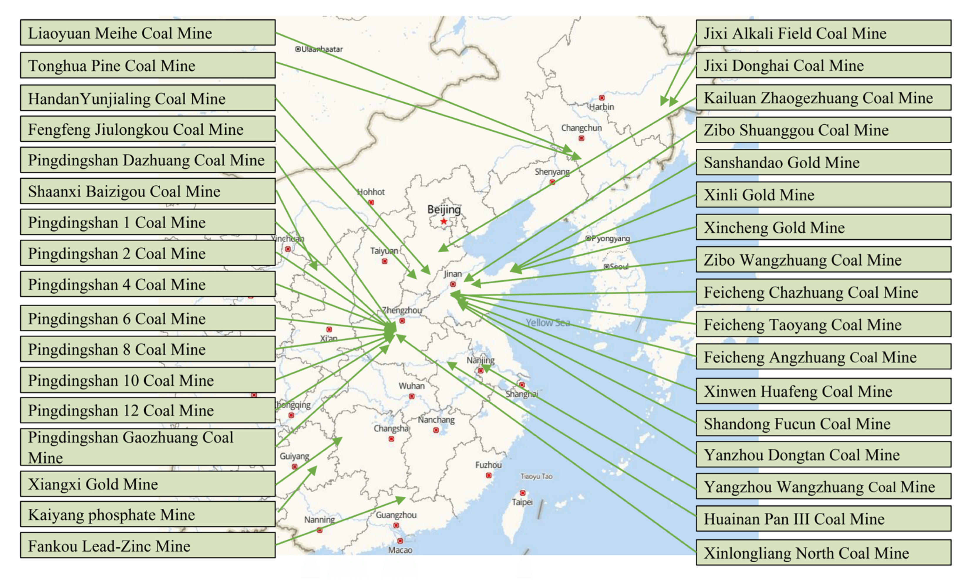
To establish a reliable predictive model, a total of 209 cases from 34 mines were collected [46,47,48,49,50]. The locations of these mines are shown in Figure 1. It can be seen that the types of these mines were different, and included coal mines, gold mines, phosphate mines, and lead–zinc mines. In addition, these mines were in different regions, which indicated that the collected dataset was complex to some extent.

The dataset statistics of each indicator are shown in

Table 1. Statistics for each indicator.

Indicator	Max	Min	Mean	Standard Deviation
$A_1$ (m)	1159.00	97.00	499.20	242.94
$A_2$ (m)	10.00	2.40	3.71	1.13
$A_3$ (MPa)	158.83	7.50	30.80	31.12
$A_4$	5.00	1.00	2.89	1.15
$A_5$ (m)	3.45	0.30	1.56	0.61

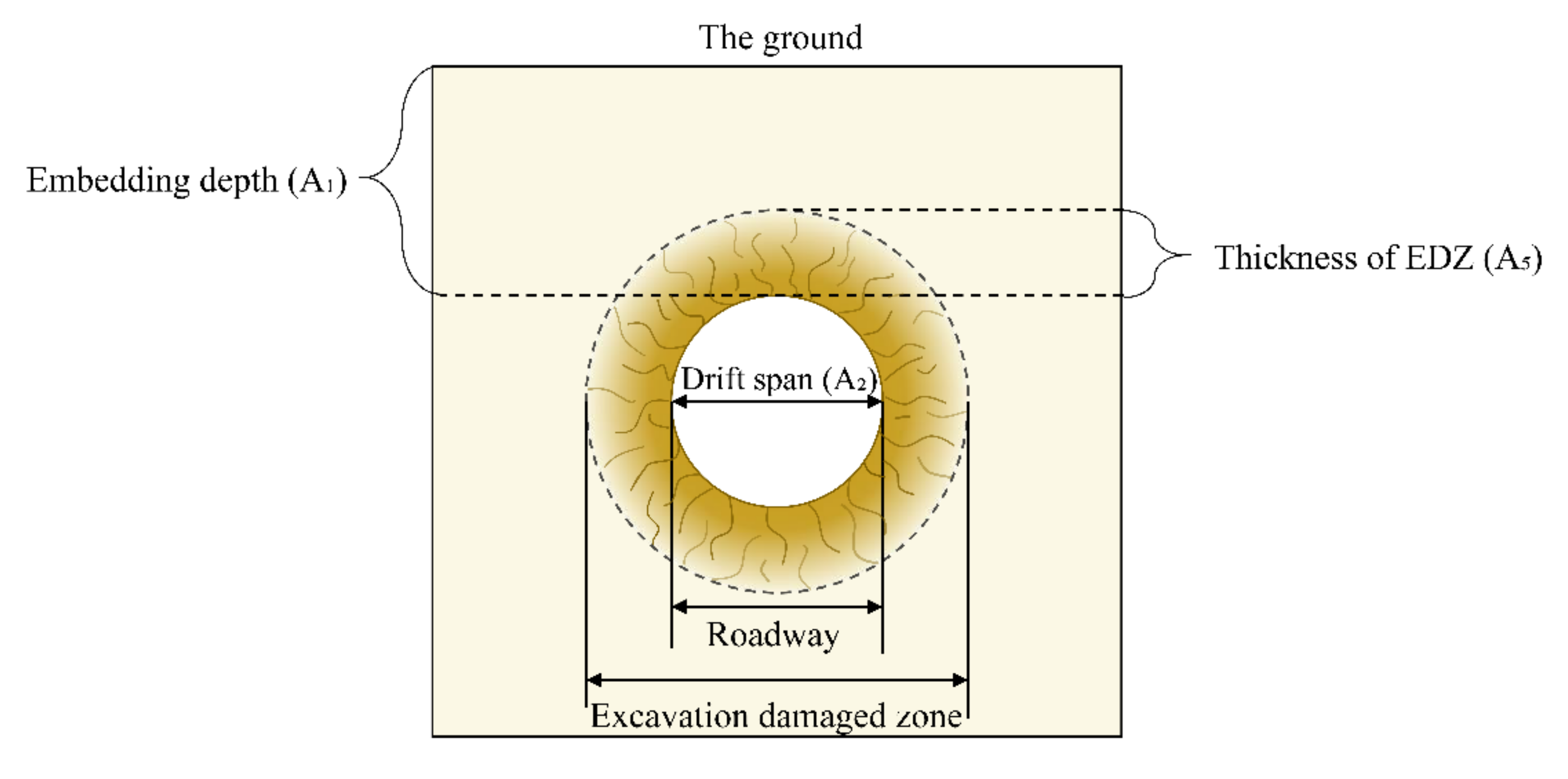
, where $A_1$ indicates the embedding depth, $A_2$ indicates the drift span, $A_3$ indicates the surrounding rock strength, $A_4$ indicates the joint index, and $A_5$ indicates the EDZ thickness. The complete data can be found in Appendix A 

Table A1. Database of EDZ cases.

Samples	A1/m	A2/m	A3/MPa	A4	A5/m
1	800.00	4.00	48.00	3.00	1.62
2	800.00	3.60	67.00	4.00	2.14
3	650.00	6.00	16.80	5.00	3.45
4	220.00	3.40	21.30	4.00	1.31
5	876.40	3.40	13.80	3.00	1.41
6	321.00	3.00	13.30	1.00	2.41
7	420.00	3.20	9.10	4.00	1.40
8	800.00	3.60	70.60	3.00	1.84
9	340.00	3.40	18.80	1.00	1.52
10	315.00	2.80	11.20	1.00	1.77
11	740.00	3.30	32.42	3.00	2.00
12	1154.00	4.20	15.94	2.00	1.53
13	720.00	4.80	102.40	2.00	1.10
14	125.00	2.80	13.30	2.00	0.70
15	680.00	3.30	30.49	3.00	2.10
16	199.00	3.60	10.73	3.00	1.30
17	252.00	5.20	15.08	4.00	2.65
18	660.00	3.60	21.96	5.00	2.20
19	140.00	3.60	13.40	2.00	0.50
20	342.50	3.20	15.94	2.00	0.39
21	280.00	2.80	12.70	2.00	0.80
22	665.00	3.60	10.90	2.00	2.94
23	510.00	8.00	54.87	3.00	1.40
24	350.00	3.20	10.50	1.00	1.93
25	689.00	3.00	15.10	4.00	1.80
26	321.00	2.60	13.30	3.00	1.10
27	615.00	3.60	25.64	3.00	1.50
28	510.00	4.00	64.54	2.00	1.10
29	740.00	4.00	22.70	5.00	2.25
30	249.00	3.20	16.80	1.00	2.46
31	961.00	4.00	12.76	3.00	1.57
32	362.00	2.60	62.40	2.00	0.60
33	680.00	3.80	25.64	5.00	2.35
34	180.00	2.80	110.20	1.00	0.89
35	342.50	3.20	13.80	3.00	0.55
36	403.00	2.90	12.60	1.00	1.90
37	150.00	3.60	14.60	2.00	0.60
38	510.00	3.70	12.60	4.00	1.40
39	470.00	3.60	9.10	2.00	3.26
40	876.40	3.60	12.76	3.00	1.48
41	660.00	4.40	12.50	5.00	2.20
42	610.00	3.00	34.00	3.00	1.35
43	869.00	4.00	67.00	4.00	1.78
44	340.00	3.40	18.80	3.00	1.30
45	450.00	3.00	11.20	1.00	2.11
46	350.00	3.20	10.50	3.00	1.20
47	680.00	4.20	47.00	3.00	1.40
48	400.00	5.32	21.71	3.00	1.62
49	740.00	2.60	32.42	2.00	1.50
50	520.00	3.80	11.90	2.00	2.59
51	480.00	3.00	10.35	3.00	1.20
52	470.00	4.00	10.10	2.00	2.97
53	300.00	4.50	20.00	3.00	1.50
54	300.00	4.50	20.00	4.00	1.60
55	340.00	3.00	73.60	1.00	0.99
56	961.00	3.60	15.94	2.00	1.35
57	850.00	3.80	48.00	1.00	1.04
58	690.00	4.60	47.00	3.00	1.50
59	1154.00	4.20	13.80	3.00	1.69
60	178.00	2.60	23.80	3.00	1.20
61	710.00	6.00	16.80	4.00	3.20
62	125.00	2.80	13.30	1.00	1.91
63	630.00	4.80	52.45	2.00	1.20
64	310.00	3.20	28.00	1.00	1.33
65	800.00	5.10	28.22	4.00	2.43
66	218.00	3.89	38.11	3.00	0.70
67	837.00	3.80	70.00	1.00	0.67
68	525.00	3.20	15.80	4.00	1.60
69	220.00	3.40	7.80	4.00	1.50
70	97.00	2.60	11.20	3.00	1.20
71	97.00	2.60	11.20	1.00	1.70
72	125.00	2.80	13.30	3.00	1.30
73	700.00	3.60	16.80	5.00	2.55
74	450.00	3.40	9.10	2.00	2.36
75	685.00	3.60	25.64	3.00	1.78
76	1154.00	4.20	12.76	3.00	1.77
77	961.00	4.00	10.00	5.00	2.46
78	700.00	3.80	25.64	3.00	1.78
79	460.00	3.20	101.60	1.00	0.99
80	410.00	3.00	26.78	3.00	1.00
81	665.00	3.60	10.90	4.00	1.70
82	400.00	5.32	15.30	3.00	1.90
83	876.40	3.60	10.00	5.00	2.34
84	700.00	3.60	48.00	3.00	1.40
85	125.00	3.40	13.30	3.00	1.00
86	705.00	3.80	16.80	5.00	2.85
87	316.00	8.00	78.43	4.00	1.90
88	392.00	2.80	14.50	2.00	0.80
89	340.00	3.20	32.20	2.00	0.70
90	357.00	3.20	10.50	3.00	1.10
91	665.00	4.40	10.90	4.00	1.70
92	293.00	3.50	11.90	1.00	1.93
93	329.67	2.40	44.72	3.00	0.70
94	362.00	2.60	58.00	2.00	0.80
95	869.00	3.80	70.00	3.00	1.21
96	480.00	3.00	15.00	3.00	1.00
97	620.00	3.60	21.96	5.00	2.12
98	410.00	3.20	13.30	1.00	2.32
99	244.00	3.40	11.20	3.00	1.00
100	690.00	4.80	9.20	4.00	2.10
101	420.00	3.20	9.10	1.00	2.85
102	293.00	3.50	11.90	3.00	1.10
103	660.00	3.60	21.96	4.00	2.20
104	675.00	3.80	25.64	4.00	2.10
105	296.00	3.40	22.40	3.00	1.20
106	296.00	3.40	22.40	1.00	1.67
107	236.00	3.00	14.30	1.00	2.00
108	410.00	3.60	13.30	4.00	1.40
109	313.00	10.00	38.00	3.00	1.76
110	340.00	3.20	32.20	1.00	1.31
111	252.00	5.20	17.23	4.00	2.41
112	450.00	3.60	13.30	2.00	2.58
113	520.00	3.80	11.90	4.00	1.70
114	296.00	3.40	22.40	4.00	1.40
115	720.00	4.80	86.30	2.00	1.20
116	268.00	3.40	11.96	4.00	1.40
117	490.00	3.70	12.50	4.00	1.50
118	321.00	3.00	13.30	3.00	1.10
119	450.00	3.60	13.30	4.00	1.60
120	410.00	3.20	13.30	4.00	1.40
121	720.00	10.00	102.40	2.00	1.20
122	192.70	2.40	35.83	4.00	0.85
123	400.00	5.32	10.61	3.00	2.10
124	868.00	3.80	60.00	1.00	0.98
125	872.00	4.00	48.00	2.00	1.49
126	610.00	3.60	22.40	4.00	1.75
127	420.00	3.20	9.10	4.00	1.70
128	510.00	8.00	54.87	3.00	1.50
129	345.00	3.00	65.00	2.00	0.70
130	200.00	3.00	15.12	4.00	0.90
131	510.00	4.00	64.54	2.00	1.20
132	342.50	3.40	12.76	3.00	0.62
133	470.00	3.60	9.10	5.00	2.10
134	1056.00	4.00	15.94	2.00	1.44
135	403.00	2.90	12.60	3.00	1.30
136	876.40	3.40	15.94	2.00	1.26
137	467.00	3.40	10.10	4.00	1.80
138	322.00	4.40	14.30	4.00	1.50
139	208.00	3.40	42.41	2.00	0.38
140	268.00	3.40	11.96	1.00	2.05
141	249.00	3.40	16.80	3.00	1.00
142	178.00	2.60	23.80	1.00	1.12
143	520.00	4.20	25.43	3.00	1.30
144	690.00	4.80	32.00	2.00	1.70
145	1159.00	4.50	13.80	4.00	2.21
146	460.00	3.20	101.60	1.00	0.40
147	310.00	3.20	28.00	3.00	0.80
148	780.00	3.00	70.60	1.00	0.65
149	450.00	3.40	9.10	5.00	2.00
150	180.00	2.80	110.20	1.00	0.30
151	550.00	3.40	12.50	5.00	2.10
152	467.00	3.40	10.10	2.00	2.31
153	231.00	3.00	18.30	2.00	0.70
154	340.00	3.20	19.80	3.00	1.30
155	685.00	3.20	52.00	2.00	1.20
156	305.00	3.20	10.10	4.00	1.30
157	321.00	2.60	9.20	3.00	1.20
158	420.00	3.60	14.30	1.00	1.98
159	670.00	3.60	16.80	5.00	2.35
160	370.00	3.50	10.50	1.00	2.00
161	236.00	3.00	14.30	3.00	1.20
162	510.00	3.20	12.60	4.00	1.60
163	1154.00	4.50	10.00	5.00	2.73
164	630.00	4.80	48.97	3.00	1.42
165	520.00	4.20	63.54	3.00	1.10
166	373.00	2.50	14.60	2.00	0.90
167	305.00	3.20	10.10	1.00	1.98
168	384.00	3.50	8.50	3.00	1.20
169	500.00	3.00	38.50	4.00	1.77
170	640.00	3.60	25.64	4.00	1.98
171	420.00	3.60	14.30	3.00	1.10
172	480.00	2.80	10.00	3.00	1.10
173	343.00	3.20	32.20	2.00	0.70
174	325.07	2.40	17.15	5.00	2.20
175	213.00	10.00	48.00	2.00	1.40
176	480.00	3.80	64.50	3.00	1.00
177	1056.00	4.00	10.00	5.00	2.60
178	348.00	3.20	7.50	3.00	1.20
179	600.00	3.60	16.80	5.00	2.25
180	362.00	2.60	62.40	1.00	0.94
181	510.00	3.70	12.60	1.00	2.47
182	310.00	2.80	13.80	3.00	1.20
183	465.00	4.00	9.50	4.00	1.60
184	961.00	3.60	13.80	3.00	1.50
185	322.00	4.40	14.30	2.00	2.88
186	315.00	2.80	11.20	3.00	1.10
187	370.00	3.50	10.50	3.00	1.00
188	630.00	4.00	21.96	5.00	2.60
189	410.00	3.20	13.30	3.00	1.10
190	1056.00	4.00	12.76	3.00	1.67
191	246.00	3.20	38.20	3.00	0.80
192	435.00	2.80	15.20	3.00	1.20
193	690.00	4.20	32.00	2.00	1.58
194	276.00	2.60	15.90	2.00	0.80
195	428.00	3.60	16.50	3.00	1.20
196	680.00	2.60	22.70	5.00	2.20
197	420.00	3.70	9.10	4.00	1.40
198	400.00	5.32	66.31	4.00	1.32
199	740.00	3.80	38.00	4.00	2.00
200	680.00	3.30	22.70	5.00	2.35
201	450.00	3.00	11.20	3.00	1.20
202	292.00	3.40	12.50	4.00	1.40
203	1056.00	4.00	13.80	3.00	1.60
204	676.00	4.00	35.00	3.00	1.60
205	680.00	2.60	36.14	3.00	1.90
206	470.00	4.00	10.10	5.00	2.20
207	264.00	3.20	11.20	3.00	1.10
208	249.00	3.20	16.80	3.00	1.00
209	340.00	3.00	73.60	2.00	0.80

. It should be noted that EDZ indicates the ruptured zone around the roadway, but not the zonal disintegration. For a better understanding, the structure of an EDZ and some indicators are illustrated in Figure 2. The meaning of these indicators is indicated in

Table 2. Meanings of these indicators.

Indicator	Meaning
$A_1$ (m)	Indicates the depth of the roadway from the ground.
$A_2$ (m)	Indicates the width of the roadway.
$A_3$ (MPa)	Indicates the uniaxial compressive strength of the surrounding rock.
$A_4$	Indicates the development degree of joints in the surrounding rock.

.

Each sample contained four indicators and the thickness of the EDZ. The thickness of an EDZ is affected by many factors, such as the strength of surrounding rock mass, in situ stress, size and shape of the roadway, excavation method, time effect, and other environmental factors. First of all, the strength of the surrounding rock mass reflects the ability of the rock mass to resist damage, and is inversely proportional to the thickness of EDZ. Therefore, the indicators $A_3$ and $A_4$ were selected. Second, considering that the thickness of an EDZ is proportional to the in situ stress around the roadway, the indicator $A_1$ was chosen. Third, because different roadway sizes have diverse influences on an EDZ, $A_2$ was used as an indicator. Fourth, since the thickness of the EDZ used in this study was a stable value, the time effect could be ignored. When considering the influence of other factors, such as temperature, groundwater, and excavation method, they were deemed too complicated to quantify, and were not considered in this study.

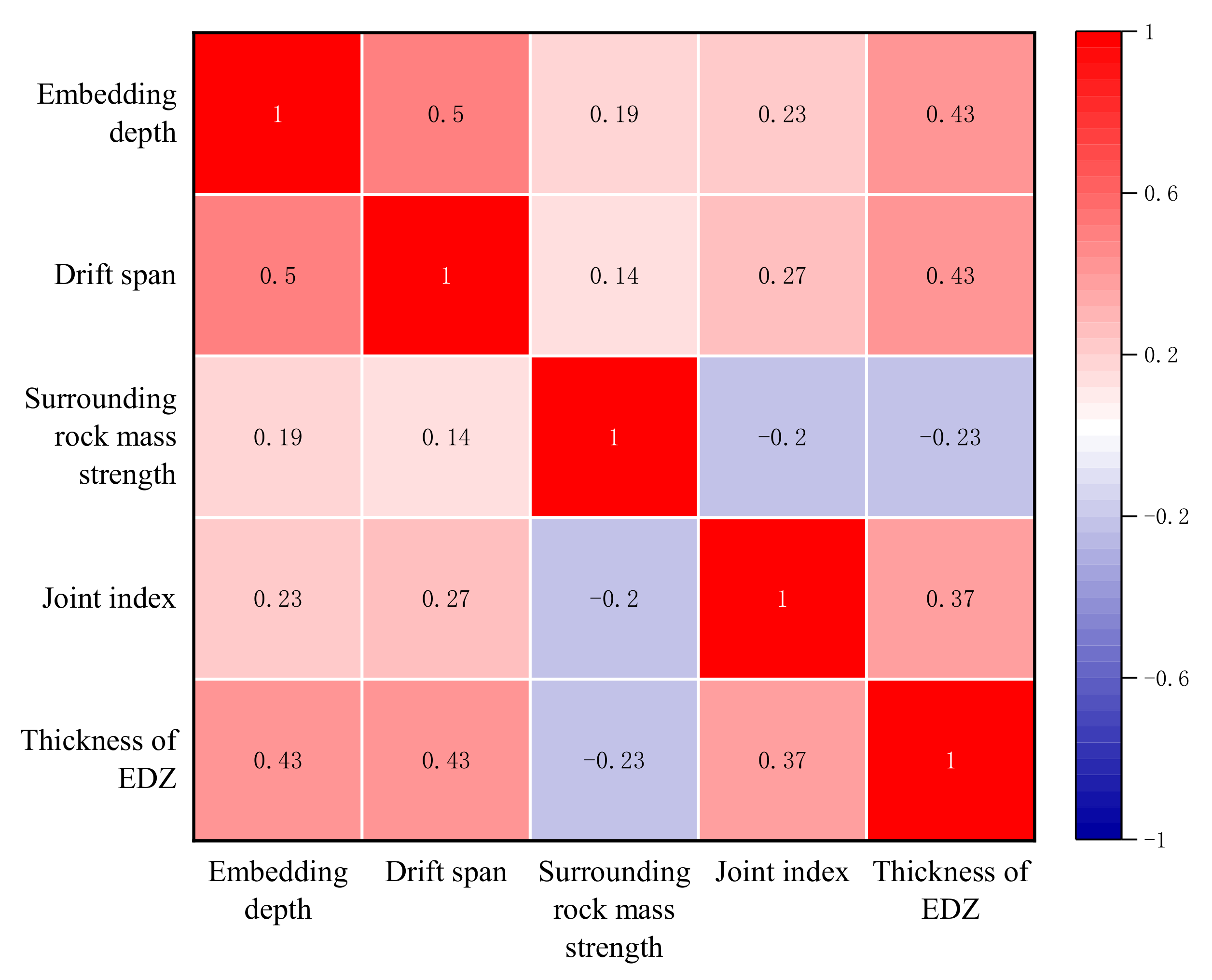
To quantitatively describe the correlation between indicators and the thickness of an EDZ, the Pearson correlation coefficient was calculated, as shown in Figure 3. In this figure, red represents a positive correlation, blue represents a negative correlation, and the depth of color indicates the strength of correlation. It can be seen that the thickness of an EDZ and these four indicators had different correlation degrees, which showed that these indicators were relatively independent. Therefore, these four indicators were used as the input variables.

The advantages of these selected indicators can be summarized as: (1) they could reflect the main factors affecting the formation of an EDZ; (2) their values were easy to obtain; and (3) the information described by these indicators was independent.

3. Methodology

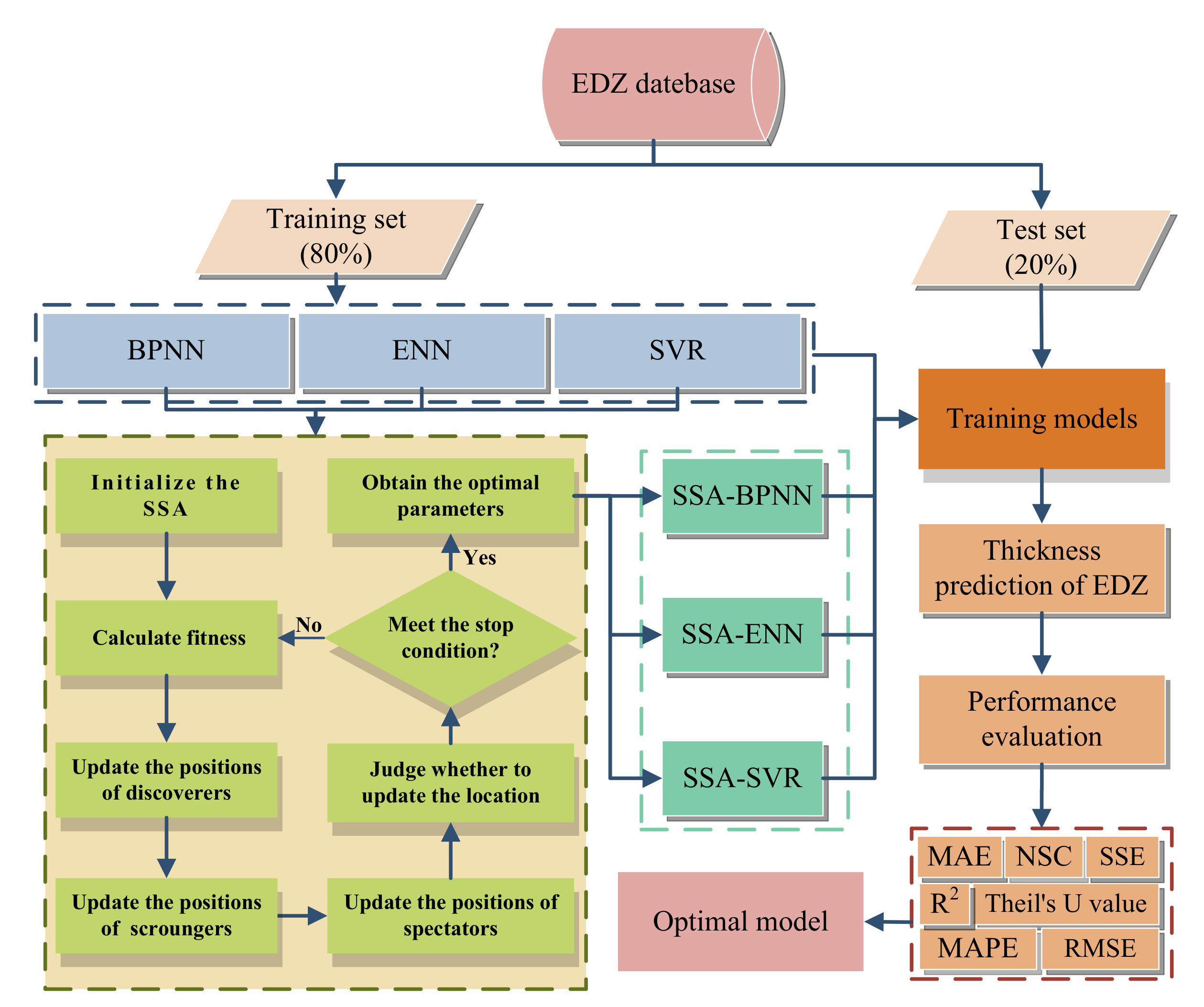
The structure of the proposed methodology is shown in Figure 4. Firstly, the original data were randomly divided into a training set (80%) and test set (20%). Secondly, the SSA was used to optimize the parameters of the BPNN, ENN and SVR models. Thirdly, the training set was adopted to train the optimized model. Fourthly, the test set was employed to analyze the accuracy of each model, and seven indexes, including the mean absolute error (MAE), coefficient of determination (R²), Nash–Sutcliffe efficiency coefficient (NSC), mean absolute percentage error (MAPE), Theil’s U value, root-mean-square error (RMSE), and the sum of squares error (SSE), were used to evaluate each model’s performance. Finally, the optimal model was determined based on their comprehensive performance. The whole process was implemented in the MATLAB software. This section introduces the principles of the different models and the performance-evaluation indexes in detail.

3.1. Sparrow Search Algorithm (SSA)

Xue [41] proposed the SSA, which was inspired by the behavior strategy of a sparrow population. It solves the global optimization problems by simulating the behavior characteristics of sparrows, and provides a new approach to solving practical problems with a large number of local optimal values. SSA has a faster solution speed, a better stability, and convergence accuracy. In addition, because randomness is introduced in the search process, it can avoid falling into local solutions, and solve global optimization problems more effectively [51,52,53].

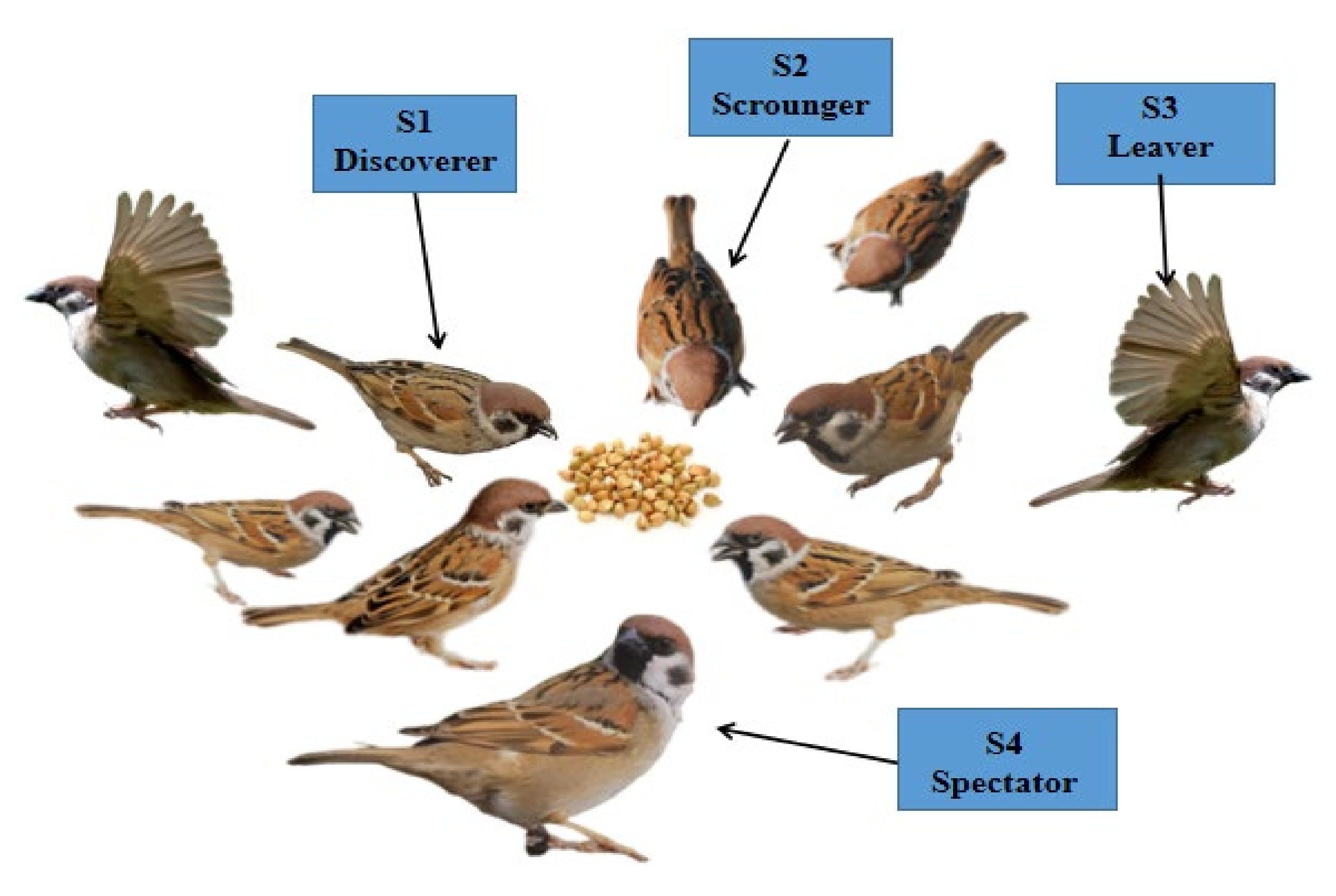
According to the original foraging principle of sparrow populations, a discoverer–scrounger model was established [54]. The interrelationships between individuals in the sparrow population are shown in Figure 5. Generally, the discoverer S1 is responsible for finding food and safe areas, while the scrounger S2 tracks the location of S1 to obtain food, and their roles are constantly changing [55,56]. S3 represents the sparrow at the edge of feeding area. It may leave the location and find another place because it is in the most dangerous position. S4 is responsible for detecting the safety of surrounding environment, and other sparrows also pay attention to S4 while eating.

During the foraging and eating process of sparrow groups, individuals monitor each other while constantly observing changes in the surrounding environment [57,58]. If S4 sends a hazard signal to the population, the entire group will scatter away immediately. In addition, sparrows at the edge of community are more likely to be attacked by natural enemies than those at the center, so they will spontaneously and constantly adjust their positions to ensure safety.

According to the above idea, the SSA model can be established. Assuming that the sparrow population is in the space of $N\times D$, it can be defined by:

$$X=\left[\begin{array}{c}{X}_1\\ X_2\\ ⋮\\ X_n\\ ⋮\\ X_N\end{array}\right]=\left[\begin{array}{cccccc}{x}_{1,1}& x_{1,2}& \dots & x_{1,d}& \cdots & x_{1,D}\\ x_{2,1}& x_{2,2}& \dots & x_{2,d}& \dots & x_{2,D}\\ ⋮& ⋮& ⋮& ⋮& ⋮& ⋮\\ x_{n,1}& x_{n,2}& \dots & x_{n,d}& \dots & x_{n,D}\\ ⋮& ⋮& ⋮& ⋮& \ddots & ⋮\\ x_{N,1}& x_{N,2}& \dots & x_{N,d}& \dots & x_{N,D}\end{array}\right],n=1,2,3,\dots ..,N$$

(1)

where x is the position of sparrows, D indicates the spatial dimension, and N represents the number of total sparrows.

The fitness value indicates the energy reserve, which is defined as:

$$F_X=\left[\begin{array}{c}{f}_1\\ f_2\\ ⋮\\ f_n\\ ⋮\\ f_N\end{array}\right]=\left[\begin{array}{cccccc}f\left[x_{1,1}\right.& x_{1,2}& \cdots & x_{1,d}& \cdots & \left.x_{1,D}\right]\\ f\left[x_{2,1}\right.& x_{2,2}& \cdots & x_{2,\mathrm{d}}& \cdots & \left.x_{2,D}\right]\\ ⋮& ⋮& ⋮& ⋮& ⋮& ⋮\\ f\left[x_{n,1}\right.& x_{n,2}& \cdots & x_{n,\mathrm{d}}& \cdots & \left.x_{n,D}\right]\\ ⋮& ⋮& ⋮& ⋮& \ddots & ⋮\\ f\left[x_{N,1}\right.& x_{N,2}& \cdots & x_{N,d}& \cdots & \left.x_{N,D}\right]\end{array}\right],n=1,2,3,\dots ..,N$$

(2)

Generally, the discoverer S1 has a larger foraging range than the scrounger S2, and updates its position constantly. The update process can be calculated as:

$$X_{nd}^{t+1}=\left\{\begin{array}{cc}{X}_{nd}^t\cdot \exp \left(\frac{-n}{\alpha \cdot P}\right),\hfill & R_2<ST\\ X_{nd}^t+Q\cdot L,\hfill & R_2\ge ST\end{array}\right.$$

(3)

where $t$ denotes the current number of iterations; $P$ refers to the maximum number of iterations; $\alpha$ is a random number of $[0,1]$; $R_2$ is the warning threshold, and $R_2\in [0,1]$; $ST$ indicates the safety value, and $ST\in [0.5,1]$; $Q$ represents a random number that follows the normal distribution; $L$ shows a $1\times d$ matrix in which each element is 1; and $X_{nd}^{}$ signifies the position of a sparrow.

When $R_2<ST$, it indicates the current foraging area is safe, and the sparrows can continue to eat, so the foraging range can be expanded. When $R_2\ge ST$, the spectators find the predator and immediately issue an alarm signal, then all sparrows will scatter away immediately.

The location of scroungers S2 is also updated accordingly because the central location is more secure. The update equation is indicated as:

$$X_{n,d}^{t+1}=\left\{\begin{array}{cc}Q\cdot \exp \left(\frac{X_{worst}^t-X_{n,d}^t}{n^2}\right),\hfill & \hfill n>\frac{N}{2}\\ X_{best}^{t+1}+\left|X_{n,d}^t-X_{best}^{t+1}\right|\cdot A^{+}\cdot L,\hfill & \hfill n\le \frac{N}{2}\end{array}\right.$$

(4)

where $X_{worst}^t$ represents the global worst position; $X_{n,d}^t$ is the best position occupied by the discoverer; and $A$ represents a 1 × d matrix in which the elements are randomly assigned to be 1 or −1, and $A^{+}=A^T{\left(A{A}^T\right)}^{-1}$.

When $n>\frac{N}{2}$, it means that the $n^{th}$ scrounger with a poor fitness value is hungry, and should fly in other directions to find food.

The spectators S4 generally account for 10% to 20% of the population. When danger approaches, they will scatter away and move to a new location. The position-update equation is:

$$X_{n,d}^{t+1}=\left\{\begin{array}{c}{X}_{best}^t+\beta \left(X_{n,d}^t-X_{best}^t\right),\begin{array}{cc}\begin{array}{cc}& \end{array}& f_n\ne f_g\end{array}\\ X_{n,d}^t+K\cdot \left(\frac{X_{n,d}^t-X_{worst}^t}{\left|f_n-f_w\right|+e}\right),\begin{array}{cc}& f_n=f_g\end{array}\end{array}\right.$$

(5)

where $X_{best}^t$ represents the global safest position; $\beta$ and $K\in [-1,1]$ are both control parameters of step length, while $\beta$ is a random number that follows the normal distribution with a mean value of 0 and variance of 1, and $K\in [-1,1]$ represents the direction of sparrow movement; $f_n$, $f_g$, and $f_w$ respectively represent the current fitness value of a sparrow, the global optimal value, and the global worst value; and e is a constant to prevent the denominator from being 0.

When $f_n>f_g$, it means the sparrow is at the edge of the population and is vulnerable to predators. When $f_n=f_g$, it indicates the sparrow in the middle of the population is aware of the danger and needs to be close to other sparrows to reduce the probability of being preyed upon.

3.2. Sparrow Search Algorithm–Back Propagation Neural Network (SSA-BPNN) Model

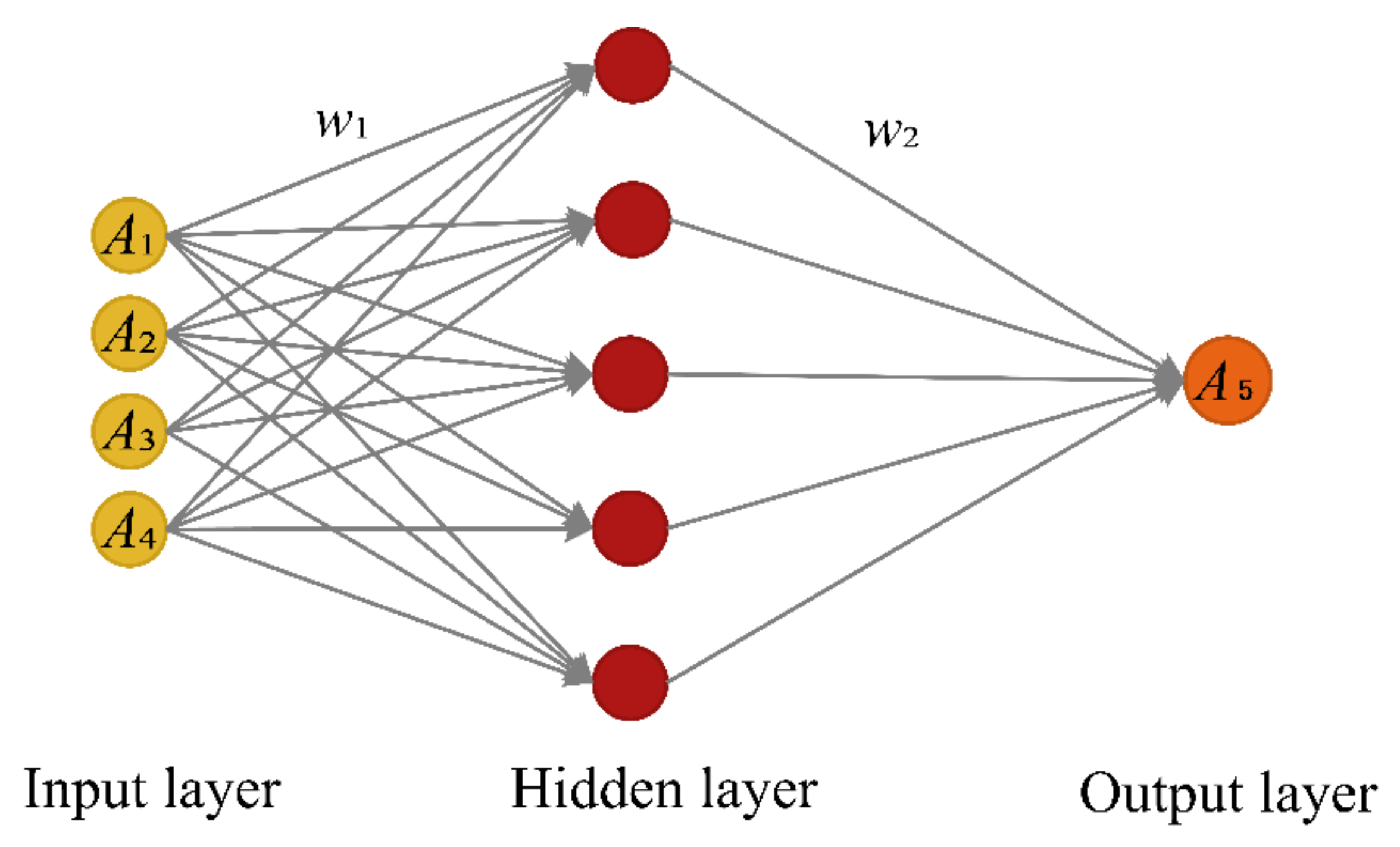
The calculation process of a BPNN is similar to nonlinear mapping, which uses multiple neurons to form a multilayer feedback model. The characteristics of the data are obtained through the continuous iteration of the algorithm. BPNN has a high learning adaptability, and can predict unknown data based on a previously learned pattern [59,60,61,62,63].

However, a BPNN has the defect of being easy to converge to a local minimum when fitting nonlinear functions. The SSA provides a new method to solve the parameter-optimization problem of a BPNN. In the SSA-BPNN model, the SSA reduces the error by continuously adjusting the weight and threshold of each layer, and improves the convergence speed.

The steps for an SSA to optimize a BPNN are as follows:

Step 1: The relevant parameters of the BPNN are initialized;

Step 2: The relevant parameters of the sparrow population are initialized, and the maximum number of iterations $P$ is defined;

Step 3: Based on the fitness values, the sparrows are sorted to generate initial population positions. The mean-square error (MSE) is selected as the fitness function;

Step 4: According to Equations (3)–(5), the positions of discoverer S1, scrounger S2, and spectator S4 are updated;

Step 5: The current updated position is obtained. If the new position is better than the old position from a previous iteration, the update operation is performed; otherwise, the iterative process continues until the condition is met. Finally, the best individual and fitness values are obtained;

Step 6: The global optimal individual is used as the weight of the BPNN, and the global optimal solution is adopted as the threshold of the BPNN;

Step 7: When the number of iterations is reached or the error is met, the calculation process stops; otherwise, the program re-executes beginning at step 3.

3.3. Sparrow Search Algorithm–Elman Neural Network (SSA-ENN) Model

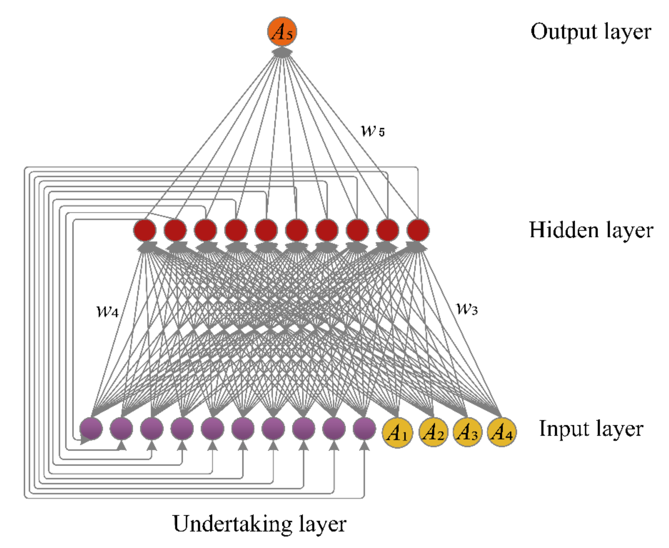
An ENN is a dynamic recurrent neural network that adds local memory units on the basis of a traditional feedforward network [64,65]. In addition to the hidden layer, it inserts an undertaking layer to the original grid that is used as a one-step delay operator to record dynamic information. Therefore, it obtains the ability to adapt to time-varying characteristics. Compared with traditional neural networks, it has better learning capabilities and can be used to solve problems including optimization, fitting, and regression.

However, an ENN has the randomness problem with initial weights and thresholds, which affects the accuracy of its predictions. In this study, an SSA was used to optimize the initial weights and thresholds of an ENN to improve the overall predictive performance.

The stages of SSA optimization of an ENN are as follows:

Stage 1: Initialize the relevant parameters of ENN and SSA;

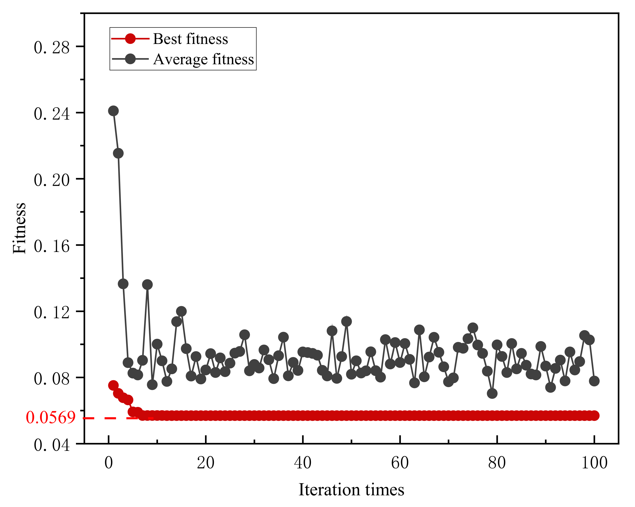
Stage 2: Calculate the fitness of initial population and sort the results. The best and worst individuals can be determined. MSE is selected as the fitness function;

Stage 3: According to Equations (3)–(5), the positions of sparrows S1, S2, and S4 are updated based on fitness ranking;

Stage 4: Calculate the fitness value. The position of each sparrow is updated constantly. If the stop condition is met, the iterative process stops. Otherwise, the above process should be repeated;

Stage 5: Obtain the optimal weights and thresholds of the ENN.

3.4. Sparrow Search Algorithm–Support Vector Regression (SSA-SVR) Model

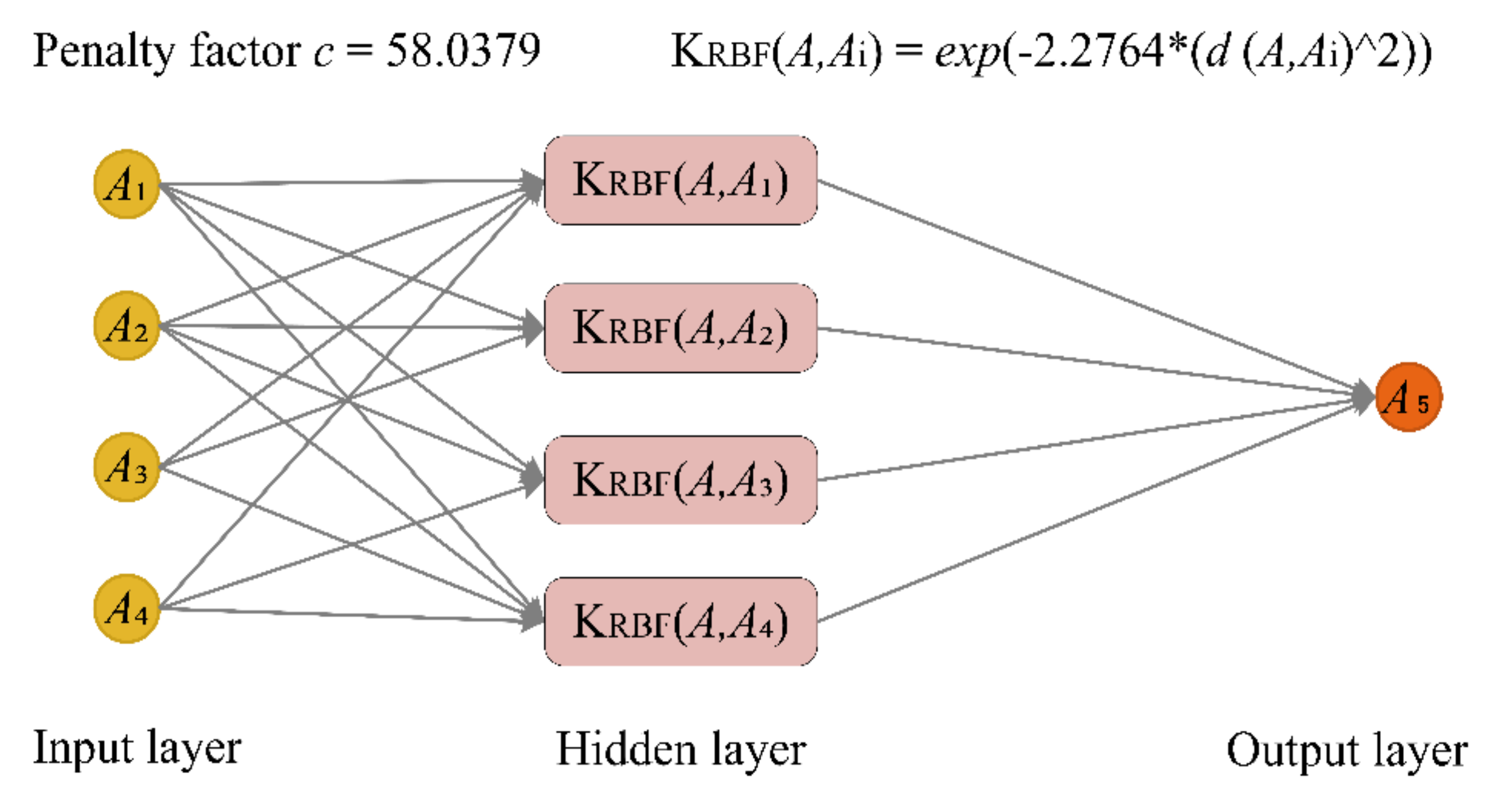
An SVR model mainly includes two steps. First, the nonlinear data is mapped into a high-dimensional space through the kernel function to make the data linearly separable. Then, the data is processed based on the principle of structural risk minimization.

Two important parameters in the SVR model include the penalty parameter $c$ and the kernel function parameter $g$. Among them, $c$ represents the error tolerance and $g$ indicates the learning ability. The higher the value of $c$, the smaller the tolerance to error, and the more likely to overfit. In addition, $g$ affects the prediction accuracy directly. Therefore, it is necessary to determine the optimal $c$ and $g$ during the training process.

The stages of SSA optimization of an SVR are as follows:

Stage 1: Build and initialize the SVR model;

Stage 2: Initialize the parameters of SSA, and determine the range of $c$ and $g$;

Stage 3: Calculate the fitness of the initial population and determine the best and worst individuals. MSE is selected as the fitness function;

Stage 4: Update the positions of sparrows S1, S2, and S4 based on Equations (3)–(5);

Stage 5: Calculate the fitness value and update the position of the sparrows. The iterative process will break when the stop condition is met. Otherwise, the above steps will be repeated;

Stage 6: Obtain the optimal $c$ and $g$, which are then used for model training.

3.5. Model Evaluation Indexes

In order to evaluate model performance, seven indexes, including MAE, R², NSC, MAPE, Theil’s U value, RMSE, and SSE, were adopted.

MAE represents the average error between predicted value and actual value. The calculation equation is [66]:

$$\mathrm{MAE}=\frac{1}{n}{\displaystyle \sum _{i=1}^n\left|f_i-y_i\right|}$$

(6)

where $n$ is the number of samples; $f_i$ and $y_i$ are the predicted value and actual value of the $i^{th}$ sample, respectively; and $\overline{y}$ denotes the average of the actual values.

R² is used to indicate the correlation between two variables. The calculation equation is [33]:

$${\mathrm{R}}^2=\frac{(n{\displaystyle \sum _{i=1}^n{f}_i{y}_i}-{\displaystyle \sum _{i=1}^n{f}_i{\displaystyle \sum _{i=1}^n{y}_i}}{)}^2}{(n{\displaystyle \sum _{i=1}^n{\left(f_i\right)}^2}-({\displaystyle \sum _{i=1}^n{f}_i{)}^2})(n{\displaystyle \sum _{i=1}^n{\left(y_i\right)}^2-}({\displaystyle \sum _{i=1}^n{y}_i{)}^2})}$$

(7)

NSC is used to describe the predictive efficiency. The calculation equation is [67]:

$$\mathrm{NSC}=1-\frac{{\displaystyle \sum _{i=1}^n{\left(y_i-f_i\right)}^2}}{{\displaystyle \sum _{i=1}^n{\left(y_i-\overline{y}\right)}^2}}$$

(8)

Theil’s U value is used to indicate the prediction accuracy. The calculation equation is [68]:

$$\mathrm{Theil}’\mathrm{s} \mathrm{U}=\frac{\sqrt{\frac{1}{n}{\displaystyle {\sum }_{i=1}^n{\left(y_i-f_i\right)}^2}}}{\sqrt{\frac{1}{n}{\displaystyle {\sum }_{i=1}^n{y}_i{}^2}}+\sqrt{\frac{1}{n}{\displaystyle {\sum }_{i=1}^n{f}_i{}^2}}}$$

(9)

MAPE denotes the average value of the relative error. The calculation equation is [69]:

$$\mathrm{MAPE}=\frac{1}{n}{\displaystyle \sum _{i=1}^n\left|\frac{f_i-y_i}{y_i}\right|}\times 100\%$$

(10)

RMSE is used to describe the deviation between the predicted value and actual value. The calculation equation is [70]:

$$\mathrm{RMSE}=\sqrt{\frac{1}{n}{\displaystyle \sum _{i=1}^n{\left(f_i-y_i\right)}^2}}$$

(11)

SSE is used to calculate the sum of the squared error. The calculation equation is [71]:

$$\mathrm{SSE}={\displaystyle \sum _{i=1}^n{\left(y_i-f_i\right)}^2}$$

(12)

4. Results and Analysis

4.1. Results of SSA-BPNN Model

A three-layer grid was used to establish the SSA-BPNN model. Based on the input and output of the model, the number of nodes in the input and output layers were determined as 5 and 1. In addition, the number of nodes in the hidden layer was obtained based on the MSE of the training set. By setting the number of nodes from 3 to 15, the MSE of the training set was obtained, as shown in Figure 6. It can be seen that the MSE was the smallest when the number of nodes was 5. Therefore, the grid structure of the SSA-BPNN model was chosen as $4-5-1$, as shown in Figure 7.

In order to obtain a better predictive performance, other grid parameters, such as the number of trainings, minimum error of training target, initial population size of the SSA, and maximum evolutionary generation, were optimized by trial and error and set to 1000, 0.0001, 30, and 100, respectively. Then, the SSA was used to optimize the weights and thresholds of the BPNN model, and the optimized weight matrices $w_1$ and $w_2$ were obtained as follows:

$$w_1=\left[\begin{array}{cccc}0.1089& -0.2795& 0.2414& -0.7100\\ 0.0890& -11.3880& 7.6001& 1.5449\\ 0.3197& 0.4036& -0.0070& -0.4563\\ -6.0878& 0.7283& 0.1796& 1.3281\\ -0.6581& -2.0707& 11.9725& 10.5624\end{array}\right]$$

(13)

$$w_2=\left[\begin{array}{ccccc}-2.6242& -0.2653& -4.0481& -0.2858& -0.4481\end{array}\right]$$

(14)

After the model was trained based on the training set, the test set was used to evaluate the predictive performance of the SSA-BPNN model. The relationship between the actual and predicted values is shown in Figure 8. It can be seen that their values had a good correlation.

In addition, the predictive performance of the BPNN model before and after the SSA optimization was compared. Seven performance evaluation indexes, including MAE, R², NSC, MAPE, Theil’s U value, RMSE, and SSE, were calculated, as shown in

Table 3. Evaluation index values of BPNN and SSA-BPNN models.

Model	MAE	R2	NSC	MAPE	Theil’s U Value	RMSE	SSE
BPNN	0.2169	0.7425	−3.8026	15.4075%	0.0144	0.2873	3.4665
SSA-BPNN	0.1246	0.9277	−1.2331	8.4127%	0.0084	0.1636	1.1241

. According to these index values, the SSA-BPNN model performed better than the BPNN model. The absolute error of the different samples was determined, as demonstrated in Figure 9. Overall, the absolute error of the SSA-BPNN model was smaller and more stable than that of the BPNN model. At the same time, the maximum error of the BPNN model was larger. Therefore, SSA improved the predictive performance of the BPNN model to some extent.

4.2. Results of SSA-ENN Model

To establish the optimal grid structure, SSA-ENN models with different numbers of hidden layer nodes were built. The training error was determined when the number of nodes was selected from 3 to 12, as shown in Figure 10. When the number of hidden layer nodes was 10, the error was the smallest. Therefore, the grid structure of the SSA-ENN model was selected as $4-10-10-1$, as shown in Figure 11.

For training the model, other grid parameters, such as the learning rate, minimum error of training target, and initial population size of SSA, were optimized by trial and error and set to 0.01, 0.0001, and 30, respectively. Then, the weights and thresholds of the ENN were optimized by the SSA based on the training set, and the optimized weight matrices $w_3$, $w_4$, and $w_5$ were obtained as follows:

$$w_3=\left[\begin{array}{cccc}-2.0388& -1.5616& -0.1513& 1.3243\\ 1.0527& -0.0656& -0.7647& -2.0608\\ -2.6026& -0.0921& -1.1416& -3.2409\\ 0.2770& 0.4636& -1.1443& -1.8673\\ -0.4656& -1.4285& -0.0750& -0.7841\\ -1.9833& 0.1517& -0.6582& -0.5568\\ -0.5375& -1.6703& 0.1149& 0.6181\\ -0.3918& 0.7763& -2.5244& -1.8498\\ 0.0175& -2.2129& -1.1439& -1.3245\\ -2.1403& -0.4759& -0.2951& -2.0509\end{array}\right]$$

(15)

$$w_4=\left[\begin{array}{cccccccccc}\hfill -0.6309& -0.5862& -0.636& -0.6344& -0.71& -0.6323& -0.665& -0.7285& -0.6339& -0.6346\\ \hfill -0.6356& -0.6129& -0.632& -0.7323& -0.6546& -0.6458& -0.627& -0.7207& -0.759& -0.6144\\ \hfill -0.582& -0.7272& -0.683& -0.7091& -0.6001& -0.6132& -0.654& -0.6353& -0.6318& -0.5988\\ \hfill -0.708& -0.613& -0.635& -0.6603& -0.6202& -0.6294& -0.636& -0.6121& -0.6181& -0.597\\ \hfill -0.5904& -0.633& -0.644& -0.668& -0.6803& -0.6779& -0.635& -0.6116& -0.6568& -0.6448\\ \hfill -0.6247& -0.6524& -0.631& -0.6138& -0.6359& -0.7771& -0.667& -0.6259& -0.634& -0.6419\\ \hfill -0.6149& -0.6013& -0.691& -0.6621& -0.6069& -0.7022& -0.678& -0.633& -0.5831& -0.691\\ \hfill -0.6466& -0.6066& -0.643& -0.6517& -0.7294& -0.7349& -0.668& -0.6627& -0.6243& -0.6588\\ \hfill -0.6707& -0.5838& -0.645& -0.6155& -0.6464& -0.6233& -0.64& -0.5822& -0.6532& -0.6794\\ \hfill -0.6237& -0.631& -0.602& -0.644& -0.658& -0.6256& -0.63& -0.638& -0.6506& -0.702\end{array}\right]$$

(16)

$$w_5=\left[0.9634\hspace{1em}1.5589\hspace{1em}1.4220\hspace{1em}-1.5235\hspace{1em}-1.1393\hspace{1em}0.7611\hspace{1em}-1.3683\hspace{1em}0.3639\hspace{1em}1.3427\hspace{1em}-1.8511\right]$$

(17)

The test set was used to evaluate the predictive performance of the SSA-ENN model. The relationship between the actual and predicted values is shown in Figure 12. It can be observed that the predicted value was very close to the actual value.

In order to compare the predictive performance of the ENN and SSA-ENN models, their performance evaluation indexes were calculated, as shown in

Table 4. Evaluation index values of ENN and SSA-ENN models.

Model	MAE	R2	NSC	MAPE	Theil’s U Value	RMSE	SSE
ENN	0.2210	0.6824	−5.4164	15.5604%	0.0175	0.3429	4.9377
SSA-ENN	0.1215	0.9204	−1.3872	8.6297%	0.0088	0.1735	1.2646

. All index values indicated that the SSA-ENN performed better than the ENN. In particular, the R² increased from 0.6824 to 0.9204, and the MAPE decreased from 15.5604% to 8.6297%. The absolute error of each sample in the test set was obtained, as shown in Figure 13. It can be seen that the error of the SSA-ENN was around zero, but the error of the ENN was larger and relatively unstable. Therefore, the ENN model optimized by the SSA had a better accuracy.

4.3. Results of SSA-SVR Model

The SSA was used to optimize the parameters $c$ and $g$ of the SVR model. The population size of the SSA, the maximum number of iterations, and the cross-validation fold were set to 20, 100, and 5, respectively. Then, the best values of $c$ and $g$ were determined as 58.0379 and 2.2764, and the corresponding MAE of the cross-validation was 0.0569. The structure of the SSA-SVR model is shown in Figure 14 Then, the test set was adopted to assess the predictive performance of the SSA-SVR model. The fitting relation of the actual and predicted values is shown in Figure 15.

The variation of fitness (MSE) with the number of iterations is shown in Figure 16. It can be seen that as the number of iterations increased, the fitness decreased. Especially in the first five generations, the fitness decreased rapidly. At the 12th iteration, the optimal fitness value was obtained as 0.0569.

The traditional SVR model was also used for a comparison. Based on the cross-validation results, the values of $c$ and $g$ were determined to be 1024 and 0.0078, respectively, and the MAE was 0.2647. Seven performance evaluation indexes for the SVR and SSA-SVR models were calculated, as shown in

Table 5. Evaluation index values of SVR and SSA-SVR models.

Model	MAE	R2	NSC	MAPE	Theil’s U Value	RMSE	SSE
SVR	0.3978	0.3699	−2.7614	28.3285%	0.0225	0.4568	8.7640
SSA-SVR	0.1856	0.8261	−4.6656	12.8829%	0.0122	0.2386	2.3907

. Based on these index values, the SSA-SVR model had a better predictive performance. The absolute error corresponding to each sample is displayed in Figure 17. It can be seen that the prediction results of the SSA-SVR model were closer to the actual value. Therefore, the predictive performance of the SVR model was improved by the SSA.

5. Discussion

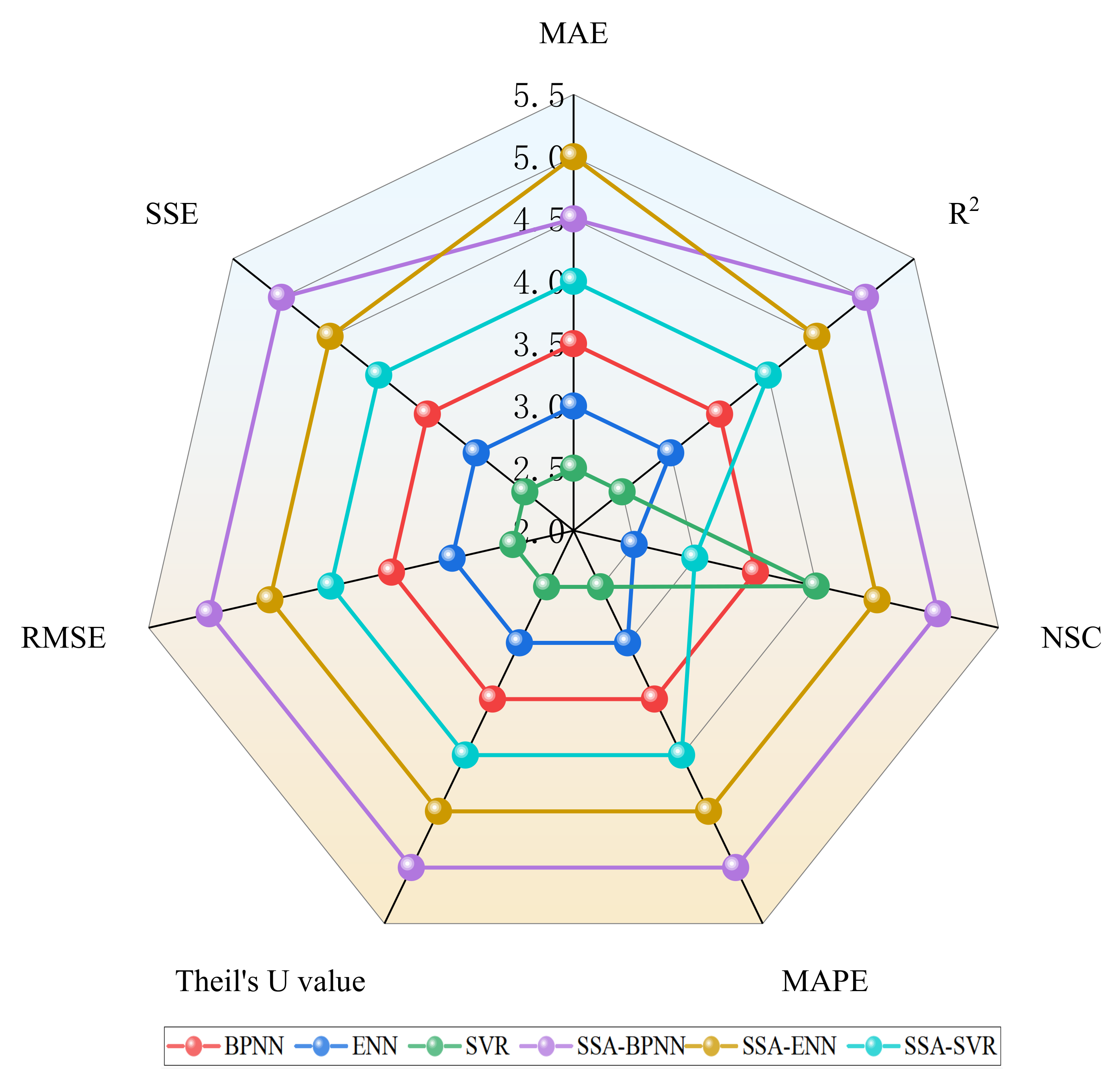
The main purpose of this study was to select an appropriate model to predict the thickness of an EDZ. Although these models were comprehensively evaluated based on seven evaluation indexes, as shown in Table 3, Table 4 and Table 5, it was necessary to determine their ranking results. In order to obtain the predictive performance of each model more intuitively, a score method was proposed. The specific scoring principle was that the best model in each index was given 5 points, the second-ranked model was given 4.5 points, and the lower-ranked models’ scores were sequentially reduced by 0.5 points. 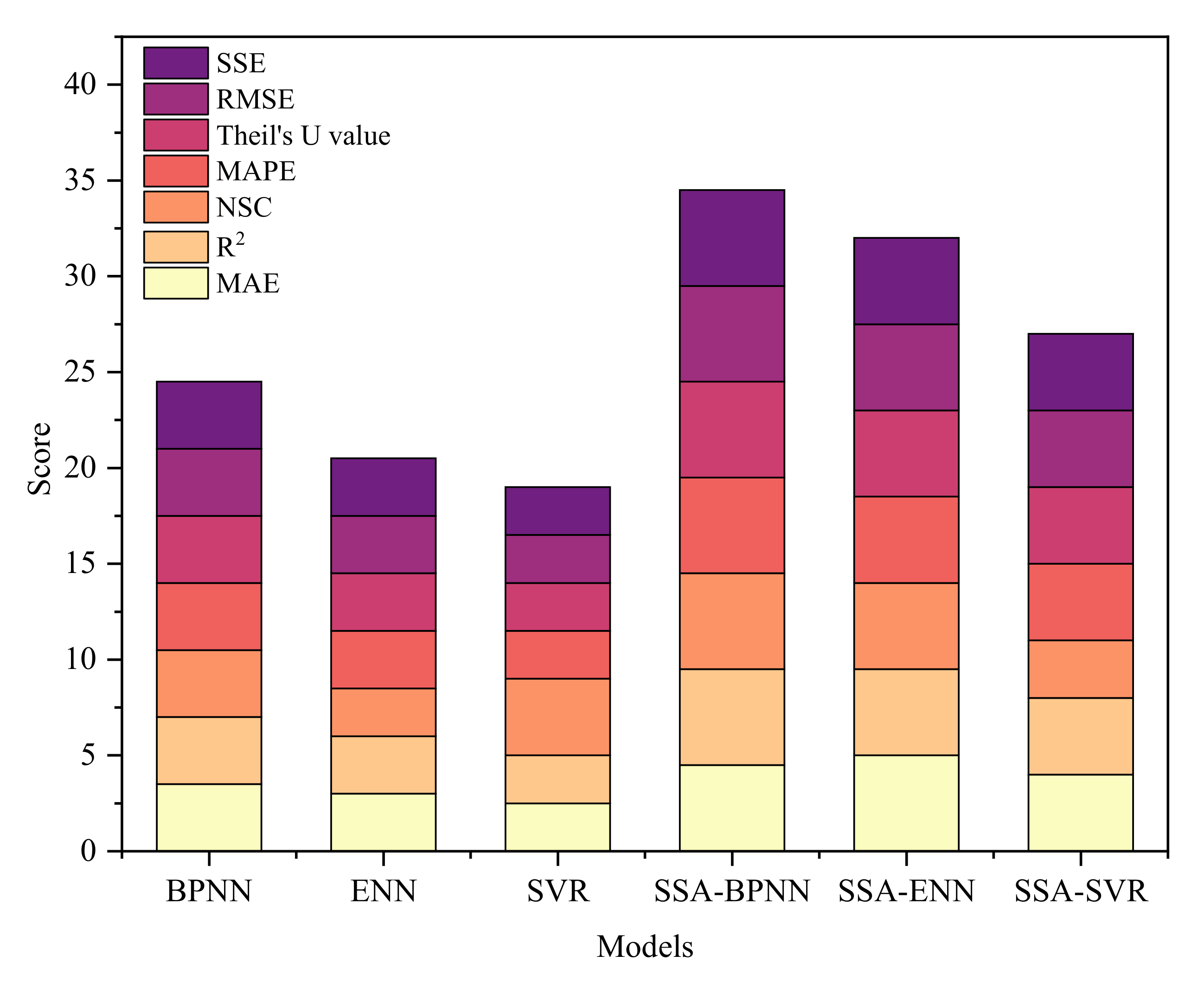The radar chart of the model score corresponding to each index is shown in Figure 18. It can be seen that most of the scores for each model index were basically at the same level. According to the area of the radar chart, it can clearly be seen that the SSA-BPNN and SSA-ENN models performed better. Based on the scores of various indexes, a stacked chart was obtained, as shown in Figure 19. It can be seen that the scores of the models optimized by SSA increased significantly, which illustrated the importance of parameter optimization with the SSA. According to the total scores, the ranking results were determined as SSA-BPNN > SSA-ENN > SSA-SVR > BPNN > ENN >SVR. The SSA-BPNN model was more suitable for predicting the thickness of an EDZ.

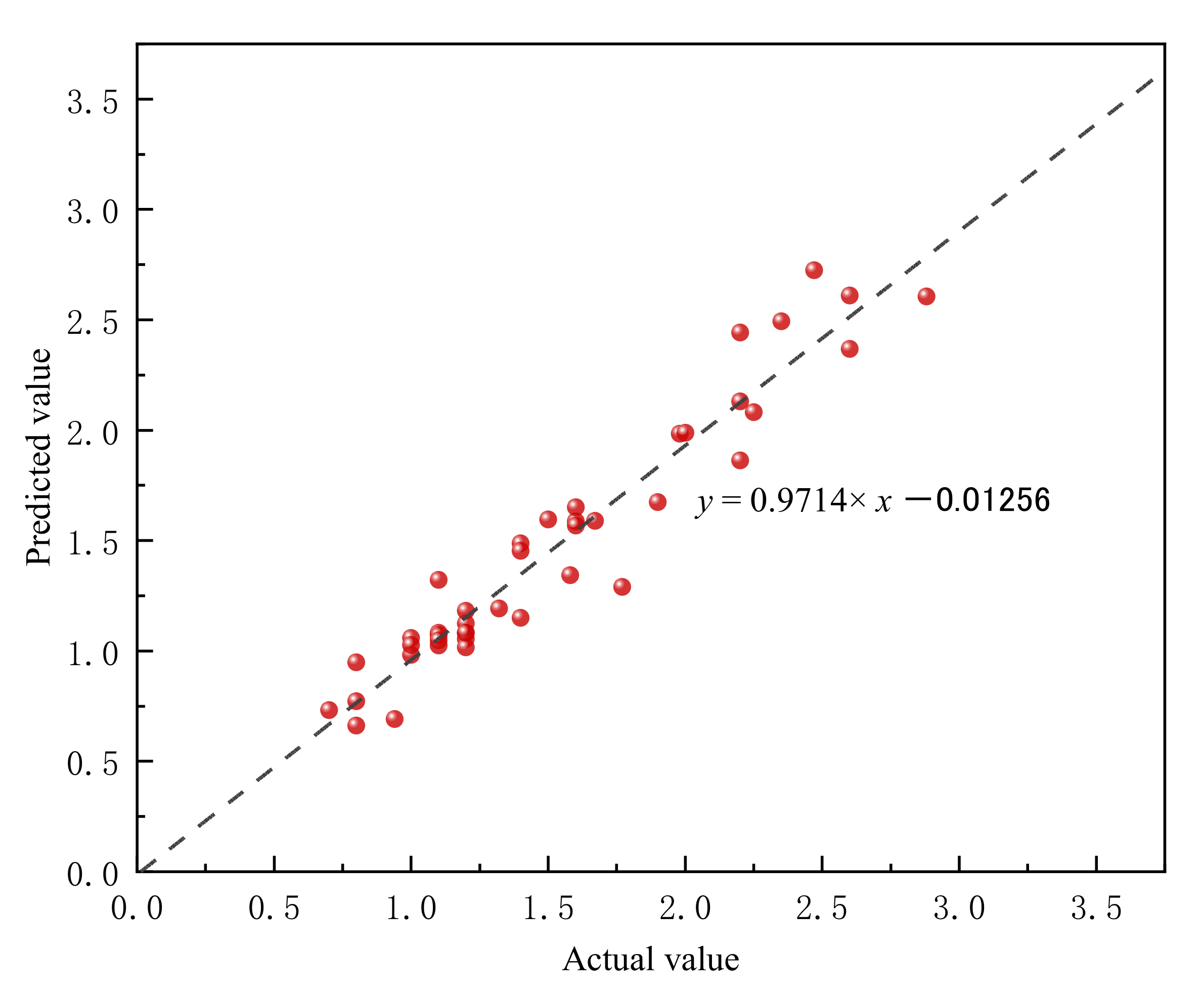
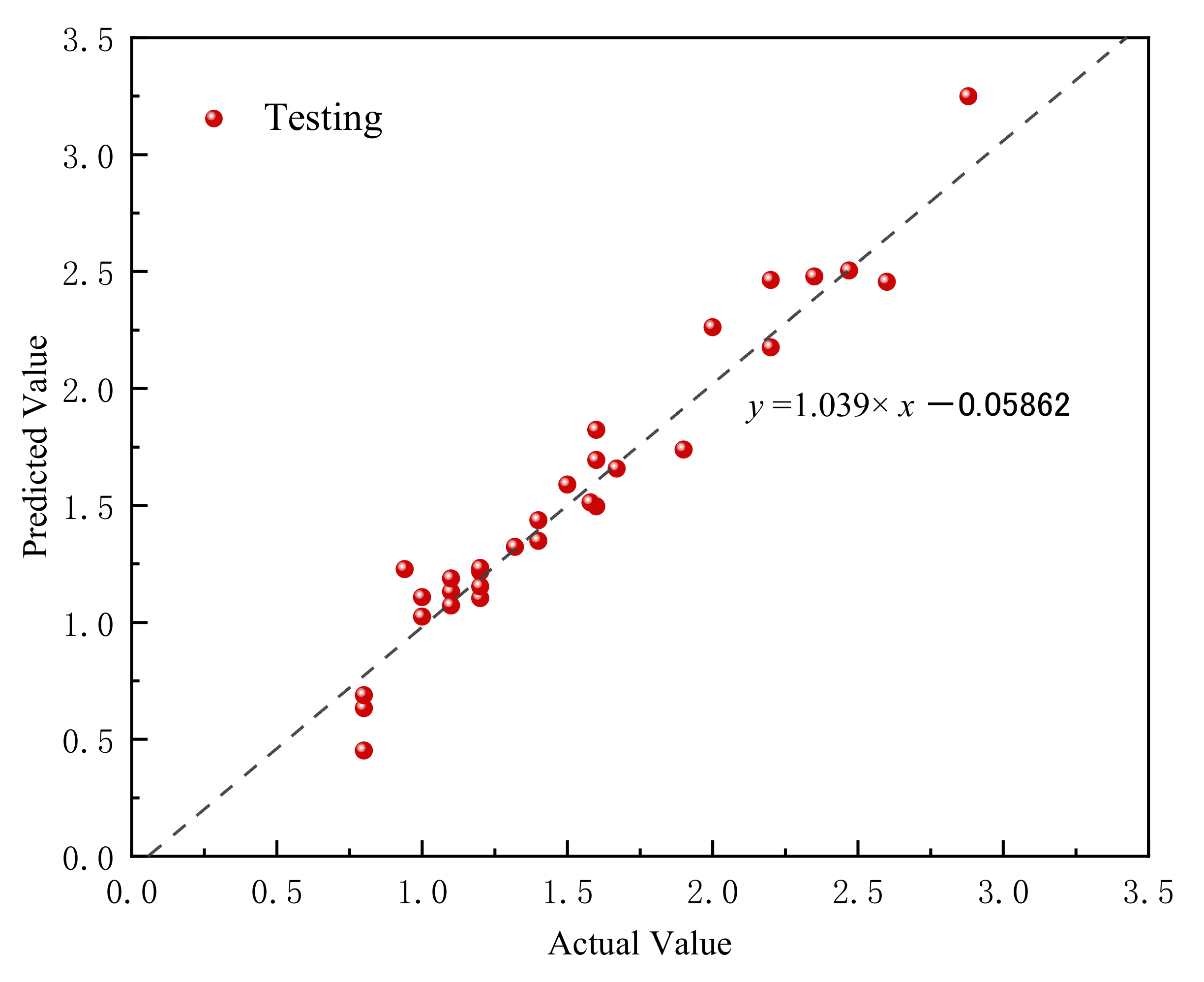
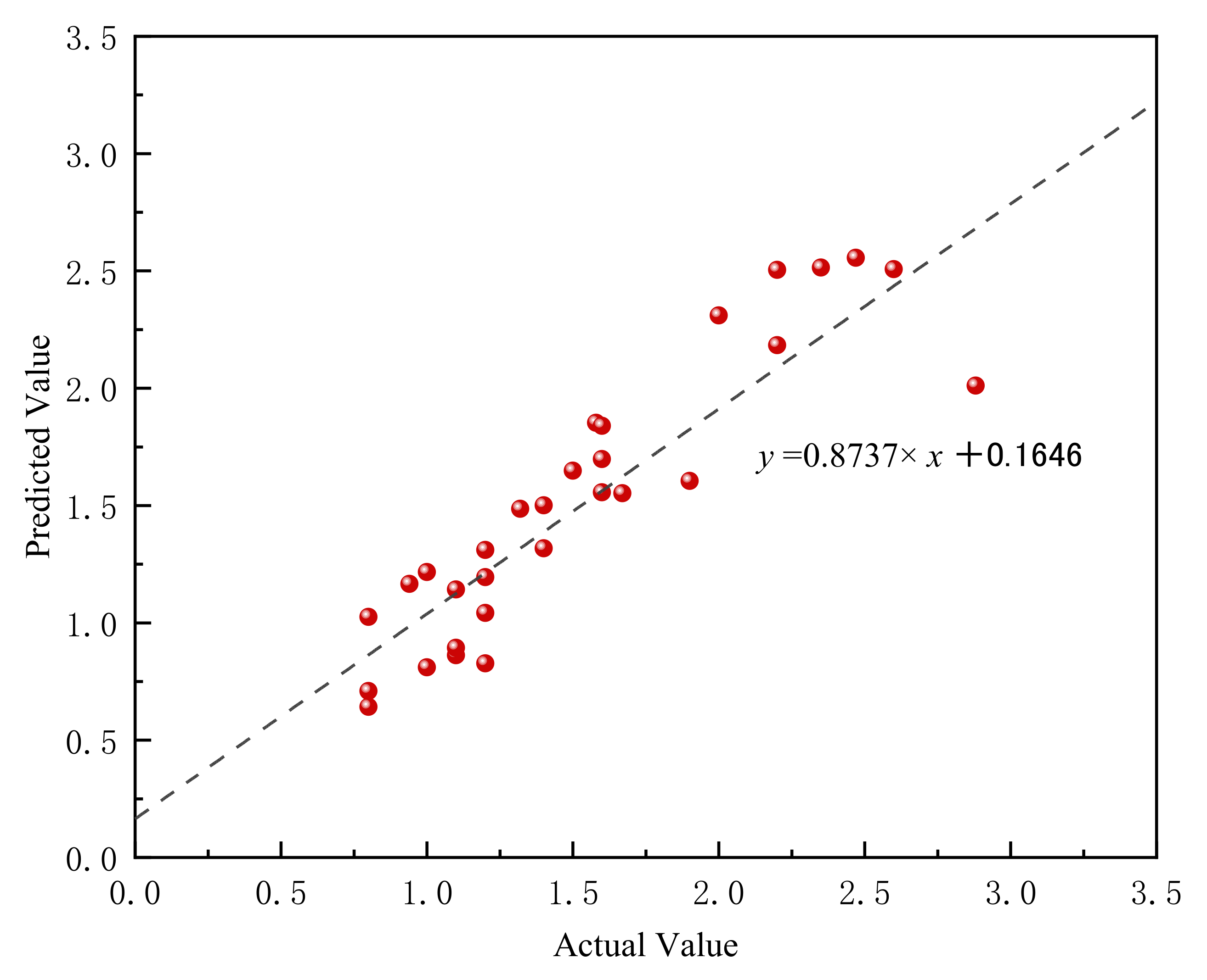
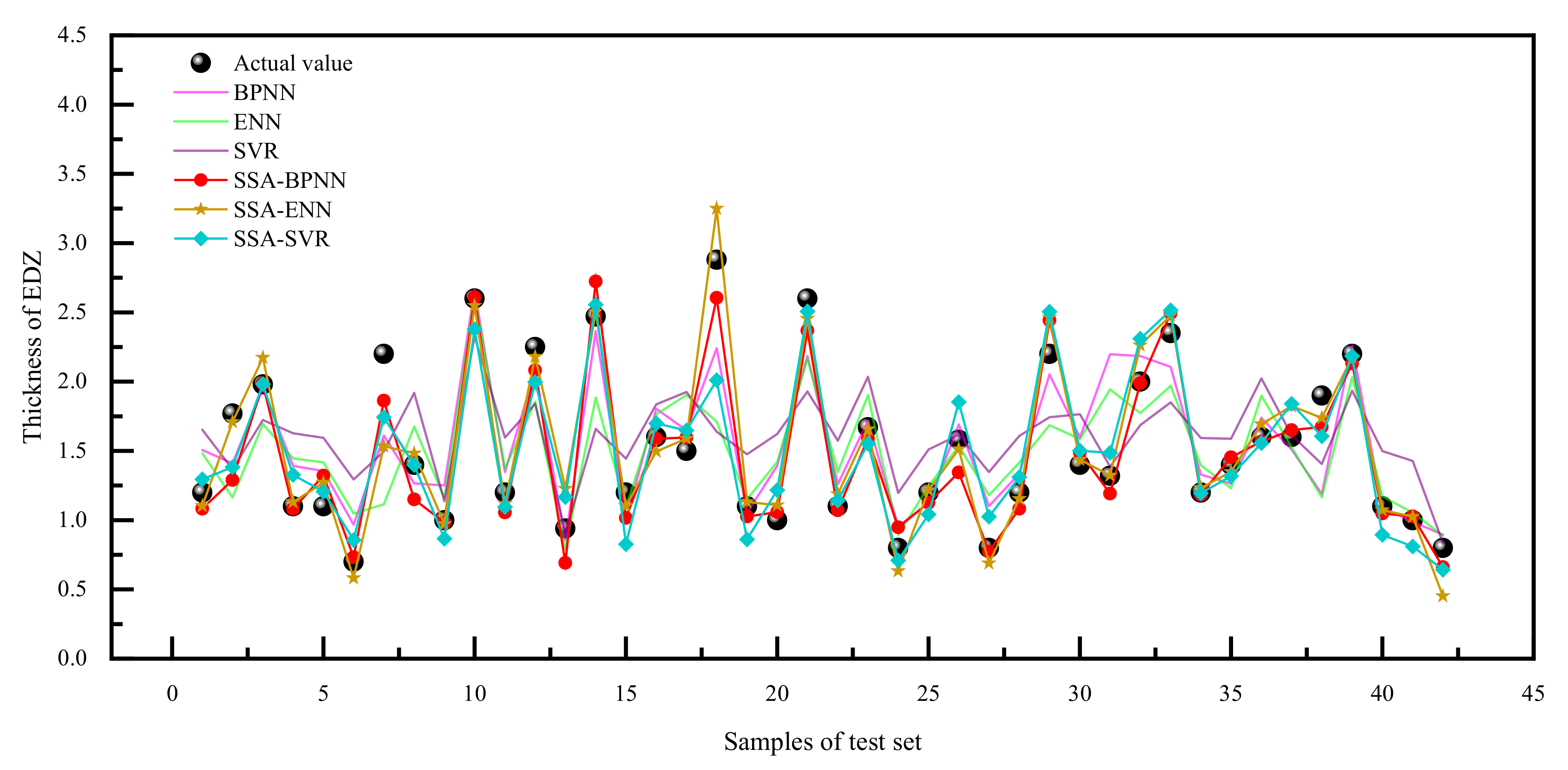
In addition, the predicted and actual values of each model were compared, as shown in Figure 20. In the figure, it can be seen that the predicted results of the SSA-BPNN model were closer to the actual value. Combined with the scoring principle, we determined that the SSA-BPNN model had the highest accuracy.

In order to further verify the reliability of the proposed model, it was necessary to compare it with the empirical-formula method. Zhao et al. [21] proposed an empirical formula to determine the thickness of an EDZ as follows:

$$A_5=0.0145A_1{A}_4{}^{0.9324}{(\frac{\gamma A_1}{A_3})}^{0.4459}{(\frac{{\sigma }_{{}_{H\max }}}{A_3})}^{-0.4308}{(\frac{A_2}{A_1})}^{0.5334}$$

(18)

where $\gamma$ is the unit weight of rock and ${\sigma }_{{}_{H\max }}$ is the maximum horizontal principal stress.

This empirical formula adopts six indicators, such as $A_1$, $A_2$, $A_3$, $A_4$, $\gamma$, and ${\sigma }_{{}_{H\max }}$. Because some of its indicators are the same as those in this study, this empirical formula could be adopted to compare with the proposed model. The data in reference [21] were used to evaluate the predictive performance, and the predicted results are shown in

Table 6. Predictive performance of SSA-BPNN model and empirical formula.

Mine	${\mathit{A}}_{\mathbf{1}}$/m	${\mathit{A}}_{\mathbf{2}}$/m	${\mathit{A}}_{\mathbf{3}}$/MPa	${\mathit{A}}_{\mathbf{4}}$	$\mathit{\gamma }$/(KN/m3)	${\mathit{\sigma }}_{{}_{\mathit{H}\mathbf{max}}}$/MPa	${\mathit{A}}_{\mathbf{5}}$/m	MAPE of Empirical Formula	MAPE of SSA-BPNN Model
Maluping Phosphate Mine	660	4.5	34.37	4	27.2	34.49	1.65	9.34%	9.10%
Maluping Phosphate Mine	660	4.0	147.89	5	32.2	34.49	2.34	5.13%	6.27%
Sanshandao Gold Mine	600	3.8	71.26	3	27.1	32.45	1.10	7.27%	2.35%
Jinchuan Nickel Mine	1000	4.60	39.19	3	28.6	50.80	1.93	7.77%	4.68%

. It can be seen that the overall prediction performance of the SSA-BPNN model was better than that of the empirical formula.

Although the proposed models could obtain satisfactory results, there were still some limitations:

(1)

The dataset of EDZ cases was relatively small. The accuracy of a regression model heavily relies on the quantity and quality of the dataset. If the dataset is small, the model may overfit, which will affect its generalization and reliability. Although this study integrated most of the cases in the existing literature, the dataset was still relatively small. Therefore, establishing a more comprehensive EDZ database would be helpful to predict the thickness of an EDZ more efficiently using the proposed models.

(2)

Only four indicators were selected for the thickness prediction of an EDZ. Due to the complexity of EDZ formation, the thickness of an EDZ is affected by various factors. Other indicators, such as the roadway shape, the presence of underground water, and the excavation method, may also have influences on the prediction results. Therefore, it is necessary to investigate the influences of more indicators in the future.

6. Conclusions

Determining the thickness of an EDZ is a crucial issue in the design of roadway support. This study proposed SSA-BPNN, SSA-ENN, and SSA-SVR models for the thickness prediction of EDZ. A dataset including 209 cases from 34 mines was collected to establish the predictive models. An SSA was used to optimize the parameters of the BPNN, ENN, and SVR models. MAE, R², NSC, MAPE, Theil’s U value, RMSE, and SSE were used to evaluate model performance. According to these index values, the ranking result of each model was determined to be: SSA-BPNN > SSA-ENN > SSA-SVR > BPNN > ENN > SVR. Overall, the SSA improved the predictive performance of the traditional BPNN, ENN, and SVR models. The proposed models obtained satisfactory results and were more suitable for the thickness prediction of an EDZ. The SSA-BPNN model had the best comprehensive performance. The MAE, R², NSC, MAPE, Theil’s U value, RMSE, and SSE were 0.1246, 0.9277, −1.2331, 8.4127%, 0.0084, 0.1636, and 1.1241, respectively. The prediction results provided an important reference for the determination of EDZ thickness.

In the future, a more comprehensive and higher-quality EDZ database should be developed. In addition, it is necessary to analyze the influences of other indicators, especially the excavation method, on the prediction results. Considering the complexity of an EDZ, other swarm-intelligence or ML algorithms can be used for comparison.

References

1. Jing, H.; Meng, Q.; Zhu, J.; Meng, B.; Wei, L. Advances in theories and technologies for stability control of the loose zone of surrounding rock in deep roadways. J. Min. Safety Eng. 2020, 37, 429–442. [Google Scholar]
2. Dong, F.; Guo, Z.; Lan, B. The theory of supporting broken zone in surrounding rock. J. Univ. Sci. Technol. 1991, 2, 64–71. [Google Scholar]
3. Chen, J.; Hu, H.; Zhang, Y. Dynamic and static analysis of mechanism of loosen zone in surrounding rock of tunnels. J. Geotech. Eng. 2011, 33, 1964–1968. [Google Scholar]
4. Dong, F.; Song, H.; Guo, Z. Tunnel wall rock loose circle support theories. J. China Coal Soc. 1994, 19, 21–23. [Google Scholar]
5. Zhao, G.; Wu, H. Support vector machine model of loose ring thickness prediction. J. Guangxi Univ. 2013, 38, 444–450. [Google Scholar]
6. Wang, S.F.; Sun, L.C.; Huang, L.Q.; Li, X.B.; Shi, Y.; Yao, J.R.; Du, S.L. Non-explosive mining and waste utilization for achieving green mining in underground hard rock mine in china. Trans. Nonferrous Met. Soc. China 2019, 29, 1914–1928. [Google Scholar] [CrossRef]
7. Jing, H.; Li, Y.; Liang, J. The mechanism and practice of borehole camera test surrounding rock loose zone. J. Univ. Sci. Technol. 2009, 38, 645–649. [Google Scholar]
8. Song, H.; Wang, C.; Jia, Y. The principle and practice of using ground penetrating radar to test the loose zone of surrounding rock. J. Univ. Sci. Technol. 2002, 4, 43–46. [Google Scholar]
9. Shen, F.; Zhong, W.; Liu, G.; Guo, W. Test and analysis on loose circle of surrounding rock to large distortion region of tong sheng tunnel. J. Eng. Geophys. 2011, 8, 366–369. [Google Scholar]
10. Shin, S.W.; Martin, C.D.; Park, E.S.; Christianson, R. Methodology for estimation of excavation damaged zone around tunnels in hard rock. In Proceedings of the 1st Canada/United States Rock Mechanics Symposium, Vancouver, BC, Canada, 27–31 May 2007. [Google Scholar]
11. Kruschwitz, S.; Yaramanci, U. Detection and characterization of the disturbed rock zone in claystone with the complex resistivity method. J. Appl. Geophys. 2004, 57, 63–79. [Google Scholar] [CrossRef]
12. Zou, H.; Xiao, M. Research on evaluation method of underground cavern excavation loose zone. J. Rock Mech. Geotech. 2010, 29, 513–519. [Google Scholar]
13. Ma, J.; Zhao, G.; Dong, L.; Chen, G.; Zhang, C. A comparison of mine seismic discriminators based on features of source parameters to waveform characteristics. Shock Vib. 2015, 2015, 919143. [Google Scholar] [CrossRef] [Green Version]
14. Liu, G.; Song, H. Numerical simulation of influencing factors of surrounding rock loose zone. Min. Metall. Eng. 2003, 23, 1–3. [Google Scholar]
15. Sun, X.; Chang, Q.; Shi, X.; Li, X. Thickness measurement and distribution law of surrounding rock loose zone in large section semicircular arch coal road. Coal Sci. Technol. 2016, 44, 1–6. [Google Scholar]
16. Perras, M.A.; Diederichs, M.S. Predicting excavation damage zone depths in brittle rocks. J. Rock Mech. Geotech. 2016, 8, 60–74. [Google Scholar] [CrossRef] [Green Version]
17. Wan, C.; Li, X.; Ma, C. Optimization of support technology for deep soft rock roadway based on field measurement of excavation damage zone. Min. Metall. Eng. 2012, 32, 12–16. [Google Scholar]
18. Yan, I. Derivation of excavation damaged zone’s thickness and plastic zone’s scope of tunnel. Jpn. Railw. Tech. Res. Rep. 1974, 900, 1–38. [Google Scholar]
19. Wang, R.; Liang, Y.; Qin, W. Measurement and research on broken zone of surrounding rock in Cha Zhen tunnel. In Proceedings of the 4th International Conference on Civil Engineering, Architecture and Building Materials (CEABM), Haikou, China, 24–25 May 2014; pp. 1321–1326. [Google Scholar]
20. Chen, Q.; Huang, X.; Xie, X. Derivation and improvement of the radius of the loose circle of surrounding rock based on Hoek-Brown criterion. J. Appl. Mech. 2015, 32, 304–310. [Google Scholar]
21. Zhao, G.Y.; Liang, W.Z.; Wang, S.F.; Hong, C.S. Prediction model for extent of excavation damaged zone around roadway based on dimensional analysis. Rock Soil Mech. 2016, 37, 273–278. [Google Scholar]
22. Shemyakin, I.; Fisenko, G.L.; Kurlenya, M.V. Zonal disintegration of rocks around underground workings. III. Theoretical notions. Sov. Min. Sci. 1987, 23, 1–6. [Google Scholar] [CrossRef]
23. Myasnikov, V.P.; Guzev, M.A. Thermomechanical model of elastic-plastic materials with defect structures. Theor. Appl. Fract. Mec. 2000, 33, 165–171. [Google Scholar] [CrossRef]
24. Zhou, X.P.; Song, H.F.; Qian, Q.H. Zonal disintegration of deep crack-weakened rock masses: A non-Euclidean model. Theor. Appl. Fract. Mec. 2011, 55, 227–236. [Google Scholar] [CrossRef]
25. Bao, Y.; Jiang, B.; Ni, T. Theory and numerical simulation of deep rock mass based on a non-euclidean model. Sci. Program.-Neth. 2022, 2022, 4492406. [Google Scholar] [CrossRef]
26. Guzev, M.A.; Odintsev, V.N.; Makarov, V.V. Principals of geomechanics of highly stressed rock and rock massifs. Tunn. Undergr. Sp. Tech. 2018, 81, 506–511. [Google Scholar] [CrossRef]
27. Liang, W.; Sari, A.; Zhao, G.; McKinnon, S.D.; Wu, H. Short-term rockburst risk prediction using ensemble learning methods. Nat. Hazards 2020, 104, 1923–1946. [Google Scholar] [CrossRef]
28. Liang, W.; Sari, A.; Zhao, G.; McKinnon, S.D.; Wu, H. Probability estimates of short-term rock burst risk with ensemble classifiers. Rock Mech. Rock Eng. 2021, 54, 1799–1814. [Google Scholar] [CrossRef]
29. Asadi, A.; Abbasi, A.; Asadi, E. Prediction of excavation damaged zone in underground blasts using artificial neural networks. In Proceedings of the International European Rock Mechanics Symposium (EUROCK), Saint Petersburg, Russia, 22–26 May 2018; pp. 461–464. [Google Scholar]
30. Zhou, J.; Li, X.B. Evaluating the thickness of broken rock zone for deep roadways using nonlinear SVMs and multiple linear regression model. In Proceedings of the ISMSSE 2011, 1st International Symposium on Mine Safety Science and Engineering (ISMSSE), Beijing, China, 26–29 October 2011; pp. 972–981. [Google Scholar]
31. Hu, J.; Wang, K.; Xia, Z. Layered fish school optimization support vector machine to predict the thickness of the loose zone of roadway surrounding rock. Metal. Mine 2014, 11, 31–34. [Google Scholar]
32. Ma, W. Research on prediction of loose zone of roadway surrounding rock based on parameter optimization LSSVM. In Proceedings of the 9th National Symposium on Numerical Analysis and Analytical Methods of Geotechnical Mechanics, Wuhan, China, 28 October 2007; pp. 470–474. [Google Scholar]
33. Yu, Z.; Shi, X.; Zhou, J.; Huang, R.; Gou, Y. Advanced prediction of roadway broken rock zone based on a novel hybrid soft computing model using gaussian process and particle swarm optimization. Appl. Sci. 2020, 10, 6031. [Google Scholar] [CrossRef]
34. Liu, Y.; Ye, Y.; Wang, Q.; Liu, X.; Wang, W. Predicting the loose zone of roadway surrounding rock using wavelet relevance vector machine. Appl. Sci. 2019, 9, 6024. [Google Scholar] [CrossRef] [Green Version]
35. Liang, W.; Luo, S.; Zhao, G.; Wu, H. Predicting hard rock pillar stability using GBDT, XGBoost, and LightGBM algorithms. Mathematics 2020, 8, 765. [Google Scholar] [CrossRef]
36. Cardellicchio, A.; Ruggieri, S.; Leggieri, V.; Uva, G. View VULMA: Data set for training a machine-learning tool for a fast vulnerability analysis of existing buildings. Data 2022, 7, 4. [Google Scholar] [CrossRef]
37. Harirchian, E.; Jadhav, K.; Kumari, V.; Lahmer, T. ML-EHSAPP: A prototype for machine learning-based earthquake hazard safety assessment of structures by using a smartphone app. Eur. J. Environ. Civ. Eng. 2021, 1–21. [Google Scholar] [CrossRef]
38. Mangalathu, S.; Sun, H.; Nweke, C.C.; Yi, Z.X.; Burton, H.V. Classifying earthquake damage to buildings using machine learning. Earthq. Spectra 2020, 36, 183–208. [Google Scholar] [CrossRef]
39. Ruggieri, S.; Cardellicchio, A.; Leggieri, V.; Uva, G. Machine-learning based vulnerability analysis of existing buildings. Automat. Constr. 2021, 132, 103936. [Google Scholar] [CrossRef]
40. Dong, L.; Shu, W.; Sun, D.; Li, X.; Zhang, L. Pre-alarm system based on real-time monitoring and numerical simulation using internet of things and cloud computing for tailings dam in mines. IEEE Access 2017, 5, 21080–21089. [Google Scholar] [CrossRef]
41. Xue, J.; Shen, B. A novel swarm intelligence optimization approach: Sparrow search algorithm. Syst. Sci. Control Eng. 2020, 8, 22–34. [Google Scholar] [CrossRef]
42. Tang, C. Research on Forecast of Tourist Volume Based on Web Search Index and SSA-BP Model. Master’s Thesis, Jiangxi University of Finance and Economics, Nanchang, China, 2021. [Google Scholar]
43. Hoang, N.; Choi, Y.; Xuan-Nam, B.; Trung, N.-T. Predicting blast-induced ground vibration in open-pit mines using vibration sensors and support vector regression-based optimization algorithms. Sensors 2020, 20, 132. [Google Scholar]
44. Cleophas, T.J.; Cleophas, T.F. Artificial intelligence for diagnostic purposes: Principles, procedures and limitations. Clin. Chem. Lab. Med. 2010, 48, 159–165. [Google Scholar] [CrossRef]
45. Salah, L.B.; Fourati, F. Systems modeling using deep ELMAN neural network. Eng. Technol. Appl. Sci. 2019, 9, 3881–3886. [Google Scholar] [CrossRef]
46. Jing, Y.; Wang, S.; Lu, J. Thickness prediction of loose zone in rock excavation and criterion of non-explosive mechanized mining. Gold Sci. Technol. 2021, 29, 525–534. [Google Scholar]
47. Xu, G.; Jing, H. Research on intelligent prediction of loose zone of surrounding rock in coal mine roadway. J. Univ. Sci. Technol. 2005, 2, 23–26. [Google Scholar]
48. Pang, J.; Guo, L. Comprehensive classification of coal roadway surrounding rock stability and reasonable selection of bolt support forms. J. Univ. Sci. Technol. 1998, 18, 9–15. [Google Scholar]
49. Zhu, Z.; Zhang, H.; Chen, Y. Prediction model of loosening zones around roadway based on MPSO-SVM. Comput. Eng. Appl. 2014, 50, 1–5. [Google Scholar]
50. Jing, H. Study on the Intelligence Prediction of Thickness of Broken Rock Zone for Coal Mine Roadways and Its Application. Master’s Thesis, Tongji University, Shanghai, China, 2004. [Google Scholar]
51. Zhu, Y.; Yousefi, N. Optimal parameter identification of PEMFC stacks using adaptive sparrow search algorithm. Int. J. Hydrogen Energ. 2021, 46, 9541–9552. [Google Scholar] [CrossRef]
52. Morgan, N.B.; Baco, A.R. Recent fishing footprint of the high-seas bottom trawl fisheries on the northwestern hawaiian ridge and emperor seamount chain: A finer-scale approach to a large-scale issue. Ecol. Indic. 2021, 121, 107051. [Google Scholar] [CrossRef]
53. Yuan, J.; Zhao, Z.; Liu, Y.; He, B.; Wang, L.; Xie, B.; Gao, Y. DMPPT Control of photovoltaic microgrid based on improved sparrow search algorithm. IEEE Access 2021, 9, 16623–16629. [Google Scholar] [CrossRef]
54. Tuerxun, W.; Chang, X.; Hongyu, G.; Zhijie, J.; Huajian, Z. Fault diagnosis of wind turbines based on a support vector machine optimized by the sparrow search algorithm. IEEE Access 2021, 9, 69307–69315. [Google Scholar] [CrossRef]
55. Johnson, C.A.; Giraldeau, L.A.; Grant, J.W.A. The effect of handling time on interference among house sparrows foraging at different seed densities. Behaviour 2001, 138, 597–614. [Google Scholar] [CrossRef]
56. Liker, A.; Barta, Z. The effects of dominance on social foraging tactic use in house sparrows. Behaviour 2002, 139, 1061–1076. [Google Scholar] [CrossRef] [Green Version]
57. Bautista Sopelana, L.; Alonso, J.C.; Alonso, J. Foraging site displacement in common crane flocks. Anim. Behav. 1998, 56, 1237–1243. [Google Scholar] [CrossRef] [Green Version]
58. Lendvai, A.Z.; Barta, Z.; Liker, A.; Bokony, V. The effect of energy reserves on social foraging: Hungry sparrows scrounge more. Proc. Biol. Sci. 2004, 271, 2467–2472. [Google Scholar] [CrossRef] [PubMed] [Green Version]
59. Mohamad, E.T.; Jahed Armaghani, D.; Momeni, E.; Alavi Nezhad Khalil Abad, S.V. Prediction of the unconfined compressive strength of soft rocks: A PSO-based ANN approach. Bull. Eng. Geol. Environ. 2014, 74, 745–757. [Google Scholar] [CrossRef]
60. Hasanipanah, M.; Noorian-Bidgoli, M.; Jahed Armaghani, D.; Khamesi, H. Feasibility of PSO-ANN model for predicting surface settlement caused by tunneling. Eng. Comput.-Ger. 2016, 32, 705–715. [Google Scholar] [CrossRef]
61. Ersoy, O.K.; Deng, S.W. Parallel, self-organizing, hierarchical neural networks with continuous inputs and outputs. IEEE Trans. Neural. Netwo. 1995, 6, 1037–1044. [Google Scholar] [CrossRef]
62. Gudise, V.G.; Venayagamoorthy, G.K. Comparison of particle swarm optimization and backpropagation as training algorithms for neural networks. In Proceedings of the 2003 IEEE Swarm Intelligence Symposium (SIS 03), Indianapolis, IN, USA, 24–26 April 2003; pp. 110–117. [Google Scholar]
63. Burks, T.F.; Shearer, S.A.; Gates, R.S.; Donohue, K.D. Backpropagation neural network design and evaluation for classifying weed species using color image texture. Trans. Asabe 2000, 43, 1029–1037. [Google Scholar] [CrossRef] [Green Version]
64. Wang, J.; Zhang, W.; Li, Y.; Wang, J.; Dang, Z. Forecasting wind speed using empirical mode decomposition and Elman neural network. Appl. Soft Comput. 2014, 23, 452–459. [Google Scholar] [CrossRef]
65. Elman, J. Finding structure in time. Cogn. Sci. 1990, 14, 179–211. [Google Scholar] [CrossRef]
66. Kisi, O.; Cimen, M. A wavelet-support vector machine conjunction model for monthly streamflow forecasting. J. Hydrol. 2011, 399, 132–140. [Google Scholar] [CrossRef]
67. Barzegar, R.; Adamowski, J.; Moghaddam, A.A. Application of wavelet-artificial intelligence hybrid models for water quality prediction: A case study in Aji-Chay River, Iran. Stoch. Env. Res. Risk Access. 2016, 30, 1797–1819. [Google Scholar] [CrossRef]
68. Nash, J.E.; Sutcliffe, J.V. River flow forecasting through conceptual models’ part I—A discussion of principles. J. Hydrol. 1970, 10, 282–290. [Google Scholar] [CrossRef]
69. De Myttenaere, A.; Golden, B.; Le Grand, B.; Rossi, F. Mean absolute percentage error for regression models. Neurocomputing 2016, 192, 38–48. [Google Scholar] [CrossRef] [Green Version]
70. Chai, T.; Draxler, R.R. Root mean square error (RMSE) or mean absolute error (MAE)?—Arguments against avoiding RMSE in the literature. Geosci. Model Dev. 2014, 7, 1247–1250. [Google Scholar] [CrossRef] [Green Version]
71. Roslan, N.; Yahya, Z.R. Reconstruction of font with cubic bezier using differential evolution. Sains Malays. 2015, 44, 1203–1208. [Google Scholar] [CrossRef]
Figure 1. Locations of the selected mines.
Mathematics 10 01351 g001
Figure 2. Excavation damaged zone around the roadway.
Mathematics 10 01351 g002
Figure 3. The correlation heat map of each indicator.
Mathematics 10 01351 g003
Figure 4. Structure of the proposed methodology.
Mathematics 10 01351 g004
Figure 5. Interrelationships between individuals in the sparrow population.
Mathematics 10 01351 g005
Figure 6. MSE of different number of hidden layer nodes for SSA-BPNN model.
Mathematics 10 01351 g006
Figure 7. Grid structure of SSA-BPNN model.
Mathematics 10 01351 g007
Figure 8. Predictive performance of SSA-BPNN model.
Mathematics 10 01351 g008
Figure 9. Absolute errors of BPNN and SSA-BPNN models.
Mathematics 10 01351 g009
Figure 10. MSE of different number of hidden layer nodes for SSA-ENN model.
Mathematics 10 01351 g010
Figure 11. Grid structure of SSA-ENN model.
Mathematics 10 01351 g011
Figure 12. Predictive performance of SSA-ENN model.
Mathematics 10 01351 g012
Figure 13. Absolute errors of ENN and SSA-ENN models.
Mathematics 10 01351 g013
Figure 14. Structure of SSA-SVR model.
Mathematics 10 01351 g014
Figure 15. Predictive performance of SSA-SVR model.
Mathematics 10 01351 g015
Figure 16. Fitness value of the SSA-SVR model.
Mathematics 10 01351 g016
Figure 17. Absolute errors of SVR and SSA-SVR models.
Mathematics 10 01351 g017
Figure 18. Radar chart of model scores corresponding to each index.
Mathematics 10 01351 g018
Figure 19. Stacked chart of index scores for all models.
Mathematics 10 01351 g019
Figure 20. Predicted and actual values of each model.
Mathematics 10 01351 g020