1. Introduction
Most systems existing in nature are nonlinear. Many scholars have developed various linearization methods [
1,
2], which are then used for analysis and processing. However, especially in practical applications, for highly nonlinear systems, implementing control tasks for dynamic systems with uncertain parameters is still a hot research issue. In recent years, the scientific community has developed multiple advanced control strategies for nonlinear systems. SMC became the most widely used and effective control method in complex nonlinear systems [
3,
4,
5,
6,
7].
However, traditional sliding mode control can often cause a system to have high-frequency switching characteristics, which may have a serious impact on the system. Recently, fuzzy logic systems (FLS) [
8,
9] and neural networks (NN) [
10,
11] have been widely applied in parameter estimation and system identification as two main schemes. Due to its fuzzy mechanism, FLS has a strong ability to deal with uncertain systems. In [
8], a fuzzy logic control method was designed to change controller parameters in order to adapt the system uncertainty. Artificial neural networks (ANN) are adaptive and self-learning, and, theoretically, a multilayer feedforward NN can approximate any complex nonlinear function [
9]. In [
10], an NN controller was developed to approximate the upper bound of system uncertainties for nonlinear systems. Subsequently, various forms and structures of neural networks [
11,
12,
13,
14,
15] were proposed for nonlinear control problems, such as the back propagation (BP) NN [
12,
13], radial basis function (RBF) NN [
14,
15], and so on. RBF neural networks have also been developed and have changed rapidly. These neural networks can adaptively compensate for the nonlinearity in a system using an adaptive feedback controller, which is described in [
16]. The learning algorithm of an RBF neural network was improved and a new generalized growth and pruning algorithm was proposed for RBF in [
17]. An RBF neural network was applied to robot trajectory tracking control in [
18]. A fuzzy neural network (FNN) that combined a fuzzy control method and an NN estimator were developed to approach unknown system uncertainties in [
19,
20]. A recurrent feature-selection-type FNN was employed for a synchronous reluctance motor in [
21].
Considering that traditional BP neural networks and RBF neural networks are both feed-forward networks, it is not easy to handle the time correlation issue without using historical data. Therefore, for signals with complex features, various recurrent NN methods have been proposed [
22,
23,
24]. Advanced NN strategies using sliding mode schemes have been researched for dynamic systems [
25,
26,
27].
Hochreiter and Schmidhuber proposed a more effective long short-term memory (LSTM) NN structure in [
28]. Some variants of LSTM were studied and the forgetting-gate property and output gate with output activation function were proved to be its most critical components [
29]. The interpretability of an LSTM structure was studied in depth [
30]. Due to its many compelling features, LSTM is used in areas such as motion recognition [
31], video subtitles [
32], image classification [
33], nonlinear regression [
34], and natural language processing [
35]. LSTM was first applied to the field of control in [
36], where LSTM was used to deal with the nonlinear dynamics and long-term time dependence that exists in human motion. Then, a new self-evolving interval type-2 fuzzy LSTMNN was proposed with the help of FLS and LSTM structures in [
37]. Advanced intelligent control schemes were derived to approximate and provide a valid way of approaching for nonlinear systems [
38,
39]
In this paper, the LSTM mechanism was introduced into an FNN; hence, a novel fuzzy neural network (NFNN) with an LSTM structure was developed. Then, an adaptive sliding mode control method, using the NFNN, was derived for nonlinear systems. The main contributions of this work are discussed in the following:
- (1)
Compared with existing work, this paper introduces the LSTM mechanism into the FNN and proposes a novel FNN sliding mode method. Using LSTM in this way could satisfactorily solve the issue of time dependence and vanishing gradients. There appears to be no need for parameter fine-tuning because an NFNN works for the learning rate and initial value of the weight.
- (2)
Most systems have nonlinearity and unknown uncertainty, which bring many unforeseen problems to system control. In this study, an adaptive sliding mode method based on an NFNN was designed for a class of nonlinear systems. This method had the significant advantages of model-free control, with a wide range of applications, strong disturbance rejection ability, and good static and dynamic performance.
- (3)
The robustness of the controller was the main performance index. In general, the faster and more accurate the estimation of the time-varying unknown uncertainty of the system, the better the robustness. The simulation studied the system performance in the presence of parameter changes of the APF circuit, and compared it with SMC and ASMC-RFNN, showing its stronger learning ability and robustness.
2. Problem Statement and Preliminaries
Consider a class of single-input single-output partially unknown nonlinear systems, which are shown by the differential equation in [
10].
where
is time,
are the
i-th time derivatives of the
,
,
are nonlinear functions, and
is control input.
For general consideration, assumptions 1 and 2 are made.
Assumption 1. The nonlinear function of systemis absolute value bounded:whereis a positive function. Assumption 2. The control gainis a known positive function, and it is lower bounded:whereis a positive function. Then, considering parameter variances and disturbances, we can rewrite Equation (1) using state–space notation as follows:
where
is the lumped uncertainty of the nonlinear system, which is caused by internal parameter perturbation and external disturbance;
;
;
;
.
Control Objective: A controller was designed to ensure that accurately tracked the reference trajectory , so that the nonlinear system (4) was asymptotically stable, and all the signals were bounded.
To achieve the above objectives, a traditional sliding controller was designed for an n-order nonlinear system expressed by (4).
Denote a tracking error as:
where
is the
n-order reference trajectory vector, and
is the
n-order error vector.
The derivative of Equation (5) is:
A standard sliding surface is designed as:
where
is the parameter vector of the sliding surface.
Remark 1. In this paper, a conventional linear sliding mode surface was selected. Its advantage was that it was simple and practical. As long as the selected sliding mode surface parameters satisfied the Hurwitz condition, the asymptotic stability of the system could be guaranteed. Although the terminal sliding mode surface and nonsingular sliding mode surface developed in the follow-up research improved asymptotic stability to finite-time stability, they generated some nonsingularity-solving problems; hence, the design and implementation were slightly difficult. In future research, the authors may employ some more advanced nonlinear sliding mode surfaces to reduce system chattering and achieve finite-time stabilization effects.
The derivative of Equation (7) is simplified by the Equations (4)–(7) and expressed as:
Letting
to solve an equivalent control force
:
Consequently, a new controller using a switching term is given as:
where
a positive value, and
represents a sign function.
Remark 2. The sign function brought a certain amount of system chattering, so sat (saturation) or tanh functions were used instead to improve smoothness and reduce chattering. In addition, dynamic sliding mode and super-twisting sliding modemethods could also weaken the effect of chattering well, which could be investigated in further research work.
A Lyapunov function is chosen as follows:
Then, the derivative of
is derived as
Substituting (10) into (12) the following is obtained:
where
is a known function with a positive lower bound
, and
is a lumped uncertainty with upper bound
. When
, inequality (13) satisfies
. From Lyapunov theory, the system is asymptotically stable.
3. The Novel FNN Structure
The unknown
needs to be used in the controller (10); therefore, in practical applications, the unknown
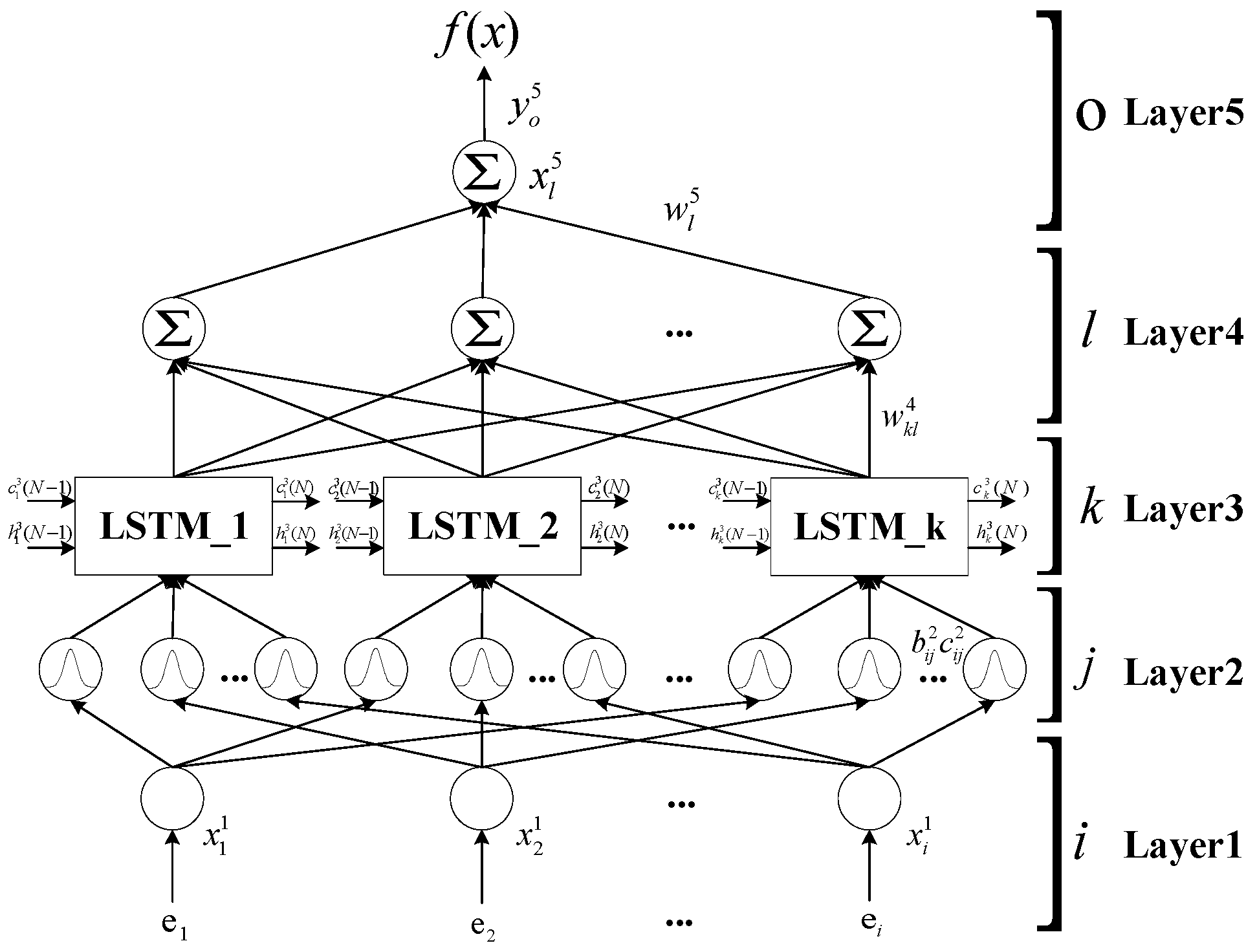
needs to be estimated. A novel FNN with an LSTM structure was adopted to identify the
, as shown in
Figure 1 and
Figure 2. Its unique recursive structure with LSTM greatly increased the ability to approximate unknown time-varying functions.
The basic rules and signal transmission of each layer of an NFNN are given in the following steps.
Layer 1—Input Layer: For node
of the input layer, the node input and output were derived as:
where superscript and subscript show the number of layer nodes respectively;
is the input,
are the network inputs,
is the output,
is a unity function of the
i-th node, respectively, and
N is the sampling iteration number.
Layer 2—Fuzzification Layer: The relationship in this layer is expressed as:
where
is the input of the fuzzification layer,
is the mean value,
is the standard deviation,
is the Gaussian function,
is the negative exponential function, and
is the output of the
j-th node, respectively.
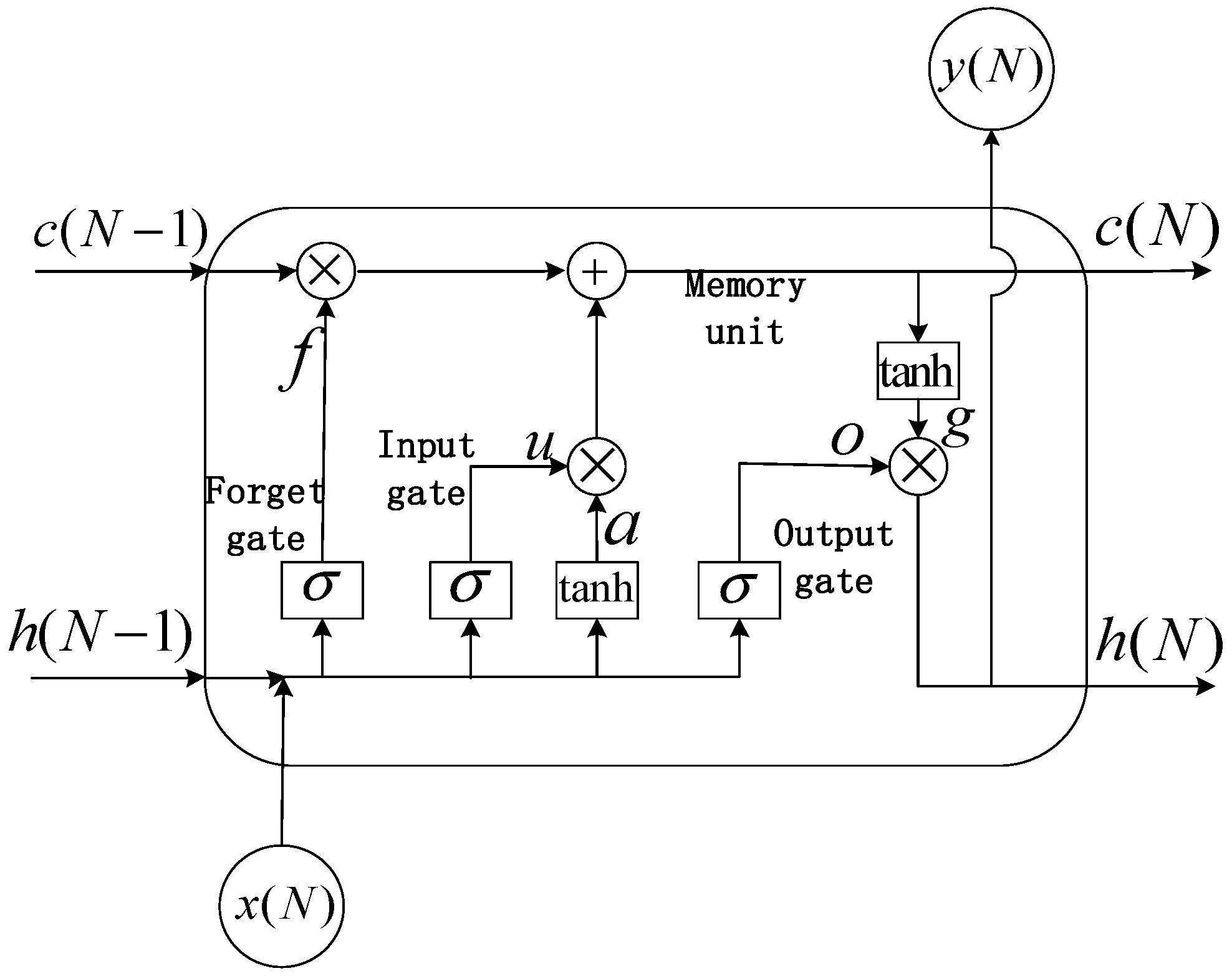
Layer 3—LSTM Layer: The relationship of this layer is expressed as follows:
where
where
,
,
,
are the weight and bias terms of the different LSTM parts, symbol
denotes dot product,
and
show nonlinear activation functions,
is the output of the forgetting gate,
is the output of the input gate,
is the state value,
is the output at the
N-th iteration of the
k-th node, and
is the output of the output gate.
Layer 4—Defuzzification Layer: The relationship of this layer is expressed as:
where
is the weight of the fourth layer’s
l-th node connected with the
k-th input,
is the network output, and
is the output of the
l-th node.
Layer 5—Output Layer: The relationship of this layer is expressed as:
where
is the weight related to the fifth layer output node and the
l-th input,
is the network output, and
is the final output.
The learning mechanism of the NFNN is summarized as follows:
- (1)
The system error is transmitted as the input to the fuzzy layer by the input layer.
- (2)
Then, each neuron of the fuzzy layer employs a Gaussian function to make the input fuzzified, and the output is then passed to the LSTM layer for information extraction and mining.
- (3)
The input of the LSTM layer and the feedback output of the previous state join with the input information channel and pass through three gates of forgetting, input, and output in turn.
- (4)
The output of the LSTM layer is then passed to the defuzzification layer, using the weighted average method.
- (5)
Finally, a weighted summation is accomplished on the defuzzification result to obtain the final output.
4. Adaptive Sliding Mode Controller Design Using the NFNN and Stability Analysis
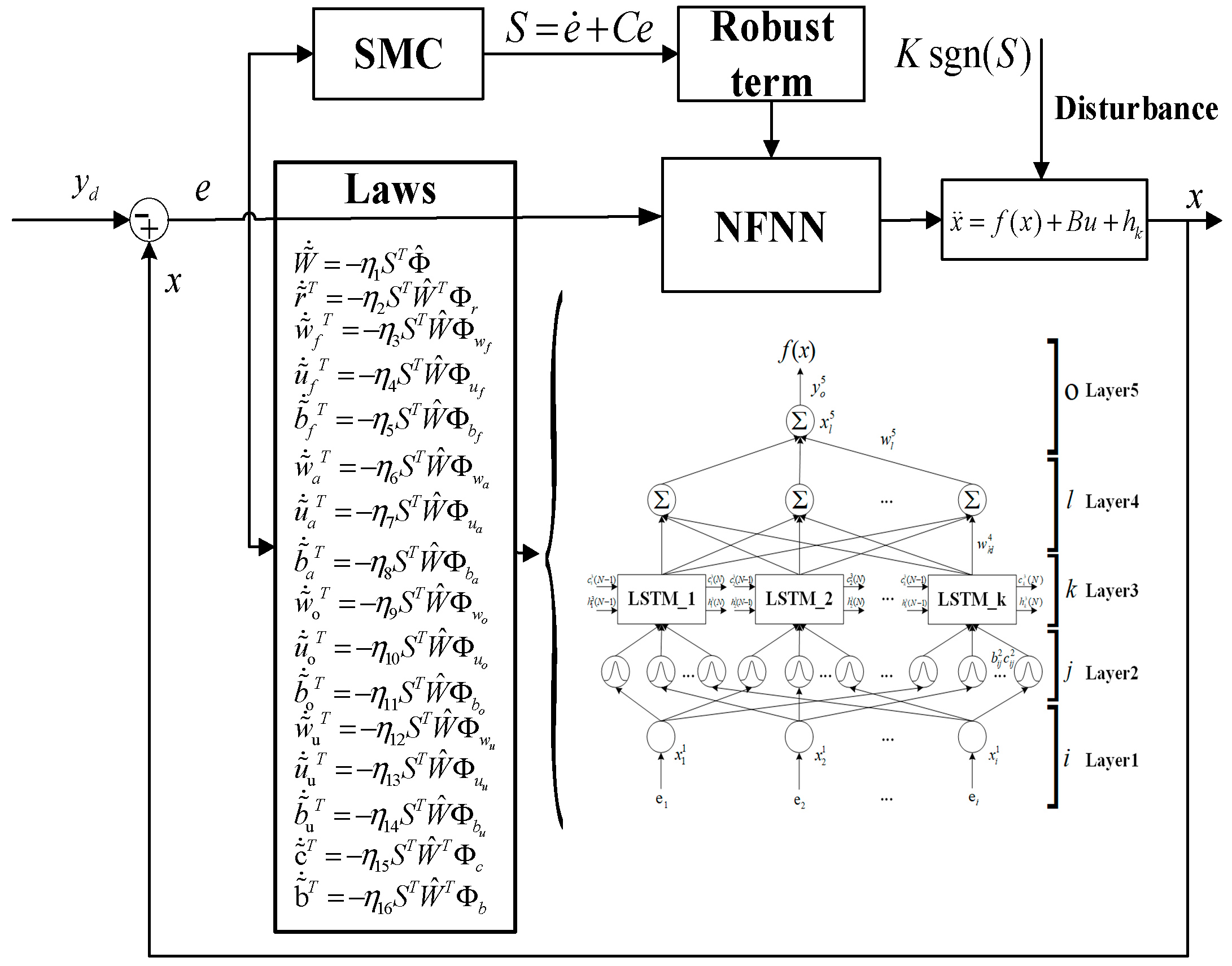
Figure 3 gives the block diagram of the designed ASMC-NFNN, which mainly includes three parts: reference signal, proposed controller, and dynamic system. In the controller module, the NFNN took the error information of the system as input, used the gradient descent method for optimization, and adaptively learnt in order to obtain the unknown uncertainty of the system; SMC as the main body of the controller, combined with the estimated value output by the NFNN and robust term, gave the final effective control law. In addition, the control object was a system that had unmodeled dynamics and was subject to internal parameter changes and external disturbances. The control goal was not to rely on an accurate system model to achieve the task of accurate control under different disturbances. The following introduces the design of the proposed NFNN and ASMC-NFNN controller.
According to the universal approximation rule, there are optimal weights to use the output of the NFNN to estimate any smooth nonlinear function. Consequently, a NN is designed to identify the unknown terms of the system.
Assume that optimal weights
,
,
,
,
,
,
,
,
,
,
,
,
,
,
,
exist that could estimate the unknown
. This five-layer NFNN is given in
Figure 1, written as:
where
,
,
is the ideal output in the fourth layer with regards to the weights,
is the ideal weight generated from online learning, and
is a reconstruction error, ensuring
,
is a positive value.
Practically, the estimate of
by the NFNN is written as:
Then, the estimation error of
function is derived as:
where
is the approximation error,
, and
. Then, the Taylor expansion of
is applied to convert the nonlinear NFNN into a partially linear form as follows:
where
is the higher-order term of the expansion and the partial terms, which can be calculated by the chain rule [
36], are represented as:
Then, from Equation (10), a practical controller is designed as follows:
Theorem 1. Considering the nonlinear system (4), the proposed controller with the ASMC-NFNN strategy can be guaranteed to be asymptotically stable if the following conditions are satisfied:
- (1)
The ASMC-NFNN controller is designed as in (41).
- (2)
The updating laws of the NFNN are derived as in (42)–(57).
whereare learning rate parameters, both of which are positive constants. Remark 3. Compared with the existing research, the proposed control strategy had a better control performance. First, compared to traditional sliding mode control, the ASMC-NFNN had the advantage of less chattering because, in the case of unknown system disturbances, traditional sliding mode control often relies on high-gain switching gain to achieve disturbance compensation. Although this could bring a good steady-state performance, it could cause high-frequency output chattering, which could bring huge adverse effects to the system. On the contrary, the proposed method firstly relied on the learning and estimation ability of the neural network to realize the active compensation of the disturbance, thereby reducing the burden of the sliding mode on the disturbance, and reducing the system chattering while improving the performance. Second, the proposed strategy had better dynamic performance and robustness than other neural network-based sliding mode control strategies because it adopted a novel neural network with an LSTM structure. As mentioned above, in theory, it had a selective forgetting mechanism, avoided the problem of gradient disappearance, and had the advantages of a strong learning ability. Therefore, it could compensate for the unknown time-varying uncertainty of the system faster and more accurately, and, thus, had better dynamic performance. The subsequent simulation comparison results also showed that the proposed control strategy could cope with larger parameter changes and had better dynamic performance.
Proof. The following Lyapunov function is designed as:
where
is positive definite. The last 16 items in Equation (58) are denoted as
. □
Remark 4. The designed Lyapunov function not only included the quadratic form of the systematic error, but also the quadratic form of the estimation error of the neural network weight, which not only ensured the convergence of the systematic error, but also ensured that the parameter error was small. In addition, because the learning rate of the weight was relatively large, the quadratic term of the system error had a larger proportional coefficient than the weight error, which meant that the convergence of the system error was guaranteed to a greater extent. In addition, compared with the traditional neural network method using gradient descent to optimize the error, this paper incorporated the quadratic form of the weight error into the design of the Lyapunov function, so that the adaptive rate of the neural network could be reversely derived through the stability proof. Although the form of the two was found to be similar after derivation, it was clear that the method proposed in this paper had more theoretical support, which was a unique contribution of this paper.
Taking the derivative of (58) and then substituting (8) into it the following is obtained:
Substituting Taylor’s expansion (40) into (59) yields
Finally, substituting the updating laws (42)~(57) into (60) the following is obtained:
where
. Suppose
and
have upper bounds
and
respectively as
,
. So, if
,
.
Because is a semi-negative definite, , are bounded. From inequality , is integrated as . is bounded and , is bounded. From Barbalat’s lemma, and asymptotically converge to zero as .
5. Simulation Study
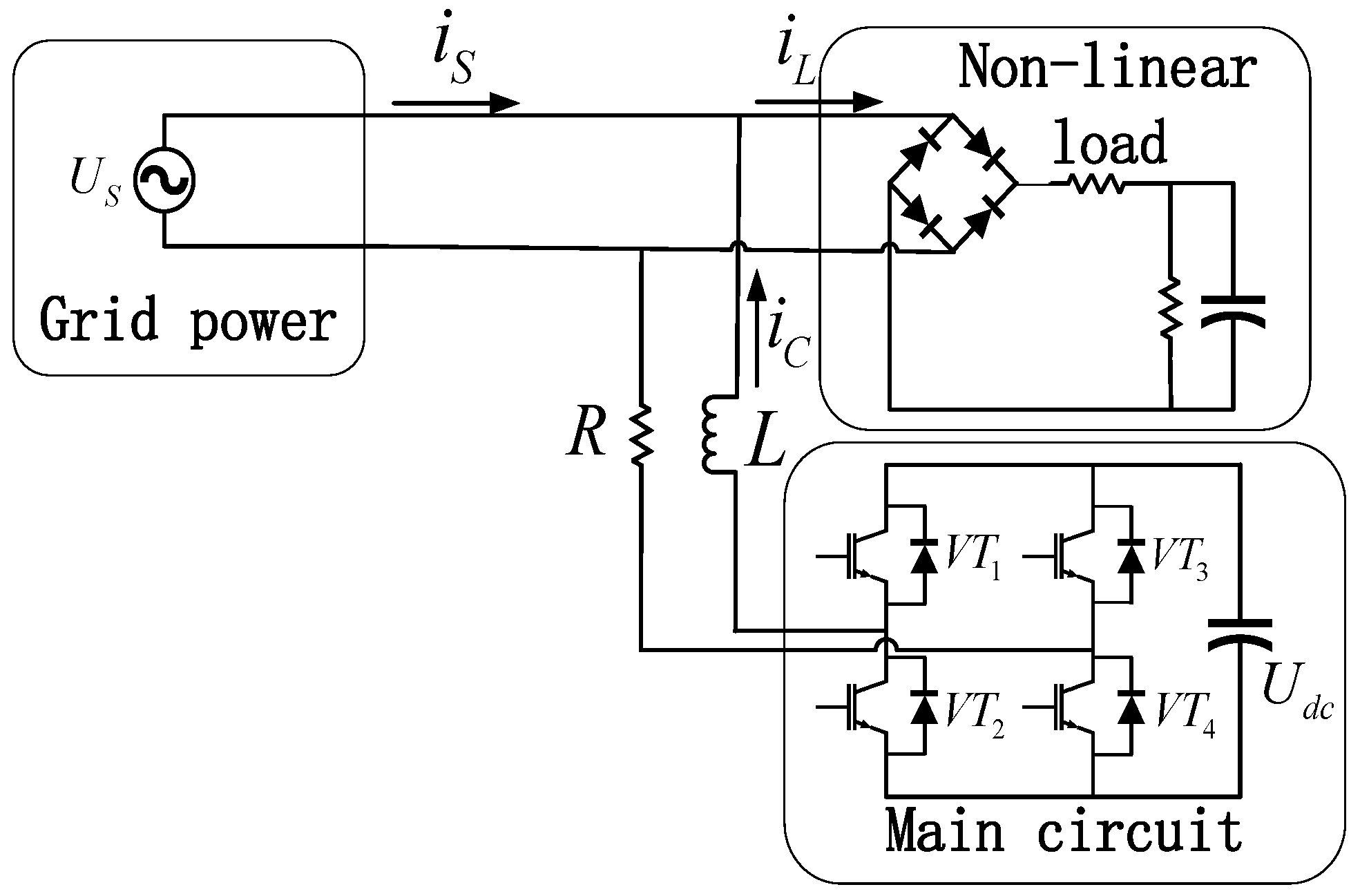
To verify the effectiveness of the proposed ASMC-NFNN algorithm, a simulation experiment was performed using Matlab/Simulink with a single-phase active power filter (APF), as in
Figure 4. In the simulation experiment, the computer system was 64-bit, the CPU was i7-6500 U (2.5 GHz), and the Matlab software version was 2019b. The shunt single-phase APF circuit model had three main components: grid voltage, nonlinear load, and APF main circuit.
In fact, the APF controller included three parts: harmonic detection module, DC side voltage control module, and compensation current tracking control module. The control goal was to force the compensation current to follow the reference current quickly and accurately. On the one hand, the harmonic detection module was implemented by a single-phase fast harmonic detection algorithm, which could obtain the reference current in real time. On the other hand, the control of DC side voltage was realized by traditional PID control due to low control requirements and low control difficulty, and voltage stability was achieved by superimposing the output of the PID controller into the reference information. Therefore, the voltage on the DC side was stable and could be regarded as a constant.
From circuit theory, the following equations are obtained:
where
is a grid voltage,
is a compensation current,
is a capacitor voltage in DC side, and
L and
R are inductance and resistance. respectively.
is defined as
In this paper, the state equation for the compensation current was studied since a PID controller applied in the DC side voltage made it easy to obtain the voltage requirements. The compensation current is derived as
However, under system uncertainties and disturbances, the state equation for the compensation current is further revised as
where
and
are the uncertainties of
R and
L respectively, and
is the other uncertain component. Further, Equation (65) is rewritten as:
where
is the lumped uncertainty bounded by
, as
.
Taking the derivative of Equation (66) one gets
Then, the second-order dynamic equation is obtained as:
where
represents
,
represents
, which is a known constant,
represents
, which is an unknown function whose exact value is difficult to obtain,
represents
, and
is the lumped uncertainty, with an upper bound
, as
.
The parameters in the system simulation are explained in
Table 1. The parameters of the PID controller and the ASMC-NFNN controller are given as
In the NFNN, learning rates were , the initial values of the center and width in Gaussian function were selected as , , and the initial weights were chosen to be 1, except for the initial weights in the fourth layer and in the fifth layer.
Simulation verification included three aspects: (1) steady state response simulation for harmonic compensation; (2) dynamic response simulation and comparison with recurrent FNN; (3) parameter variations simulation and comparison.
5.1. Steady−State Response
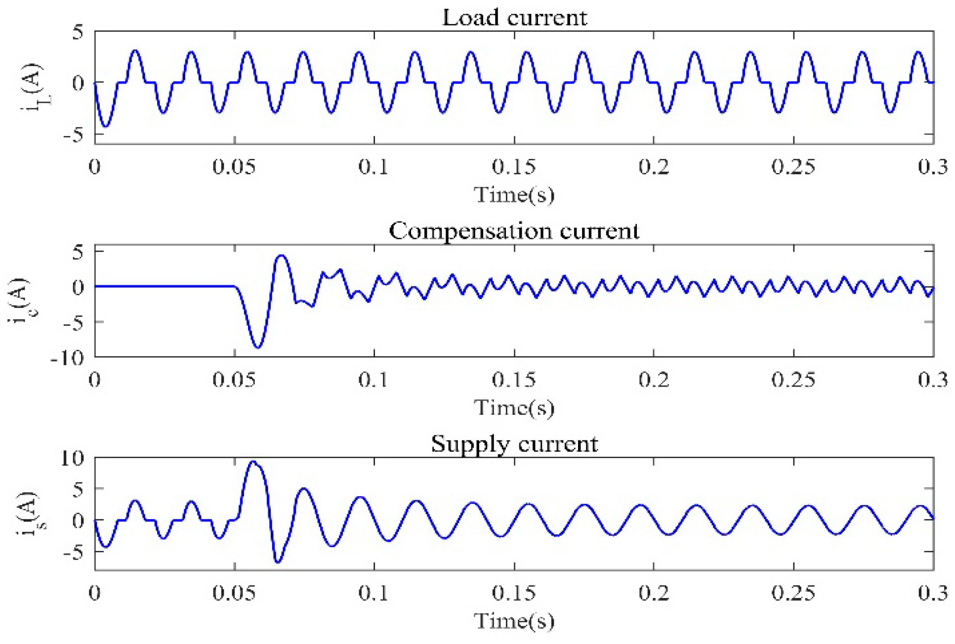
In the simulation, the harmonic compensation was set to be added in the APF system from 0.05 s.
Figure 5 gives the steady-state response of the system under the proposed ASMC−NFNN. The waveform diagrams were load current, power supply current, compensation current tracking curve, and tracking error figure, in order. As can be seen from the load current curve in
Figure 5, the load had serious nonlinear distortion and caused serious harmonic distortion in the power supply current.
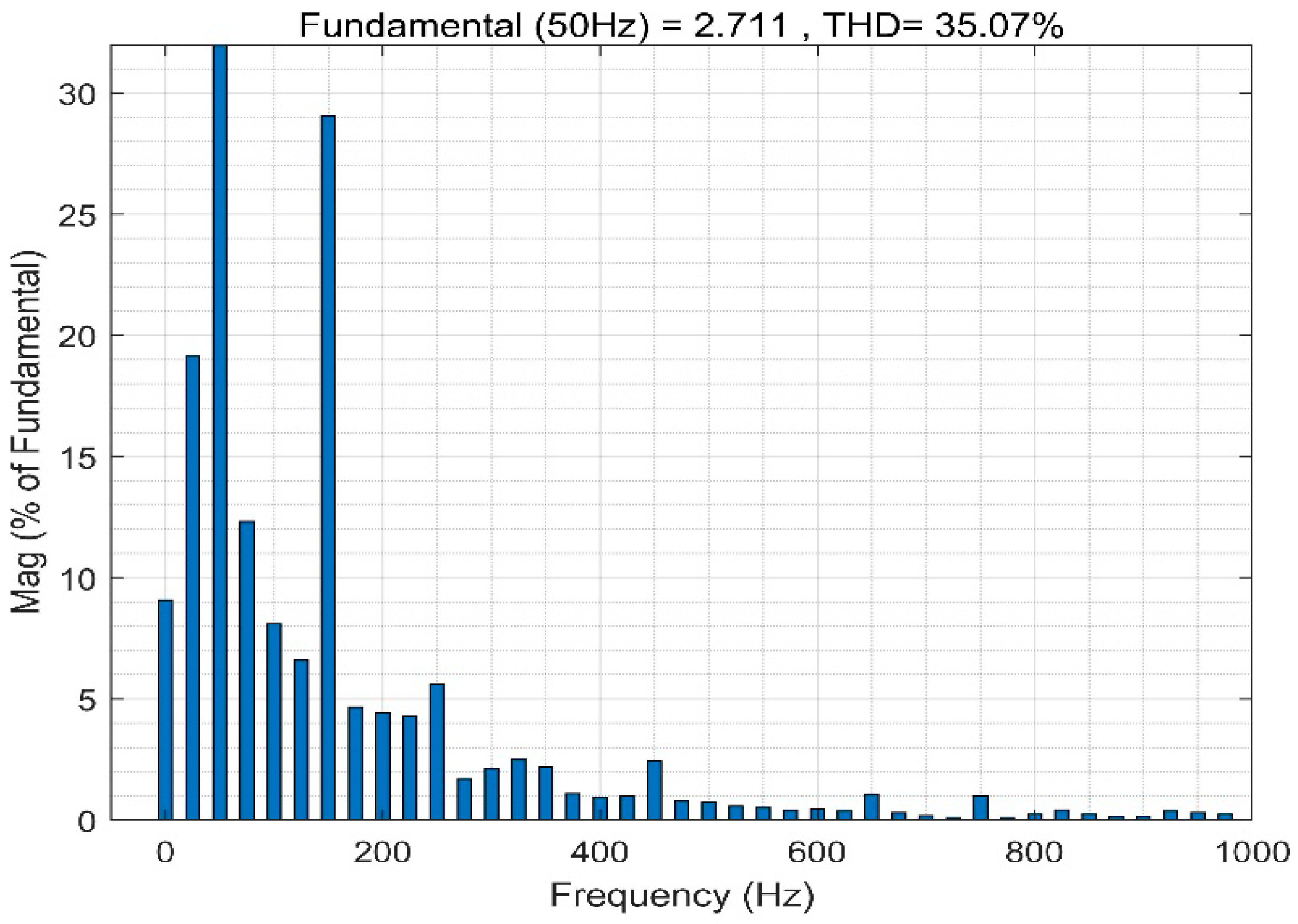
The degree of harmonic distortion could be seen from the spectrum analysis chart in
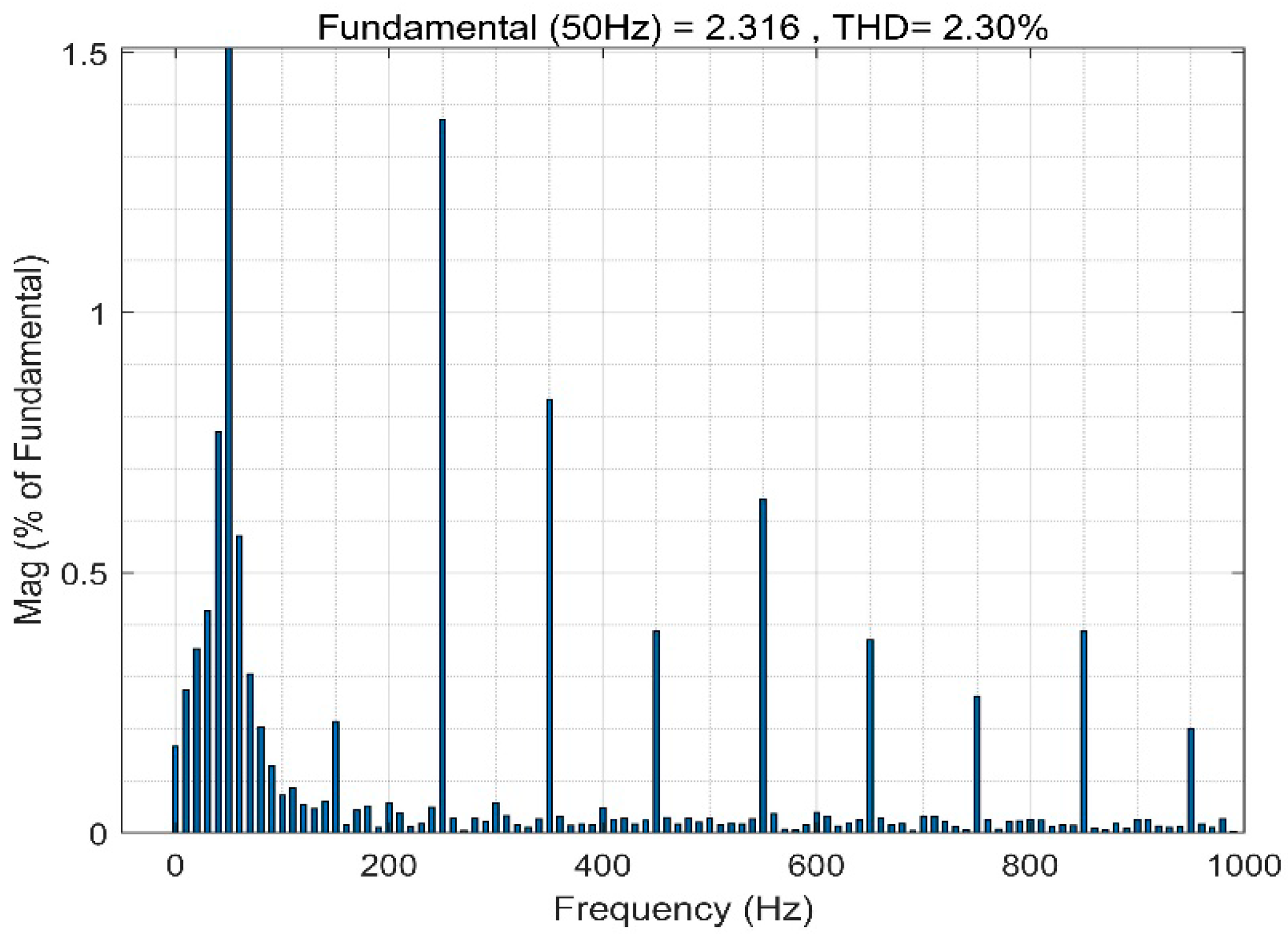
Figure 6. In addition to the fundamental wave, there were many harmonics, and the total harmonic distortion (THD) rate reached 35.07%. However, after APF started to control at 0.05 s, the harmonics were suppressed in a short time. From
Figure 7, the THD was reduced to 2.3%. Therefore, APF using the ASMC−NFNN controller could well purify harmonic pollution. As shown in
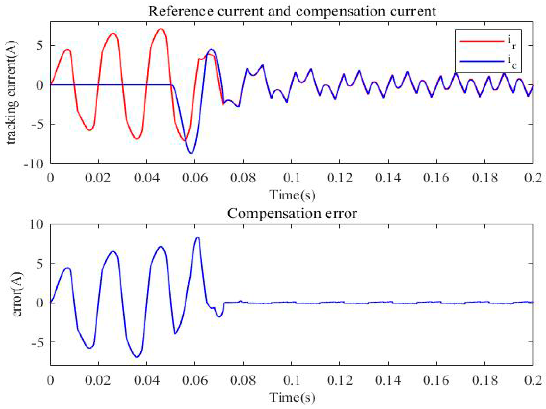
Figure 8, the compensation current curve and the reference current curve almost completely coincided after a short time, and the tracking error was also nearly zero, which reflected the high accuracy of current tracking, fast response, and good harmonic compensation effect.
Figure 9,
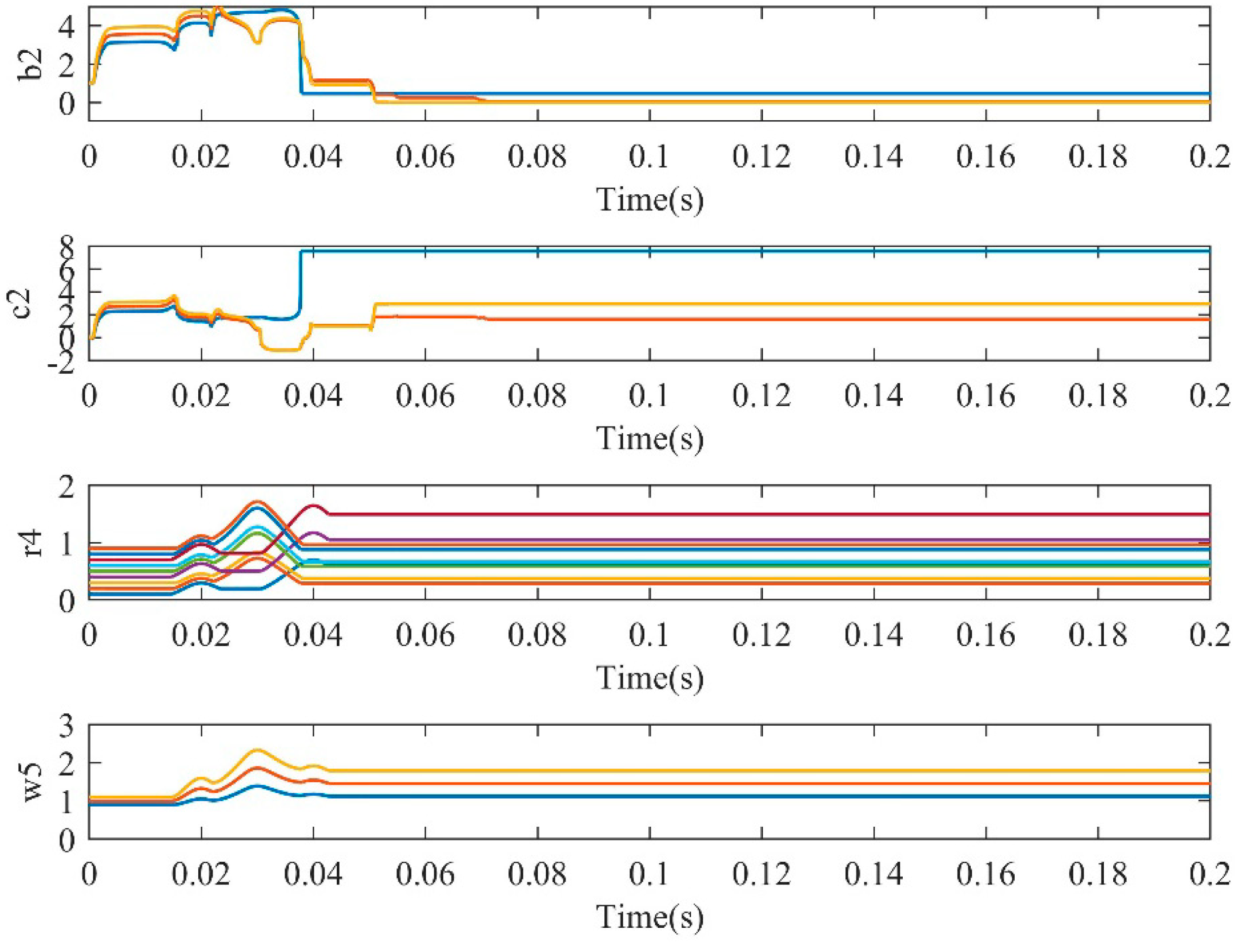
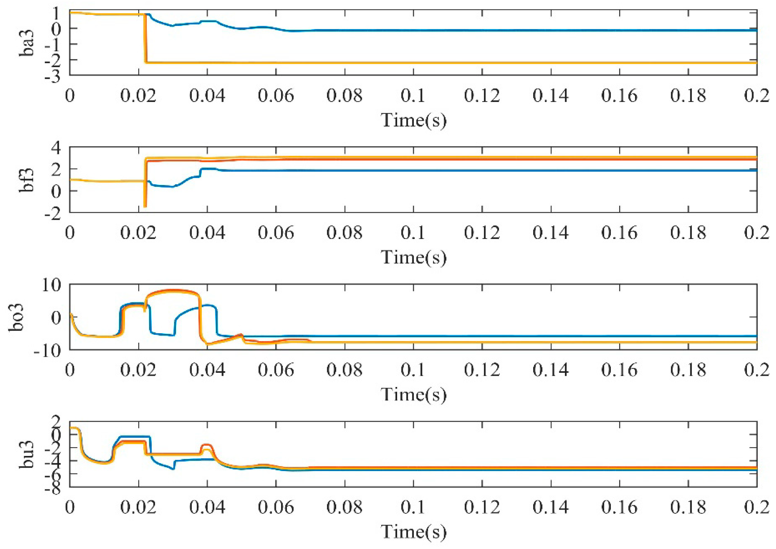
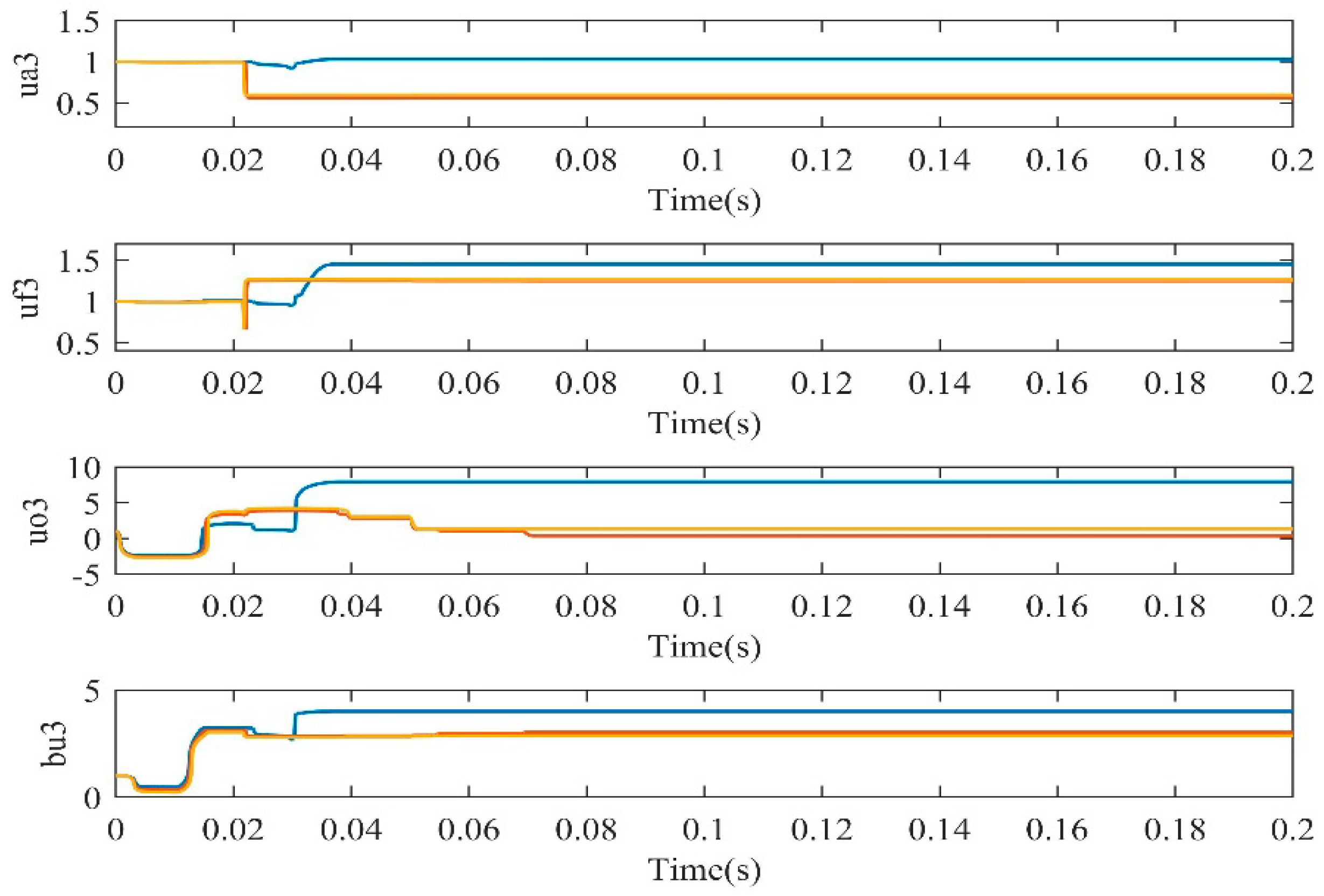
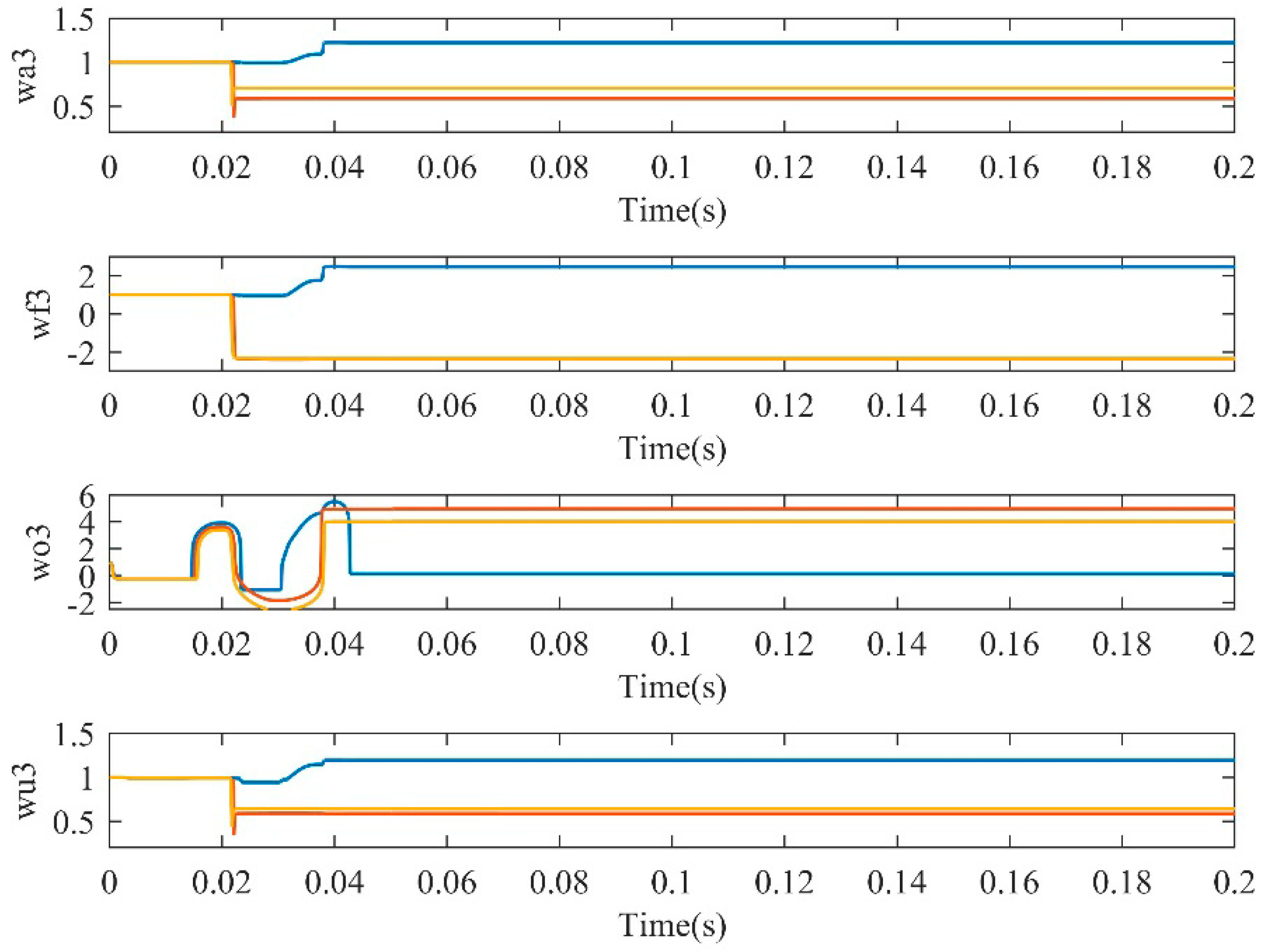
Figure 10,
Figure 11 and
Figure 12 give adaptive adjustment curves of some parameters of the NFNN, which did not need to be adjusted manually. After adaptive learning, convergence was achieved in a short time and the system response could also achieve good results. This showed that the NFNN had an excellent adaptive adjustment performance and stability.
5.2. Dynamic Response Simulation and Comparison
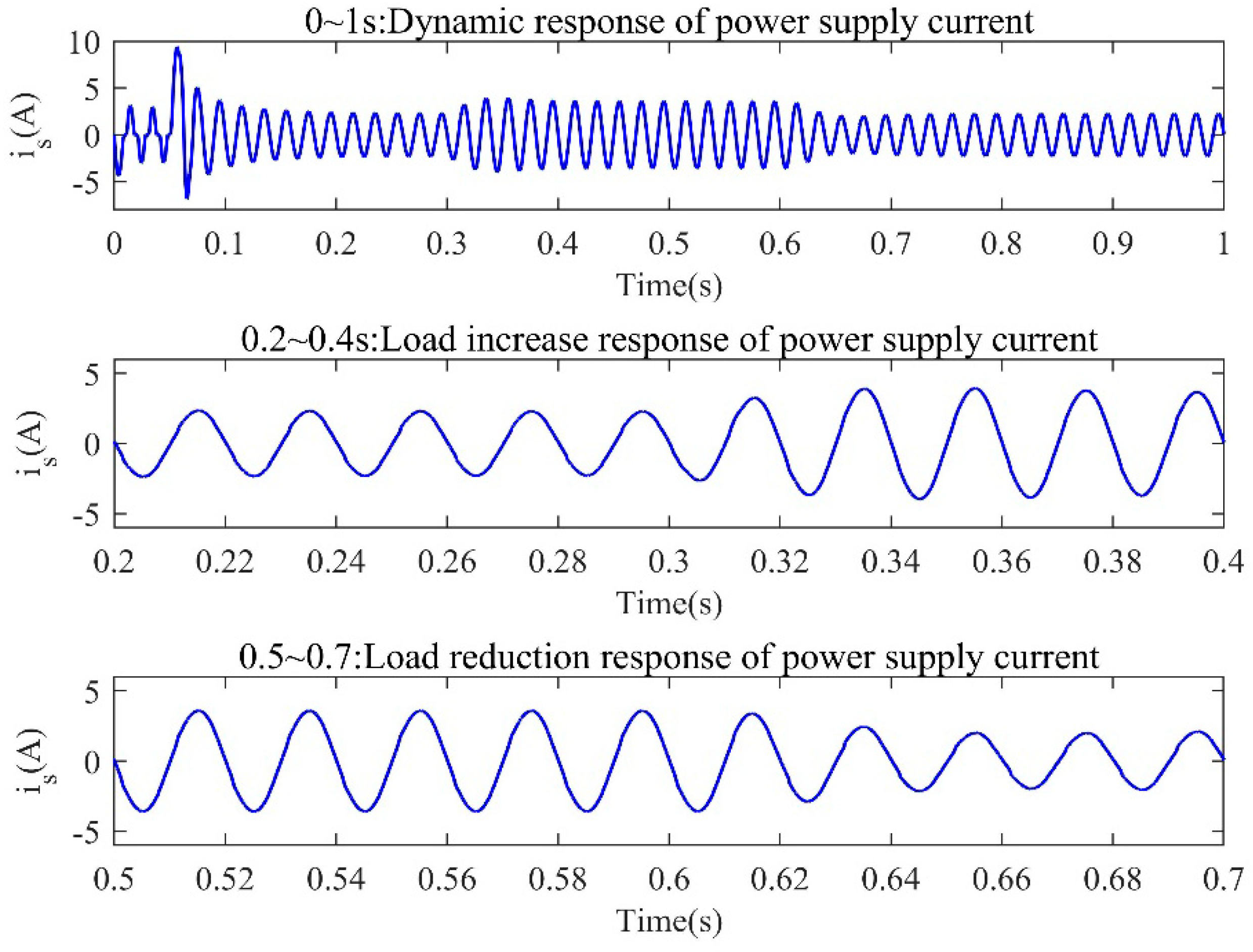
To verify the ability of APF to compensate for harmonics under sudden load changes using ASMC−NFNN, sudden load increase and decrease experiments were designed and the comparison simulation with ASMC−RFNN was given.
In the dynamic simulation, the APF was connected to the system at 0.05 s, and a nonlinear load was added at 0.3 s and subtracted at 0.6 s. In addition, the parameters of the increased load are given in
Table 1. The dynamic response of the APF system was observed when the load changed. The dynamic response waveforms of the supply current using ASMC−NFNN is shown in
Figure 13, which shows that no matter when the load was increased in 0.3 s or the load was decreased in 0.6 s, the power current returned to a sinusoidal steady state after a short adjustment, showing that the proposed controller worked well under load changes with good dynamic properties.
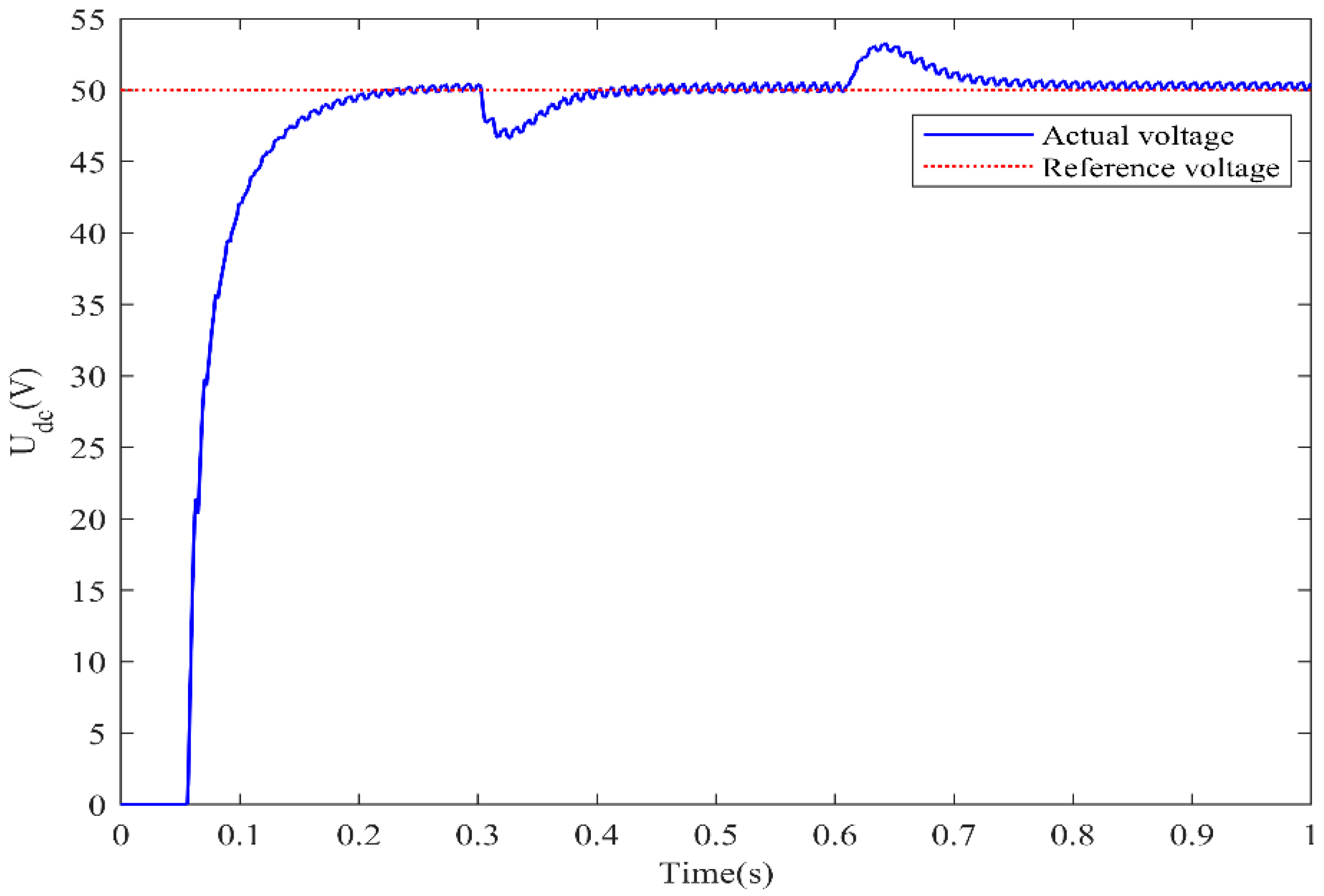
Moreover, the voltage control curve on the DC side is shown in
Figure 14, verifying the previous assumption that the DC side voltage was stable.
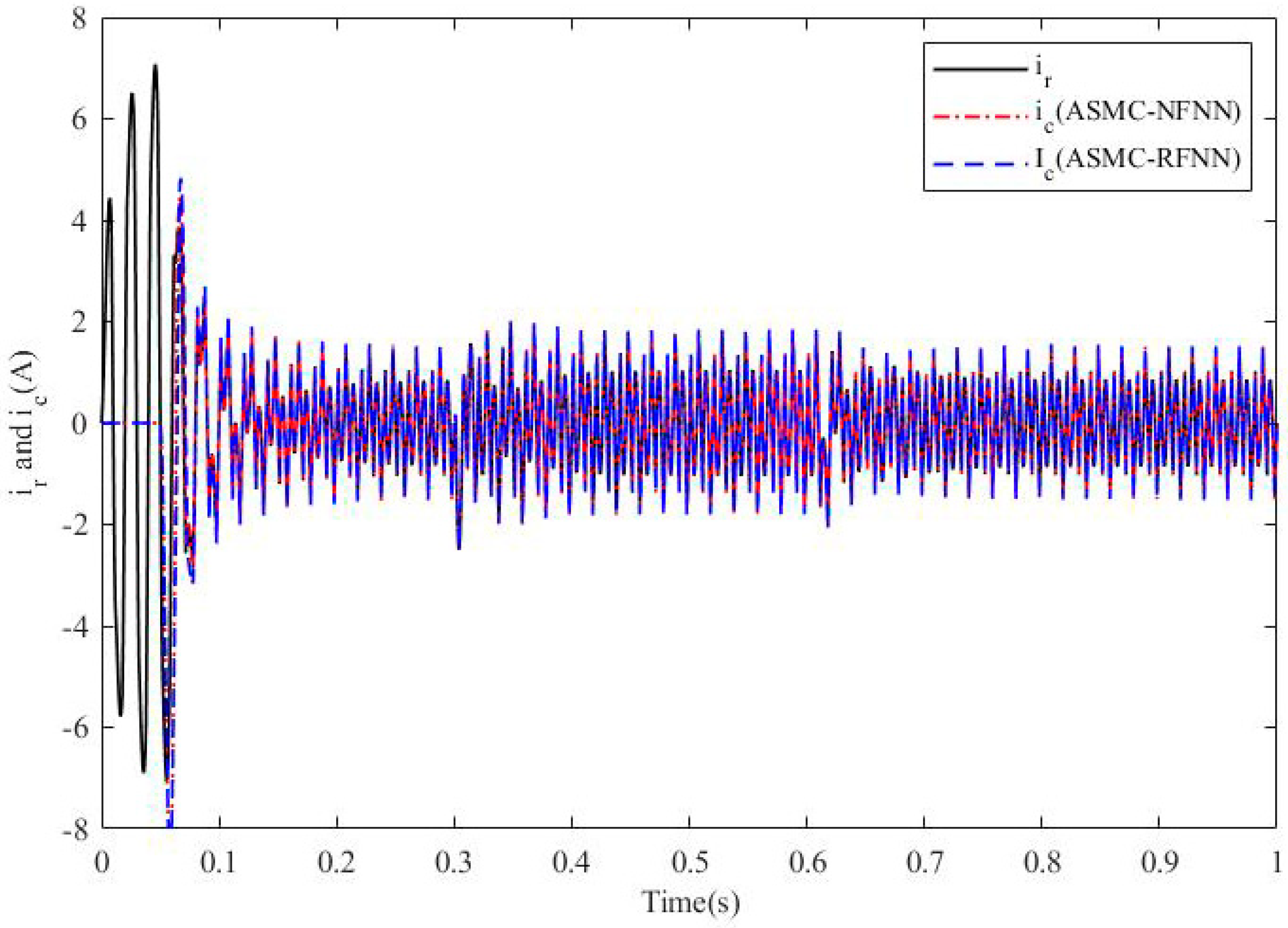
Moreover,
Figure 15 shows the current tracking curves under the two methods. In both methods, the compensation current could track the reference current when the load changed. Moreover, it was roughly seen that the tracking curve of the comparison method was over-tracked and covered other curves, so its tracking compensation performance was worse.
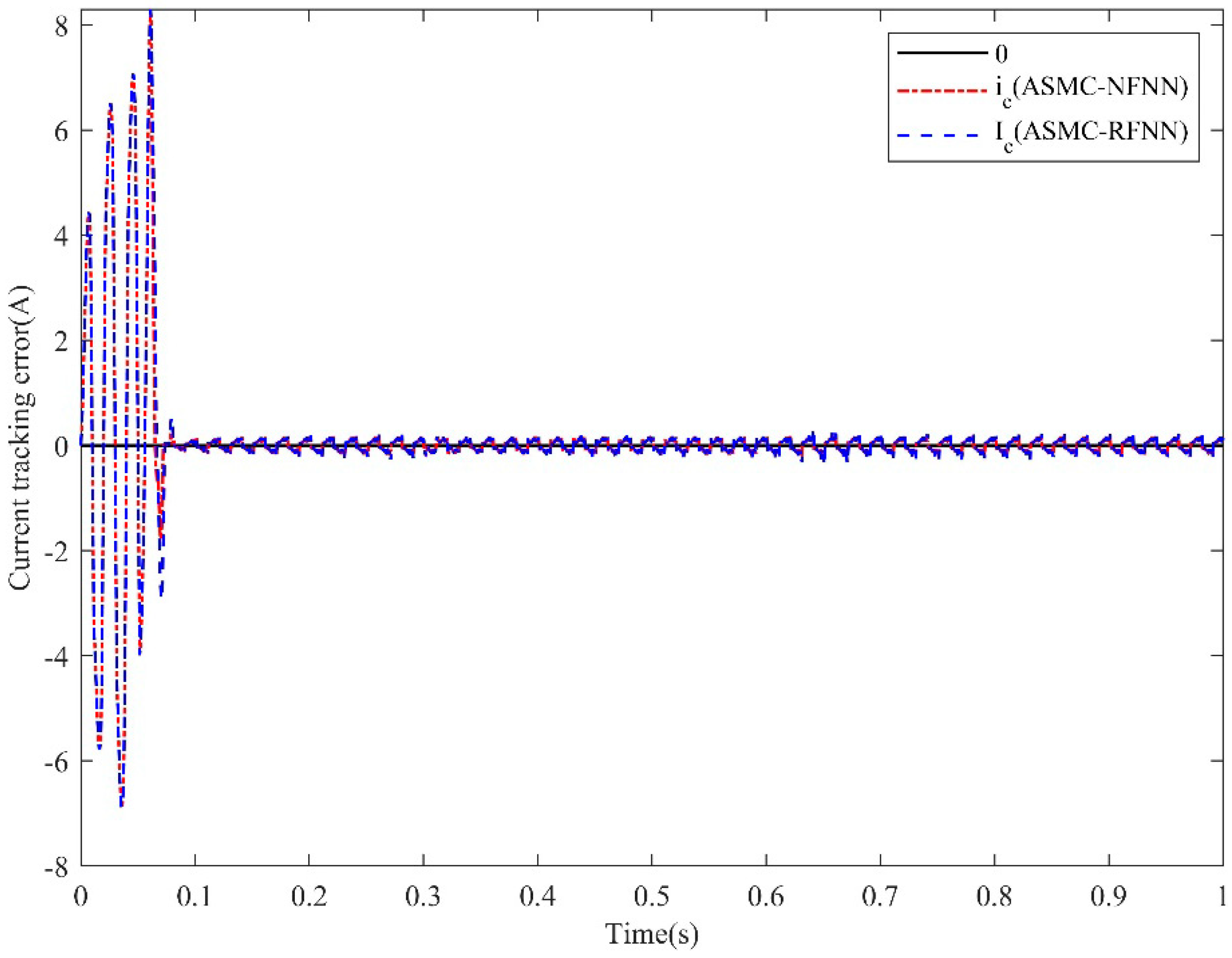
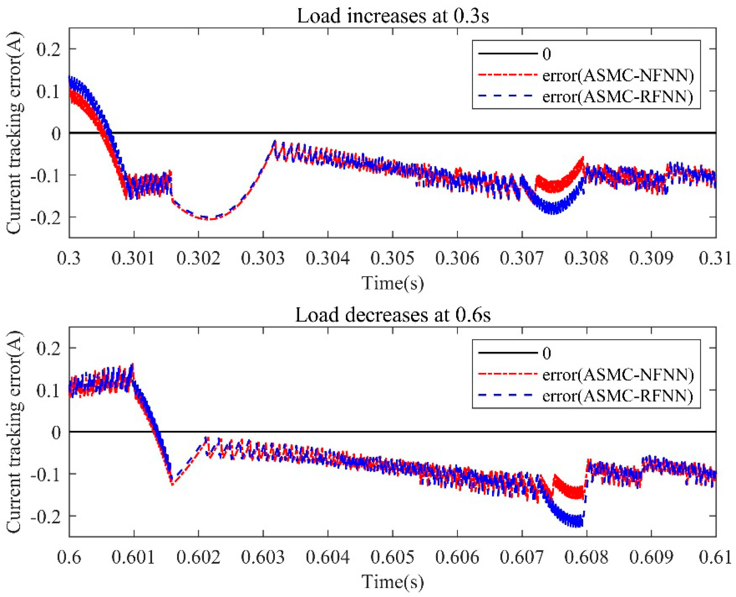
In order to see a more obvious comparison, the overall tracking error comparison curves are given in
Figure 16, and the partial enlarged comparison curves at the load change point are given in
Figure 17. It was clearly seen from
Figure 17 that the error of the proposed method (red curve) at the two load change nodes was closer to 0 than the comparison method (blue curve). Therefore, the proposed controller with NFNN had better dynamic performance than the RFNN.
Several performance indicators were used to analyze the proposed NFNN-based controller and the comparative RFNN−based controller. The performance comparison results of THD are shown in
Table 2. In three experimental states, the ASMC-NFNN had a smaller THD than the ASMC−RFNN. In addition, compared with the dynamic terminal sliding mode controller using a double hidden layer recurrent neural network (DTSMC−DHLRNN) proposed in Ref. [
40], the THD performance of ASMC−NFNN in steady state was 0.66% better. In addition, the comparison results of some commonly used performance indicators are given in
Table 3, showing the proposed controller was superior to the comparison method in various error performance indicators. However, in the indicator of simulation calculation time, because the proposed method had a more complicated structure, the calculation time was slightly longer than the comparison method. In fact, the update complexity per weight and time step of the LSTM algorithm was, essentially, that of BPTT, namely O(1), and LSTM was local in both space and time [
36]. Therefore, the extra complexity introduced by LSTM was not high and, fortunately, with the upgrade in computing power, the subtle difference in computing time was no longer a serious problem.
5.3. Parameter Variations Simulation and Comparison
Practically, it was not easy to obtain accurate parameters of the controlled object, especially in the power system occasions, as the component parameters would also dynamically change. For example, the aging of the resistance made the resistance value larger, and the inductance would change subject to environmental factors, such as temperature and magnetic field. The changes in the internal parameters of these systems were called internal disturbances, which would make the performance of general controllers worse and even difficult to use in practice. Therefore, this section studies the robustness of the proposed controller under parameter changes and compares it with the other two methods. The selected variable parameters were the resistance and inductance values on the APF main circuit.
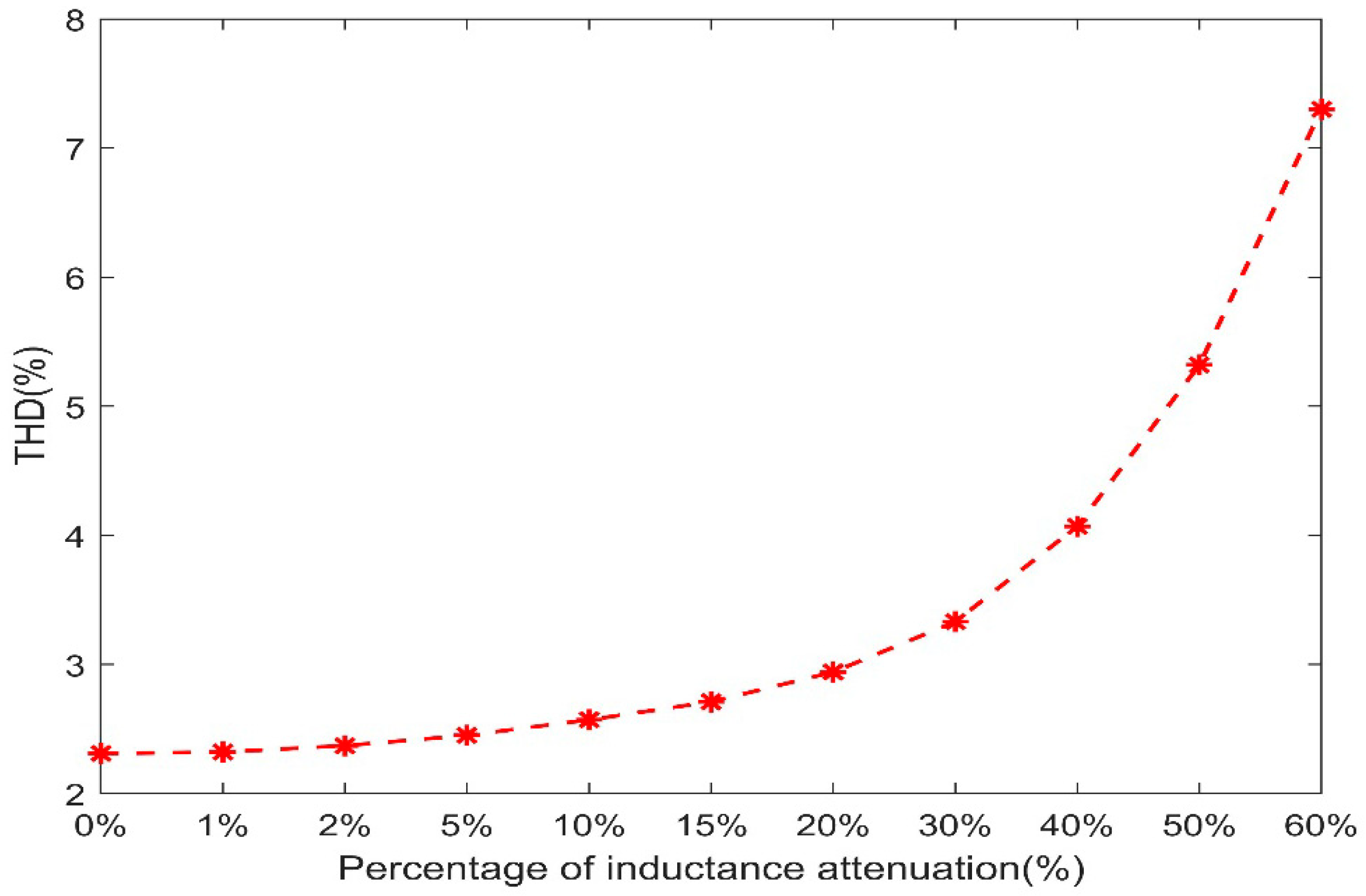
Figure 18 shows the change curve using ASMC−NFNN of the steady−state THD value with different degrees of inductance attenuation. When the inductance attenuation percentage was small, the THD hardly changed. When the inductance attenuation degree gradually became larger, the value and the change range of THD also increased continuously. This showed that the inductance parameter had a great influence on the system performance. However, it could be seen from the figure that even if the inductance was attenuated by 40%, the THD of the power supply current was still below 5% under the proposed method, which could still meet the application requirements. Therefore, the proposed method had a large tolerance space for inductance parameters, and had good robustness in terms of inductance parameter changes.
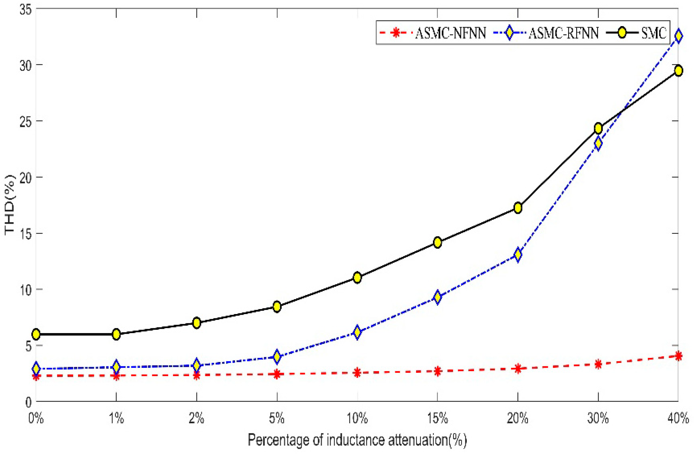
In addition, the steady−state THD comparison chart of the three methods under inductance attenuation is given in
Figure 19, showing that the proposed strategy had the smallest THD variation and the best parameter tolerance. The method based on ASMC−RFNN had a small THD change when the inductance attenuation was small; when the inductance attenuation was greater than 5%, the THD increased sharply; after the inductance attenuation was 30%, the THD even exceeded the ordinary sliding mode controller. The above shows that when the inductance attenuation was greater than 30%, the RFNN network of the ASMC-RFNN method fell into disorder and failed to learn the system parameters correctly. At the same time, it proved that the NFNN had a better learning ability and adaptability than the RFNN. On the other hand, when the inductance parameters were not particularly large, the proposed algorithm with the NN had greater tolerance to inductance parameters and a smaller THD change trend than ordinary sliding mode controllers, showing the advantage of good robustness.
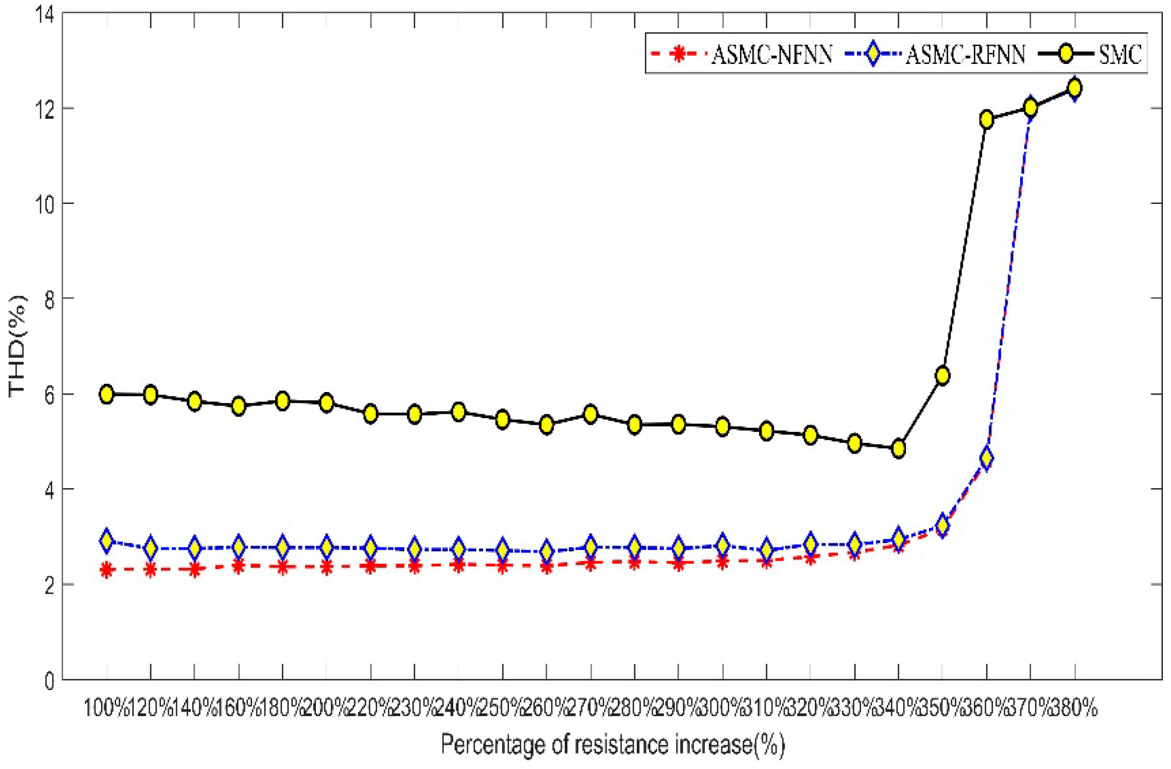
At the same time, the simulation comparison chart of resistance variation is given in
Figure 20, showing the change in the resistance had a very small effect on the system performance. The SMC−based method could tolerate an increase of 3.4 times in resistance, while the proposed ASMC−NFNN could tolerate an increase of 3.6 times in resistance. In general, changes in resistance parameters had a limited impact on the system, and ASMC−NFNN methods had better performances, to some extent.
6. Conclusions
In this paper, an ASMC-NFNN strategy was studied for a general class of dynamic systems with unknown uncertainties. Considering the existence of time-varying unknown uncertainty perturbations in such systems, an NFNN with an LSTM structure was developed to approximate the system uncertainty where the LSTM structure had a special gating unit that could selectively forget and remember, which was suitable for long-term dependent learning problems. In addition, a sliding mode controller was given to implement the tracking control of nonlinear systems, ensuring high tracking accuracy and fast response speed under estimation error and external disturbances. An NFNN online learning algorithm was derived and all the parameters of the NFNN were guaranteed to converge under the adaptive laws. The proposed control strategy were verified on the second-order single-phase APF system, and the numerical experimental results showed that it had better steady-state and dynamic properties than other control methods, and also had better robustness in the presence of parameter changes. Considering that the control strategy was universally designed, and the algorithm integrating neural network and sliding mode were very suitable for power electronic control, the strategy could be extended to the control of a series of similar electronic power systems, and could achieve superior results. In future research, reducing the computational complexity of neural networks and the difficulty of parameter adjustment will be a hot research direction. In addition, the use of more advanced adaptive super-twisting sliding modes is also expected to be a promising research direction.


