
New Result for the Analysis of Katugampola Fractional-Order Systems—Application to Identification Problems

 and
and 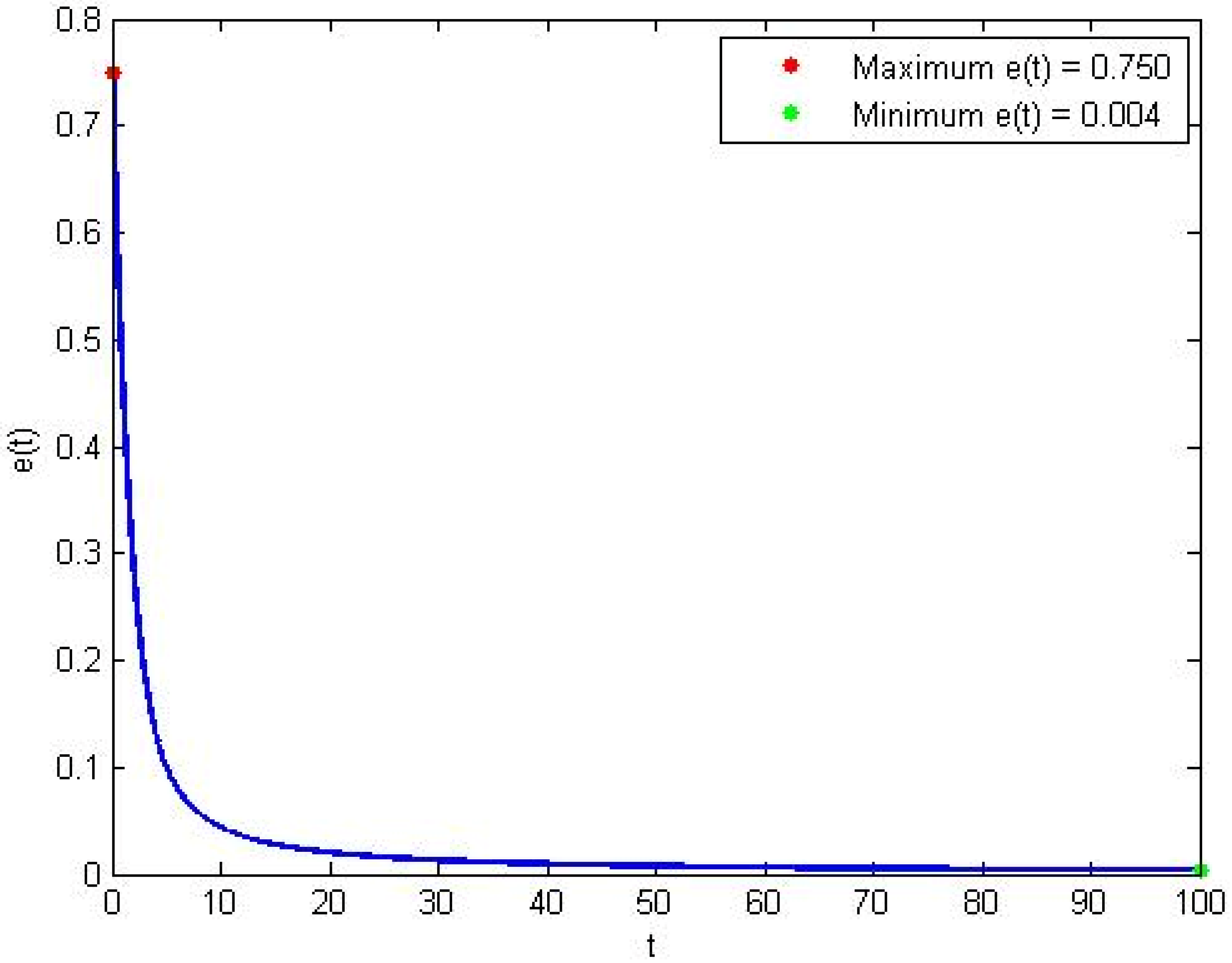
Abstract
:1. Introduction
- The main novelty in this work was that it presents a new Barbalat-like lemma for the class of Katugampola fractional-order systems. To the knowledge of the authors, such a particular result is developed for the first time, and no existing papers have demonstrated it.
- In a second stage, the authors exploited this new lemma in two identification schemes. In the first scheme, a Fractional Error Model 1 was investigated to the class of Katugampola fractional systems. In the second scheme, two adaptive Katugampola fractional systems, related by a linear constraint, were considered. In this case, the so-called “Fractional Error Model 1 with parameter constraints” was used.
2. Preliminaries
3. Evolution of a Function with a Bounded Katugampola Fractional Integral
- (i)
- If , then :ThenThen, by using (3), one can find
- (ii)
- If , then :ThenThen, by using (3), one can findThen
4. Application to Identification Problems
4.1. Identification Using Fractional Error Model 1
4.1.1. Theoretical Study
- : In this case, (9) reduces to the convergence in mean value of :
- : This case corresponds to the classical Caputo derivative concept. An analogue study has been conducted for Caputo fractional systems, in [22].
- and : This case corresponds to the integer-order calculus framework. In this case, the adaptive law is (6), instead of (7). Moreover, from a theoretical point of view, (9) reduces to the convergence to zero of .
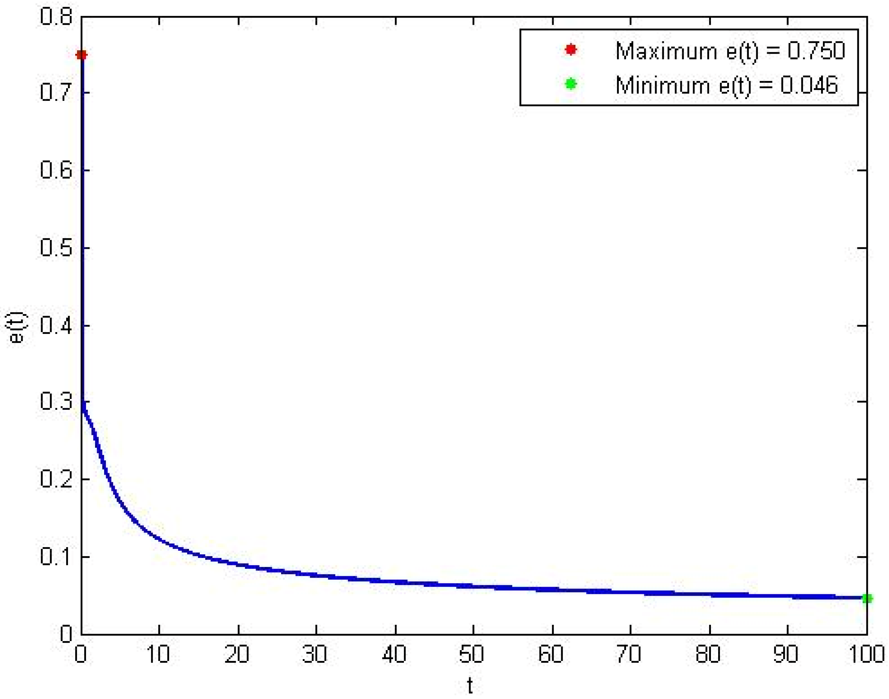
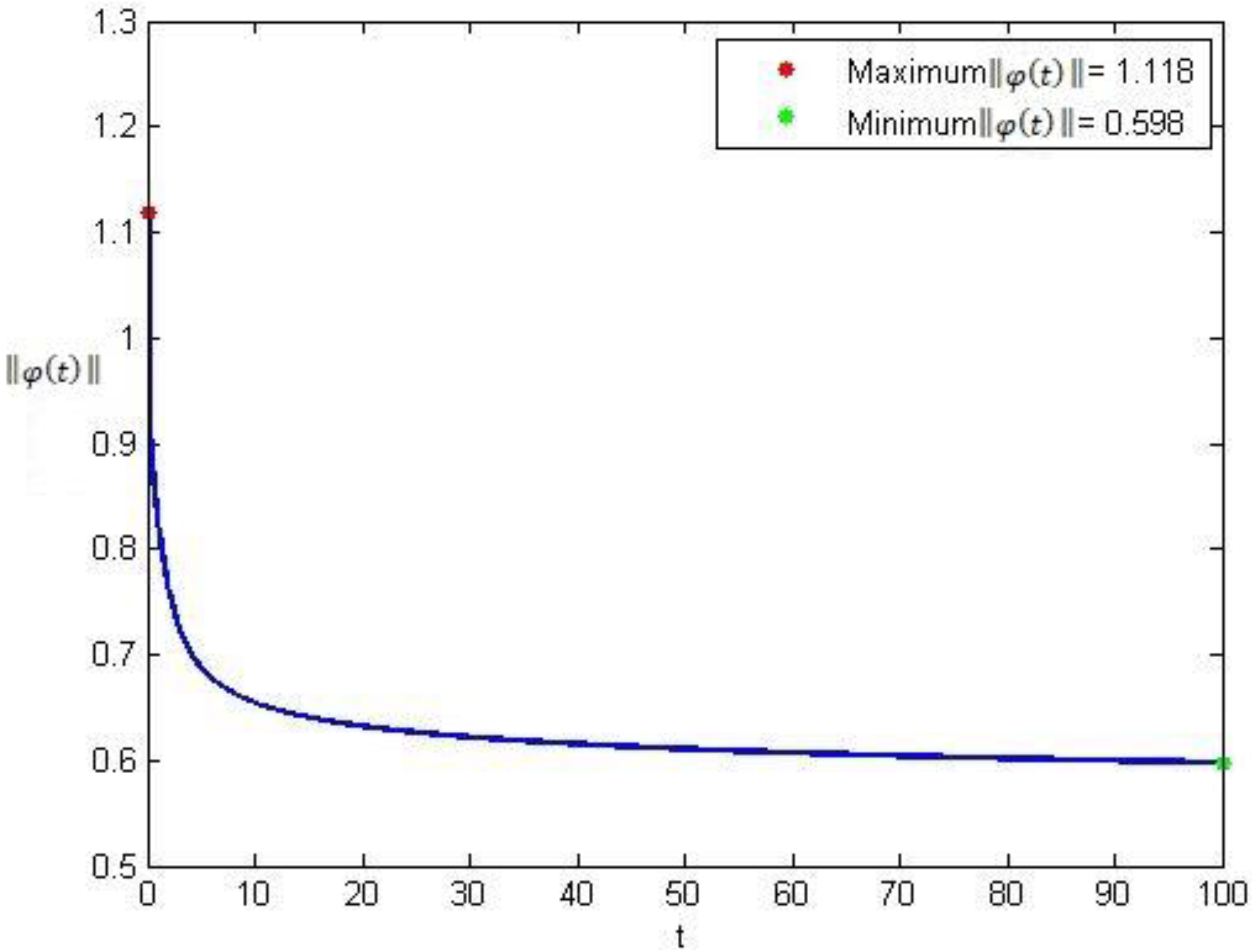
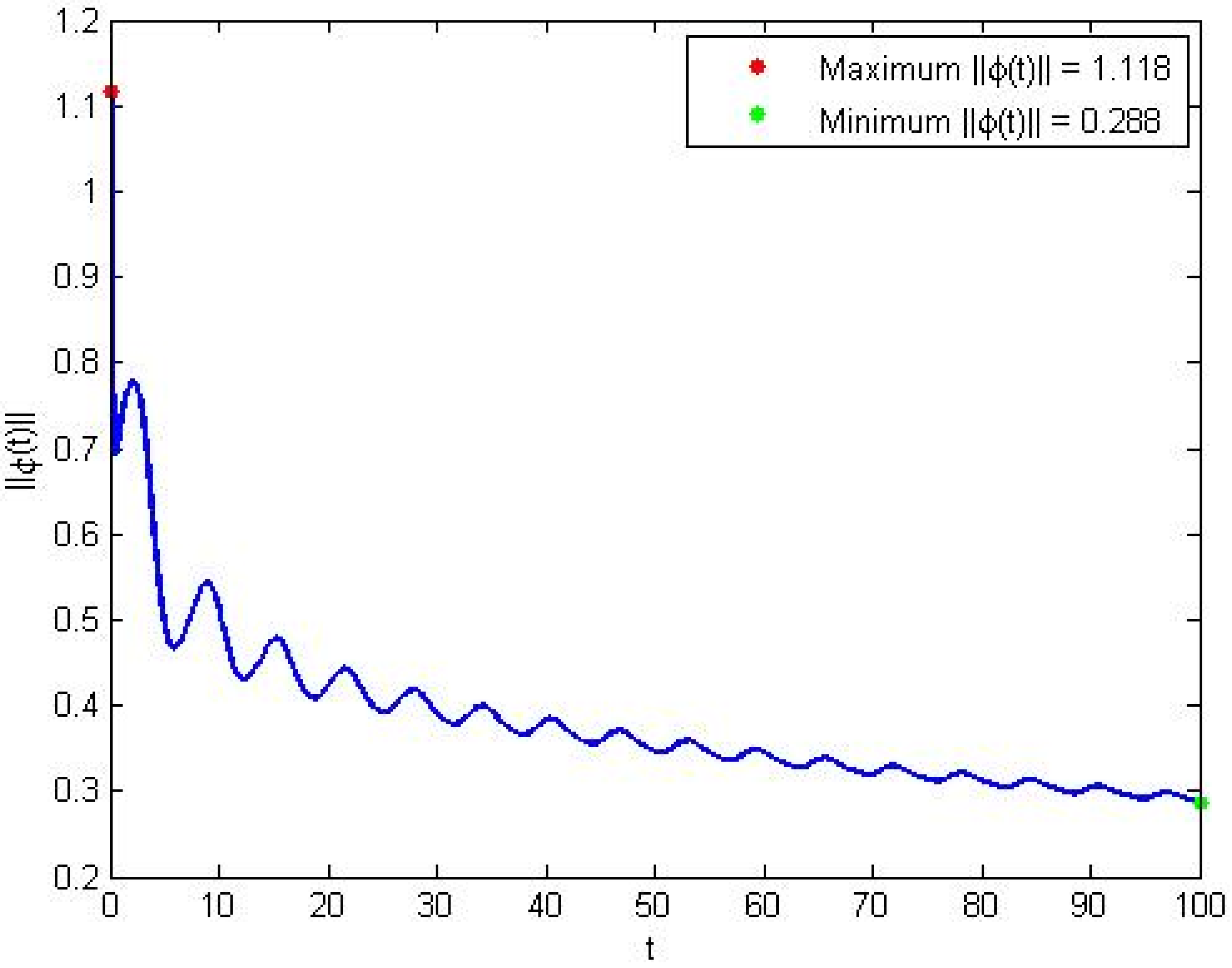
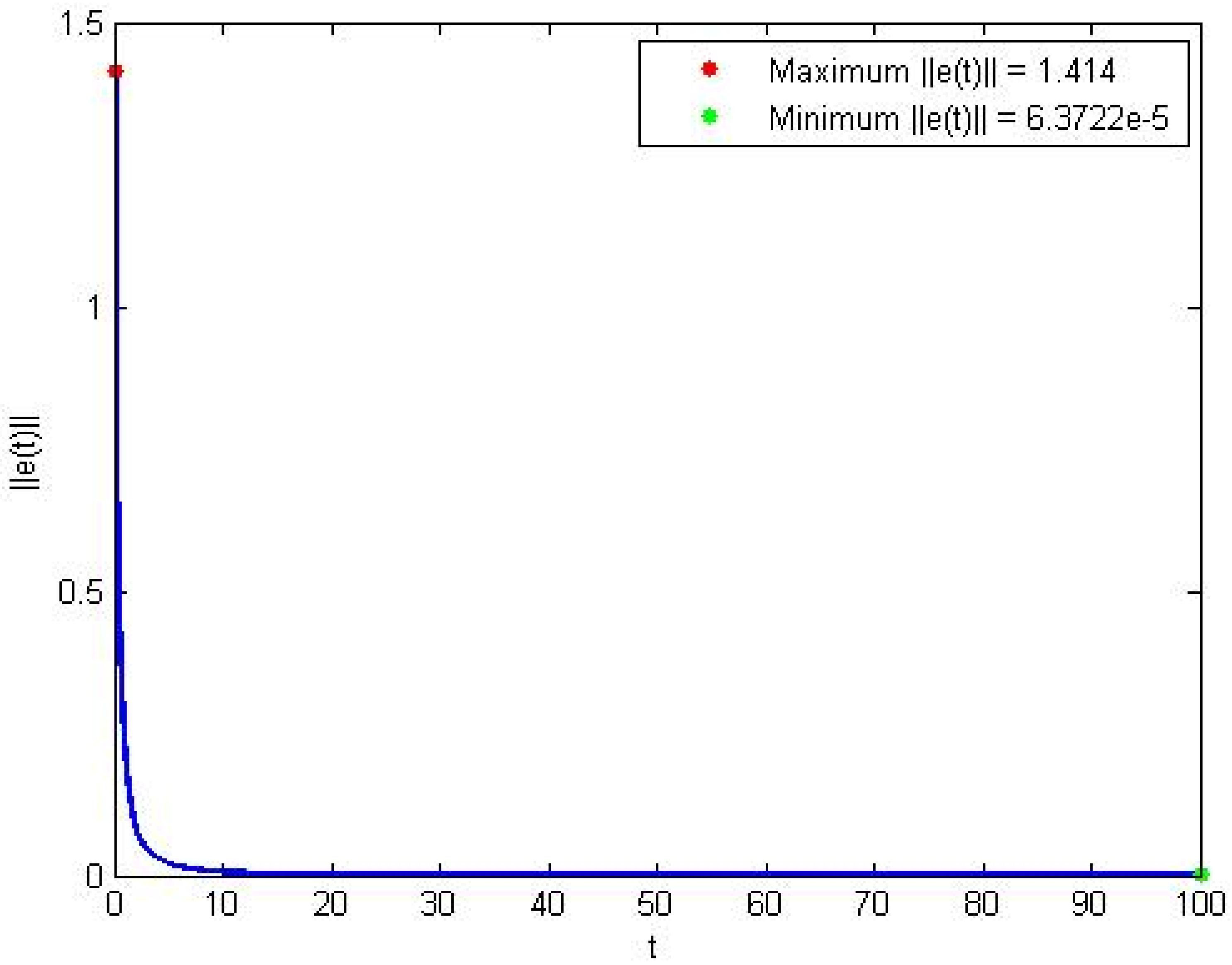
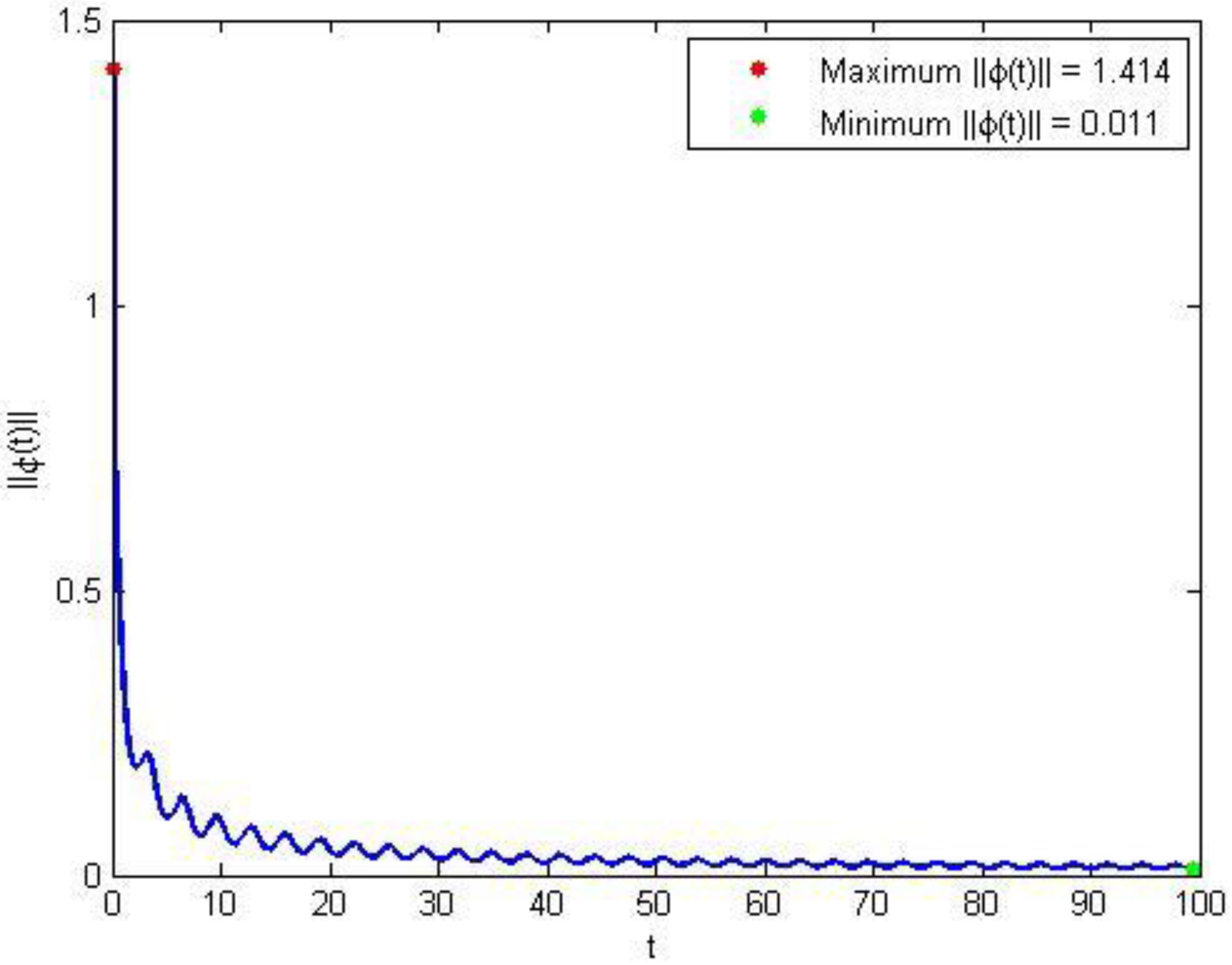
4.1.2. Simulation Study
4.2. Identification Using Fractional Error Model 1 with Parameter Constraints
4.2.1. Theoretical Study
- : In this case, (21)–(23) reduce to the convergence in mean value of , , and , respectively.
- : This case corresponds to the classical Caputo derivative concept. An analogue study has been conducted for Caputo fractional systems in [35].
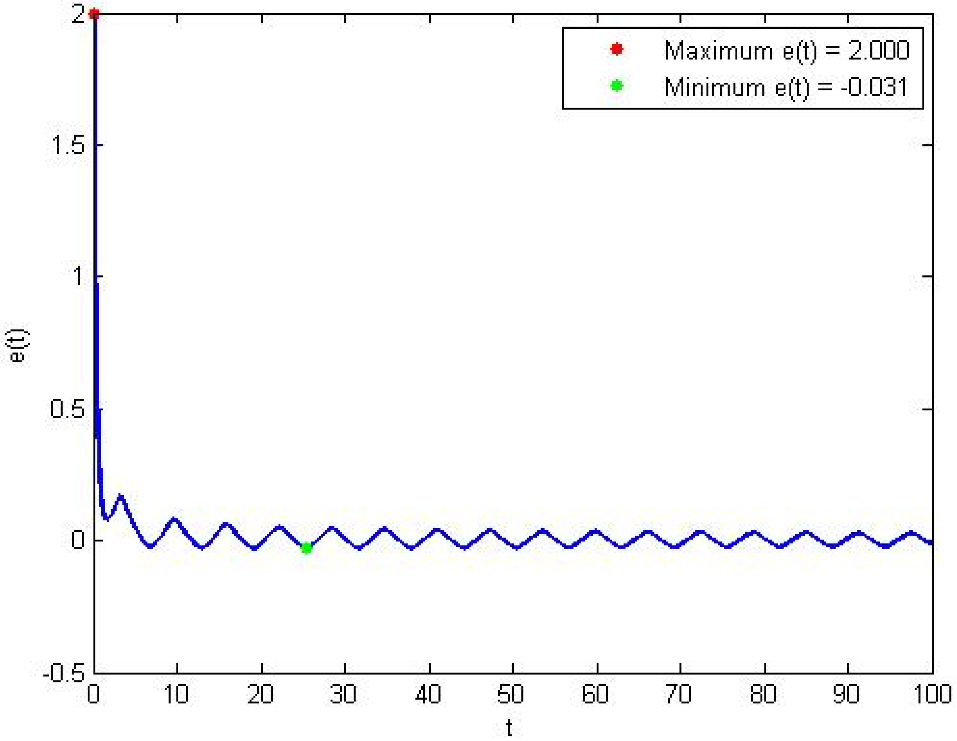
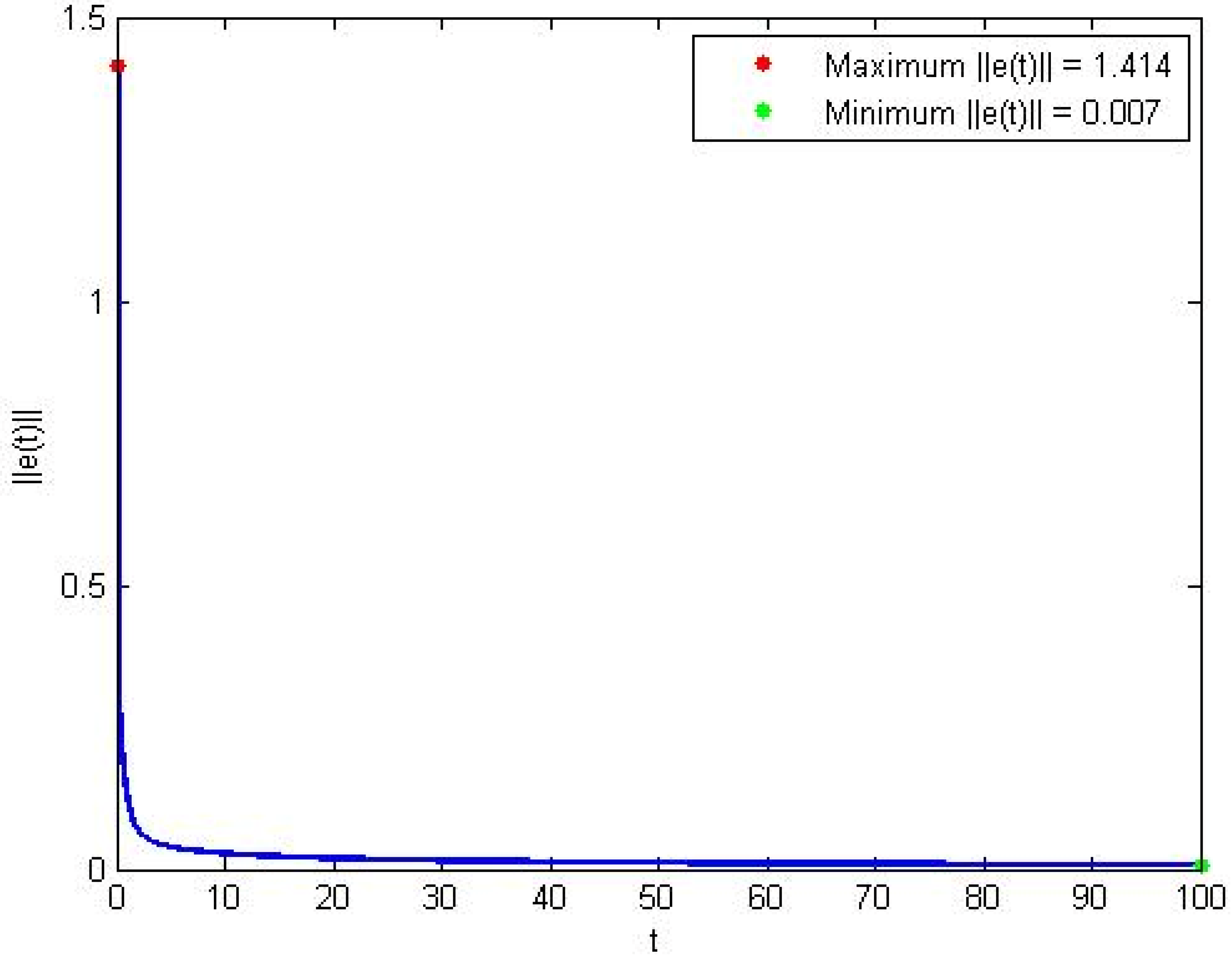
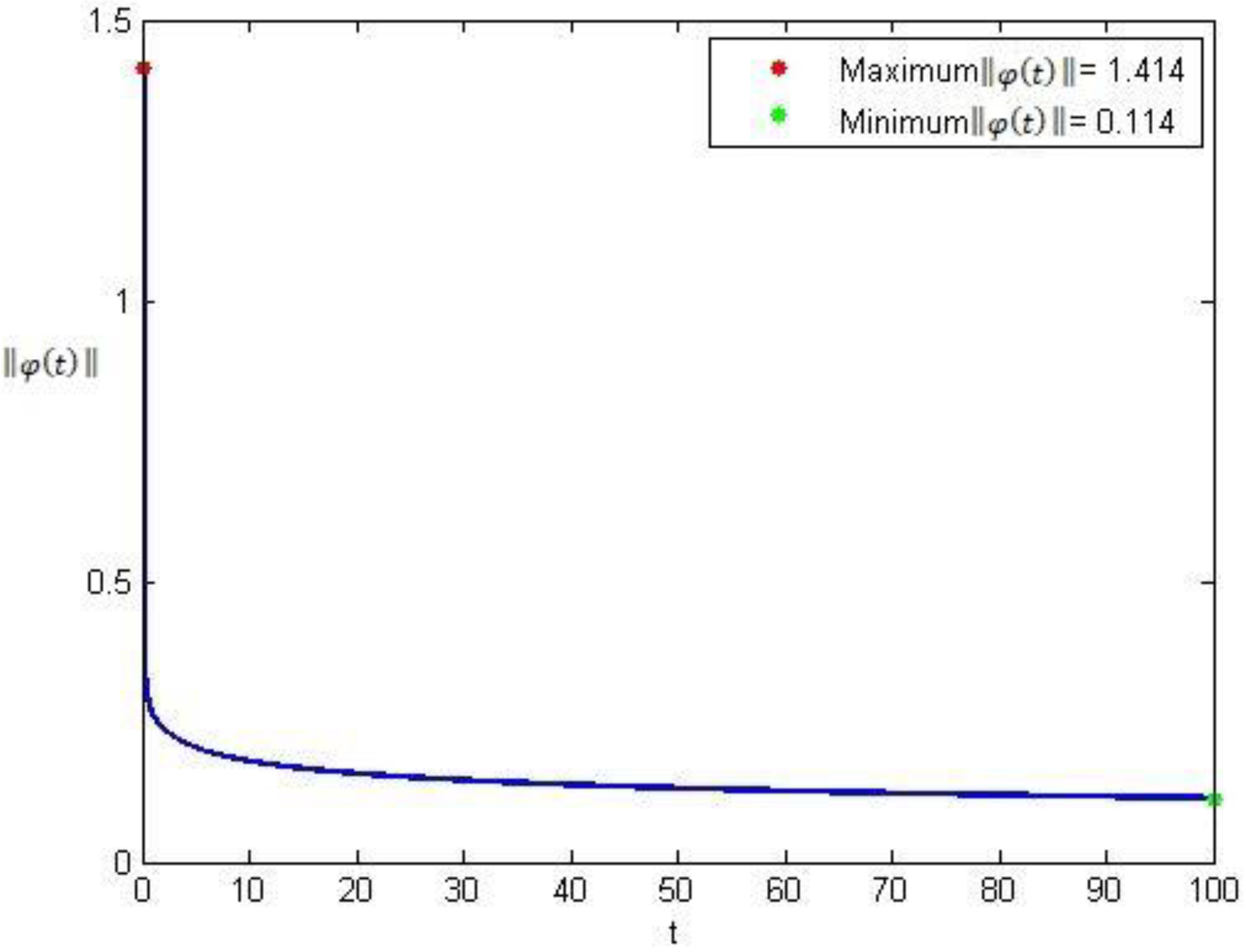
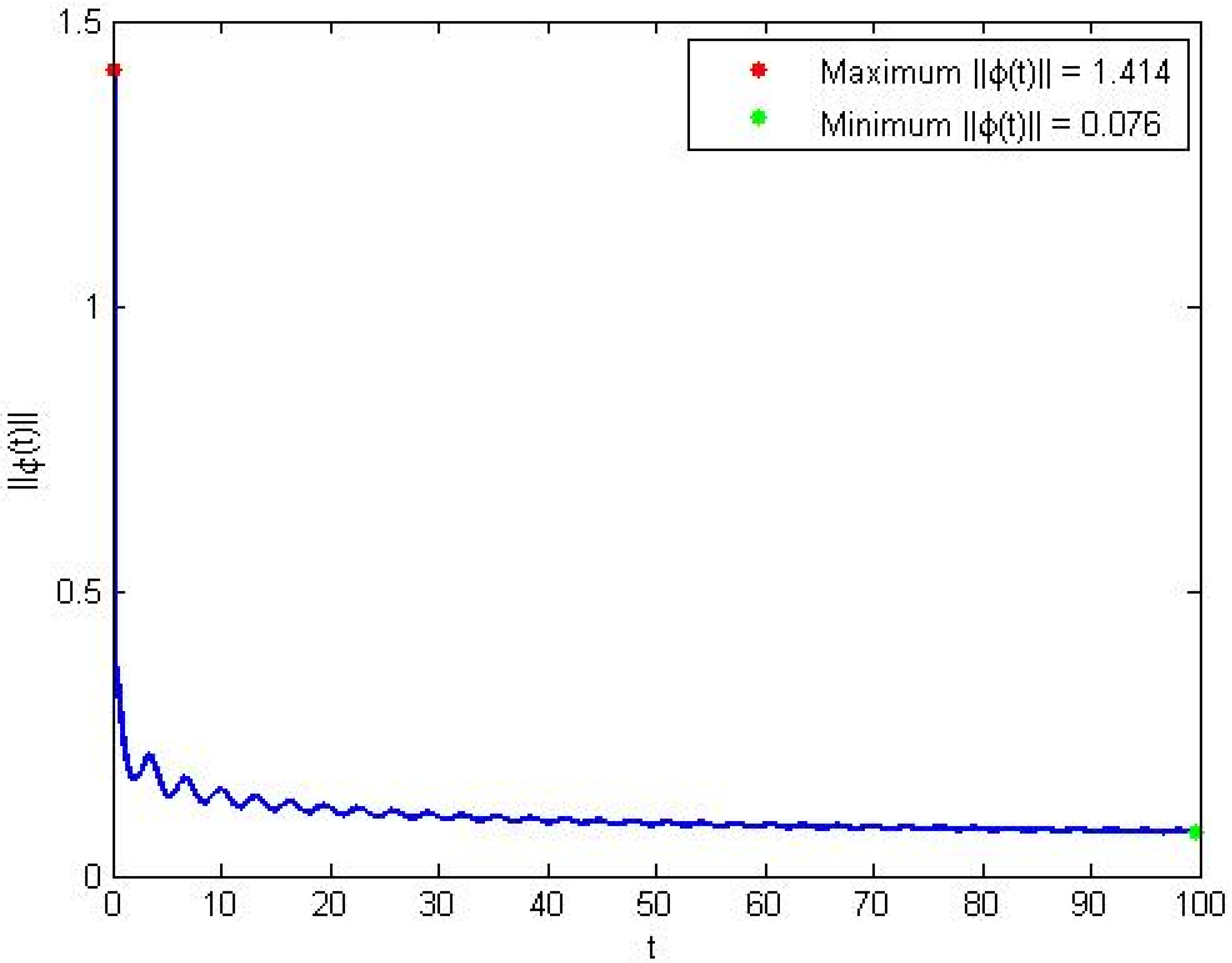
4.2.2. Simulation Study
5. Conclusions
Author Contributions
Funding
Institutional Review Board Statement
Informed Consent Statement
Data Availability Statement
Conflicts of Interest
References
- Engheta, N. On fractional calculus and fractional multipoles in electromagnetism. IEEE Trans. Antennas Propag. 1996, 44, 554–566. [Google Scholar] [CrossRef]
- Laskin, N. Fractional market dynamics. Phys. A Stat. Mech. Its Appl. 2000, 287, 482–492. [Google Scholar] [CrossRef]
- Boutiara, A.; Etemad, S.; Alzabut, J.; Hussain, A.; Subramanian, M.; Rezapour, S. On a nonlinear sequential four-point fractional q-difference equation involving q-integral operators in boundary conditions along with stability criteria. Adv. Differ. Equ. 2021, 2021, 367. [Google Scholar] [CrossRef]
- Boutiara, A.; Benbachir, M. Existence and uniqueness results to a fractional q-difference coupled system with integral boundary conditions via topological degree theory. Int. J. Nonlinear Anal. Appl. 2022, 13, 3197–3211. [Google Scholar]
- Boutiara, A.; Abdo, M.S.; Alqudah, M.A.; Abdeljawad, T. On a class of Langevin equations in the frame of Caputo function-dependent-kernel fractional derivatives with antiperiodic boundary conditions. AIMS Math. 2021, 6, 5518–5534. [Google Scholar] [CrossRef]
- Jmal, A.; Naifar, O.; Ben Makhlouf, A.; Derbel, N.; Hammami, M.A. Robust sensor fault estimation for fractional-order systems with monotone nonlinearities. Nonlinear Dyn. 2017, 90, 2673–2685. [Google Scholar] [CrossRef]
- Adjimi, N.; Boutiara, A.; Abdo, M.S.; Benbachir, M. Existence results for nonlinear neutral generalized Caputo fractional differential equations. J. Pseudo-Differential Oper. Appl. 2021, 12, 1–17. [Google Scholar] [CrossRef]
- Suwan, I.; Abdo, M.; Abdeljawad, T.; Mater, M.; Boutiara, A.; Almalahi, M. Existence theorems for ψ-fractional hybrid systems with periodic boundary conditions. AIMS Math. 2021, 7, 171–186. [Google Scholar] [CrossRef]
- Jmal, A.; Naifar, O.; Ben Makhlouf, A.; Derbel, N.; Hammami, M.A. Observer-based model reference control for linear fractional-order systems. Int. J. Digit. Signals Smart Syst. 2018, 2, 136–149. [Google Scholar] [CrossRef]
- Katugampola, U.N. New approach to a generalized fractional integral. Appl. Math. Comput. 2011, 218, 860–865. [Google Scholar] [CrossRef] [Green Version]
- Katugampola, U.N. A new approach to generalized fractional derivatives. Bull. Math. Anal. Appl. 2014, 6, 1–15. [Google Scholar]
- Katugampola, U.N. Existence and uniqueness results for a class of generalized fractional differential equations. arXiv 2014, arXiv:1411.5229. [Google Scholar]
- Kilbas, A.A.; Srivastava, H.H.; Trujillo, J.J. Theory and Applications of Fractional Differential Equations; Elsevier: Amsterdam, The Netherlands, 2006. [Google Scholar]
- Podlubny, I. Fractional Differential Equations; Academic Press: San Diego, CA, USA, 1999. [Google Scholar]
- Almeida, R. Variational Problems Involving a Caputo-Type Fractional Derivative. J. Optim. Theory Appl. 2016, 174, 276–294. [Google Scholar] [CrossRef]
- Sene, N.; Gómez-Aguilar, J.F. Analytical solutions of electrical circuits considering certain generalized fractional derivatives. Eur. Phys. J. Plus 2019, 134, 260. [Google Scholar] [CrossRef]
- Karkhane, M.; Pourgholi, M. Adaptive observer design for one sided Lipschitz class of nonlinear systems. Modares J. Electr. Eng. 2015, 11, 45–51. [Google Scholar]
- Naifar, O.; Boukettaya, G.; Ouali, A. Global stabilization of an adaptive observer-based controller design applied to induction machine. Int. J. Adv. Manuf. Technol. 2015, 81, 423–432. [Google Scholar] [CrossRef]
- Tao, G. A simple alternative to the Barbalat lemma. IEEE Trans. Autom. Control 1997, 42, 698. [Google Scholar] [CrossRef]
- Aguila-Camacho, N.; Duarte-Mermoud, M.A. Boundedness of the solutions for certain classes of fractional differential equations with application to adaptive systems. ISA Trans. 2016, 60, 82–88. [Google Scholar] [CrossRef]
- Souahi, A.; Naifar, O.; Ben Makhlouf, A.; Hammami, M.A. Discussion on Barbalat Lemma extensions for conformable fractional integrals. Int. J. Control 2017, 92, 234–241. [Google Scholar] [CrossRef]
- Liu, D.Y.; Laleg-Kirati, T.M.; Gibaru, O.; Perruquetti, W. Identification of fractional order systems using modulating functions method. In Proceedings of the American Control Conference (ACC), Washington, DC, USA, 17–19 June 2013; IEEE: Piscataway, NJ, USA, 2013; pp. 1679–1684. [Google Scholar]
- Yuan, L.-G.; Yang, Q.-G. Parameter identification and synchronization of fractional-order chaotic systems. Commun. Nonlinear Sci. Numer. Simul. 2012, 17, 305–316. [Google Scholar] [CrossRef]
- Narendra, K.S.; Annaswamy, A.M. Stable Adaptive Systems; Dover Publications Inc.: Mineola, NY, USA, 2005. [Google Scholar]
- Duarte-Mermoud, A.M.; Aguila-Camacho, N. Some Useful Results in Fractional Adaptive Control. In Proceedings of the Sixteenth Yale Workshop on Adaptive and Learning Systems, New Haven, CT, USA, 5–7 June 2013; pp. 51–56. [Google Scholar]
- Almeida, R.; Malinowska, A.B.; Odzijewicz, T. Fractional Differential Equations with Dependence on the Caputo–Katugampola Derivative. J. Comput. Nonlinear Dyn. 2016, 11, 061017. [Google Scholar] [CrossRef] [Green Version]
- Baleanu, D.; Wu, G.-C.; Zeng, S. Chaos analysis and asymptotic stability of generalized Caputo fractional differential equations. Chaos Solitons Fractals 2017, 102, 99–105. [Google Scholar] [CrossRef]
- Aguila-Camacho, N.; Duarte-Mermoud, M.A. Fractional error model 1 in adaptive systems. In Proceedings of the IEEE International Conference on Fractional Differentiation and Its Applications (ICFDA), Catania, Italy, 23–25 June 2014; pp. 1–5. [Google Scholar]
- Aguila-Camacho, N.; Duarte-Mermoud, M.A. Improved adaptive laws for fractional error models 1 with parameter constraints. Int. J. Dyn. Control 2016, 5, 198–207. [Google Scholar] [CrossRef]
- Duarte-Mermoud, M.A.; Narendra, K.S. Error models with parameter constraints. Int. J. Control 1996, 64, 1089–1111. [Google Scholar] [CrossRef]
- Liu, H.; Pan, Y.; Cao, J.; Wang, H.; Zhou, Y. Adaptive neural network backstepping control of fractional-order nonlinear systems with actuator faults. IEEE Trans. Neural Netw. Learn. Syst. 2020, 31, 5166–5177. [Google Scholar] [CrossRef]
- Chen, J.; Tepljakov, A.; Petlenkov, E.; Chen, Y.; Zhuang, B. Boundary Mittag-Leffler stabilization of coupled time fractional order reaction–advection–diffusion systems with non-constant coefficients. Syst. Control Lett. 2021, 149, 104875. [Google Scholar] [CrossRef]
- Coca, D.; Billings, S.A. Direct parameter identification of distributed parameter systems. Int. J. Syst. Sci. 2000, 31, 11–17. [Google Scholar] [CrossRef]
- Yu, W.; Chen, G.; Cao, J.; Lü, J.; Parlitz, U. Parameter identification of dynamical systems from time series. Phys. Rev. E 2007, 75, 067201. [Google Scholar] [CrossRef]
- Pillai, D.S.; Rajasekar, N. Metaheuristic algorithms for PV parameter identification: A comprehensive review with an application to threshold setting for fault detection in PV systems. Renew. Sustain. Energy Rev. 2018, 82, 3503–3525. [Google Scholar] [CrossRef]


Publisher’s Note: MDPI stays neutral with regard to jurisdictional claims in published maps and institutional affiliations. |
© 2022 by the authors. Licensee MDPI, Basel, Switzerland. This article is an open access article distributed under the terms and conditions of the Creative Commons Attribution (CC BY) license (https://creativecommons.org/licenses/by/4.0/).
Share and Cite
Kahouli, O.; Jmal, A.; Naifar, O.; Nagy, A.M.; Ben Makhlouf, A. New Result for the Analysis of Katugampola Fractional-Order Systems—Application to Identification Problems. Mathematics 2022, 10, 1814. https://doi.org/10.3390/math10111814
Kahouli O, Jmal A, Naifar O, Nagy AM, Ben Makhlouf A. New Result for the Analysis of Katugampola Fractional-Order Systems—Application to Identification Problems. Mathematics. 2022; 10(11):1814. https://doi.org/10.3390/math10111814
Chicago/Turabian StyleKahouli, Omar, Assaad Jmal, Omar Naifar, Abdelhameed M. Nagy, and Abdellatif Ben Makhlouf. 2022. "New Result for the Analysis of Katugampola Fractional-Order Systems—Application to Identification Problems" Mathematics 10, no. 11: 1814. https://doi.org/10.3390/math10111814