Article

Estimation of the Generalized Logarithmic Transformation Exponential Distribution under Progressively Type-II Censored Data with Application to the COVID-19 Mortality Rates

1
Department of Statistics, Faculty of Science, University of Tabuk, Tabuk 47512, Saudi Arabia
2
Department of Mathematics and Statistics, Banasthali Vidyapith, Vanasthali 304022, Rajasthan, India
*
Author to whom correspondence should be addressed.
Mathematics 2022, 10(7), 1015; https://doi.org/10.3390/math10071015
Submission received: 27 January 2022 / Revised: 14 March 2022 / Accepted: 17 March 2022 / Published: 22 March 2022

Abstract

:
In this paper, classical and Bayesian estimation for the parameters and the reliability function for the generalized logarithmic transformation exponential (GLTE) distribution has been proposed when the life-times are progressively censored. The maximum likelihood estimator of unknown parameters and their corresponding reliability function are obtained under the classical setup. The Bayes estimators are obtained for symmetric (squared error) and asymmetric (LINEX and general entropy) loss functions. This was achieved by considering discrete prior for the scale parameter and conditional gamma prior for the shape parameter. Interval estimation of the unknown parameters and reliability function for classical and Bayesian schemes is also considered. The performances of various derived estimators are recorded using simulation study for different sample sizes and progressive censoring schemes. Finally, the COVID-19 mortality data sets are provided to illustrate the computation of various estimators.

1. Introduction

In statistical theory, there are several lifetime probability models which are used to analyse the uncertainty of the random phenomena in various fields, for example, engineering, medical sciences, financial affairs, etc. The most commonly used lifetime model is exponential distribution. This distribution has a simple mathematical form and constant hazard rate which makes this distribution quite useful in real life testing and reliability problems. However, having constant hazard rate sometimes become a hurdle for analysing some situations. To tackle this issue, different probability models were discussed such as Weibull, gamma, Burr, Lindley distribution, etc. Nowadays, we are seeing problems which are complex in nature and the statistical behaviour of such problem change rapidly. So, in such situations, we must have a general form of distributions which can also transform according to our need. In this direction, various generalized family of distributions are proposed by academicians (see [1,2,3,4,5]). Ref. [6] proposed a logarithm transformation (LT) method for obtaining the new family of distributions. The family of distributions proposed by [6] has the following cumulative distribution function (cdf):
F ( x ) = 1 ln ( 2 G ( x ) ) ln 2 , x > 0 .
Proceeding in the same manner, Ref. [7] generalized the results of [6] by introducing a shape parameter in the baseline cdf of Equation (1). The family of distributions proposed by [7] has the following cdf:
F ( x ) = 1 ln ( 2 G α ( x ) ) ln 2 , x > 0 , α > 0 .
To study the properties of (2), the authors considered G ( x ) = 1 e θ x , x > 0 , θ > 0 (exponential baseline distribution) and called it generalized logarithm transformation exponential (GLTE) distribution. The pdf and cdf of GLTE distribution are given as
f ( x ) = α θ e θ x 1 e θ x α 1 ( 2 ( 1 e θ x ) α ) ln 2 , x > 0 , θ , α > 0 0 , otherwise .
F ( x ) = 1 ln ( 2 ( 1 e θ x ) α ) ln 2 , x > 0 , θ , α > 0 .
respectively. The reliability function and hazard rate function of GLTE distribution are given as
R ( t ) = 1 F ( t ) = ln ( 2 ( 1 e θ t ) α ) ln 2 , t > 0 , θ , α > 0 .
and
H ( t ) = f ( t ) R ( t ) = α θ e θ x 1 e θ x α 1 ( 2 ( 1 e θ x ) α ) ln ( 2 ( 1 e θ t ) α ) , t > 0 , θ , α > 0 .
The authors of [7] have extensively discussed the behaviour of hazard rate function for different values of the parameters. The authors observed that for α 1 GLTE distribution is depicting increasing hazard rate, for α 0.5 , GLTE distribution is depicting decreasing hazard rate. The authors also emphasized that the distribution has a bathtub hazard rate. These results are depicted in Figure 2 of [7].
Ref. [7] considered classical and Bayesian estimation of GLTE distributions of unknown parameters under type-II censoring scheme. To the best of our knowledge, until now no attempt has been made to estimate the parameters and reliability characteristic for GLTE distribution other than the type-II censoring scheme. This is why we have considered progressive type-II censoring scheme for our study which is a generalize form of type-II censoring scheme. Hence, the results of this paper are of more general in nature. In addition to that the GLTE distribution provides a better fit to the considered demographic data (mortality rates) over other lifetime distributions e.g., Weibull, Chen, etc. (see Section 5). Keeping these points in mind, we have discussed the classical as well as the Bayesian estimation and reliability characteristics for the GLTE distribution under the progressive type-II censored data.
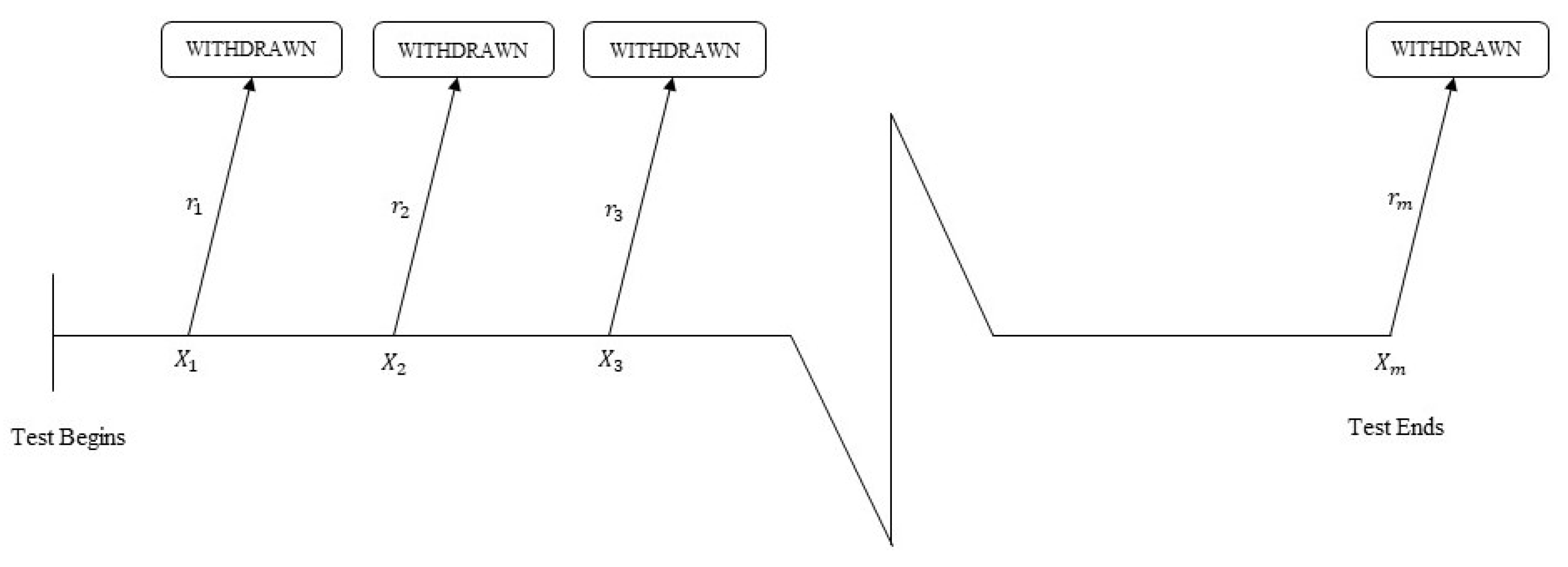
In any life-testing experiment, it is very cumbersome to complete the experiment for a long time period due to time and cost constraints. There are various types of censoring schemes which have been introduced in the literature to reduce the time and cost involved into the experiments. Type-I and Type-II are the most common censoring schemes among the various censoring schemes. The number of observed failures in the type-I censoring scheme is random in nature, whereas the termination time of the experiments is random in the type-II censoring scheme. Surviving units cannot be withdrawn during the experimentation of these two schemes. The main advantage of progressive censoring is that it saves a lot of energy and money due to its ability to drop live units from the experiment in practical failure time experiment. Initially, the progressive censoring scheme was proposed by [8].
Let n units are put on test at the same time. If first failure occurs at the time X 1 , r 1 surviving units are randomly removed from the experiment. At the second failure time X 2 , r 2 surviving units are randomly removed from the remaining surviving units. The experiment continues until the m th failure time X m observed. At this time, the test can be terminated with removing all the surviving units from the experiment. Here, X = ( X 1 , X 2 , . . . , X m ) is a set of observed life-time, referred to as progressively type-II censored sample (see, Figure 1). In the case of r 1 = r 2 = . . . = r m 1 = 0 , this scheme becomes type-II censoring scheme. It is also observed that for r 1 = r 2 = . . . = r m = 0 , this scheme transformed into the case of complete sample.
In the last few years, progressive censoring scheme has received considerable attention (see [9,10,11]). Ref. [12] has made a remarkable contribution to developments, implementations and other dimensions of progressive censoring. The progressive censored data for the Burr model was discussed by [13]. The Bayesian inference for the Weibull distribution under progressive censoring scheme was discussed by [14]. The progressive type-II censoring scheme was discussed by [15] for exponential Weibull model and for the inverted exponential model was discussed by [16]. The scheme of progressive censoring for the Burr type-XII and Inverse Weibull were proposed by [17,18], respectively. Ref. [19] have developed a method of estimation for xgamma distribution under progressive type-II censoring approach. Ref. [20] have discussed progressive censoring scheme for lognormal distribution and [21] have discussed Bayesian inference of Hjorth distribution under the progressive type-II censoring scheme. Recently, Ref. [22] addressed the problem of Bayesian reliability estimation for the Topp–Leone distribution based on progressive type-II censoring scheme. The authors obtained Bayes estimators using approximation techniques such as Lindley’s approximation, MCMC and Tierney-Kadane method ([23]).
In this paper, we address the problem of classical and Bayesian estimation of GLTE distribution under the progressive type-II censored data. For the scale parameter, a discrete prior is considered, whereas a conditional gamma prior for the shape parameter is considered. The rest of the paper, we organized as follows: In Section 2, the Maximum likelihood estimators and asymptotic confidence intervals are obtained for the parameters and the reliability function of GLTE distribution. The Bayes estimators under symmetric, asymmetric loss functions and highest posterior density intervals are obtained in Section 3. In Section 4, a simulation study is presented to report the performances of the point and interval estimators. In Section 5, the mortality data sets of Italy and The Netherlands due to COVID-19 are provided to illustrate the computation of various derived results. Finally, the conclusions appear in Section 6.

2. Maximum Likelihood Estimation and Asymptotic Confidence Interval

Suppose X = ( X 1 , X 2 , . . . , X m ) is a progressive type-II censored sample from a life test on n units having the GLTE ( θ , α ) distribution with density given in (1) and r 1 , r 2 , . . . , r m denote the corresponding number of units removed from the test. The likelihood function based on the progressively type-II censored sample is given by
l ( θ , α | x ) = A i = 1 m f ( x i ; θ , α ) 1 F ( x i ; θ , α ) r i ,
where, x = ( x 1 , x 2 , . . . , x m ) and A = n ( n 1 r 1 ) ( n 2 r 1 r 2 ) . . . ( n i = 1 m 1 ( r i + 1 ) ) ; and f ( x ) and F ( x ) are given respectively by (1) and (2).
Substituting (1) and (2), into (7), the likelihood function is
l ( θ , α | x ) = A i = 1 m α θ e θ x i ( 1 e θ x i ) α 1 ( 2 ( 1 e θ x i ) α ) ln 2 ln ( 2 ( 1 e θ x i ) α ) ln 2 r i .
The log-likelihood function can be written as
L = ln l ( θ , α | x ) = ln A + m ln α θ ln 2 + ( α 1 ) i = 1 m ln ( 1 e θ x i ) θ i = 1 m x i i = 1 m ln ( 2 ( 1 e θ x i ) α ) + i = 1 m r i ln ( 2 ( 1 e θ x i ) α ) ln 2 ,
L α = m α + i = 1 m ln ( 1 e θ x i ) + i = 1 m ( 1 e θ x i ) α ln ( 1 e θ x i ) ( 2 ( 1 e θ x i ) α ) + i = 1 m r i ( 1 e θ x i ) α ln ( 1 e θ x i ) ( 2 ( 1 e θ x i ) α ) ln 2 = 0 ,
and
L θ = m θ i = 1 m x i + ( α 1 ) i = 1 m x i e θ x i 1 e θ x i + α x i ( 1 e θ x i ) α 1 ( 1 e θ x i ) ( 2 ( 1 e θ x i ) α ) + i = 1 m r i α x i ( 1 e θ x i ) α 1 ( 1 e θ x i ) ( 2 ( 1 e θ x i ) α ) ln 2 = 0 .
It is clear that the Equations (10) and (11) are of implicit forms and are non-linear in nature, so, MLEs of unknown parameters are tedious to obtain, analytically. Thus, one may use any numerical approximation techniques, such as Newton–Raphson (N-R) method, fixed-point iterations, etc. Here, we used the N-R method to evaluate the MLE of the parameters with the help of R Software. Once the MLEs of the parameters are obtained from Equations (10) and (11), the MLE of reliability function is evaluated using the invariance property and is given in (12)
R ( t ) = ln ( 2 ( 1 e θ ^ t ) α ^ ) ln 2 .
Further, using the property MLE, we obtained the asymptotic confidence intervals (ACIs) for α , θ and R ( t ) . The ACIs are obtained from the diagonal elements of the inverse Fisher information matrix that gives the asymptotic variance for the parameters α and θ respectively. Thus, the 100 1 η % confidence interval for α , θ and R ( t ) can be defined respectively, as α ^ Z η / 2 v a r ( α ^ ) , α ^ + Z η / 2 v a r ( α ^ ) ,   θ ^ Z η / 2 v a r ( θ ^ ) , θ ^ + Z η / 2 v a r ( θ ^ ) ,   R ( t ) ^ Z η / 2 v a r R ( t ) ^ , R ( t ) ^ + Z η / 2 v a r R ( t ) ^ , where Z η / 2 is a standard normal variate.

3. Bayesian Estimation

In this section, we consider both parameters shape as well as scale as unknown for GLTE distribution. To estimate these parameters, we adopt the method proposed by [24]. Several researchers also used this method (see, [25,26]). Here, the scale parameter θ is restricted to a finite number of values θ 1 , θ 2 , . . . , θ N with probabilities η 1 , η 2 , . . . , η N respectively, the prior distribution for θ is given by
j = 1 N η j = 1 , 0 η j 1 , P r ( θ = θ j ) = η j , j = 1 , 2 , . . . , N .
Further, we consider conditional gamma prior for parameter α over θ = θ j with hyper parameters a j and b j ,
π ( α | θ j , x ) = b j a j α a j 1 e b j α Γ ( a j ) , α > 0 , a j , b j > 0 .
Here, we consider symmetric (squared error) and asymmetric (LINEX and general entropy) loss functions to obtain the Bayes estimators of unknown parameters and reliability function of the distribution. The likelihood function (8) in terms of continuous parameter α and discrete parameter θ j is
l ( θ j , α | x ) = A i = 1 m α θ j e θ j x i ( 1 e θ j x i ) α 1 ( 2 ( 1 e θ j x i ) α ) ln 2 ln ( 2 ( 1 e θ j x i ) α ) ln 2 r i .
The joint posterior of α and θ = θ j is
π ( α , θ j | x ) = π ( α | θ j ) P r ( θ = θ j ) l ( θ j , α | x ) 0 j = 1 N π ( α | θ j ) P r ( θ = θ j ) l ( θ j , α | x ) d α = T 1 T 0
where,
T 1 = i = 1 m α θ j e θ j x i ( 1 e θ j x i ) α 1 ( 2 ( 1 e θ j x i ) α ) ln 2 ln ( 2 ( 1 e θ j x i ) α ) ln 2 r i b j a j α a j 1 e b j α Γ ( a j ) η j ,
and
T 0 = 0 j = 1 N T 1 d α .
The marginal posterior density of θ j is obtained by integrating (15) with respect to α , we get
P j = 0 π ( α , θ j | x ) d α .
Combining the likelihood function (14) and prior density (13), we obtain the posterior density of α
π ( α | θ j , x ) = π ( α | θ j ) l ( θ j , α | x ) 0 π ( α | θ j ) l ( θ j , α | x ) d α = K 1 K 0
where,
K 1 = i = 1 m α θ j e θ j x i ( 1 e θ j x i ) α 1 ( 2 ( 1 e θ j x i ) α ) ln 2 ln ( 2 ( 1 e θ j x i ) α ) ln 2 r i b j a j α a j 1 e b j α Γ ( a j ) ,
and
K 0 = 0 K 1 d α .

3.1. Bayes Estimation under Symmetric Loss Function

Squared Error Loss Function (SELF): In the SELF, the magnitude of underestimation and overestimation are equal. It is also known as Quadratic loss function. In the SELF, Bayes estimator is represented by the posterior mean. The squared error loss function is defined as
L ( δ ^ , δ ) = ( δ ^ δ ) 2 , δ ^ D , δ Θ ,
where, δ ^ is the Bayes estimator of δ . D is a decision space and Θ is parameter space.
The Bayes estimators α ˜ B S and θ ˜ B S of parameters α and θ , respectively, are
α ˜ B S = 0 j = 1 N P j α π ( α | θ j , x ) d α = 0 j = 1 N P j α K 1 K 0 d α α ˜ B S = 1 K 0 0 α j = 1 N P j K 1 d α . θ ˜ B S = j = 1 N θ j P j .
The Bayes estimator R ˜ B S ( t ) of the reliability function R ( t ) is
R ˜ B S ( t ) = 0 j = 1 N P j ln ( 2 ( 1 e θ j t ) α ) ln 2 π ( α | θ j , x ) d α = 0 j = 1 N P j ln ( 2 ( 1 e θ j t ) α ) ln 2 K 1 K 0 d α = 1 K 0 0 j = 1 N P j K 1 ln ( 2 ( 1 e θ j t ) α ) ln 2 d α .

3.2. Bayes Estimation under Asymmetric Loss Function

When the magnitude of overestimation and underestimation are not equal, then we used the asymmetric loss function. In the asymmetric loss function, we consider LINEX loss function and General Entropy loss function.
LINEX Loss function: The LINEX loss function is defined as
L ( δ ^ δ ) e c ( δ ^ δ ) c ( δ ^ δ ) 1 , c 0 , δ ^ D , δ Θ .
The Bayes estimator δ ^ B L of δ under the LINEX loss function is
δ ^ B L = 1 c ln [ E δ ( e x p ( c δ ) ) ] ,
provided, E δ ( e x p ( c δ ) ) exists and finite. The Bayes estimators α ˜ B L and θ ˜ B L of parameters α and θ under LINEX loss function (18), respectively, are
α ˜ B L = 1 c ln 0 j = 1 N P j e x p ( c α ) K 1 K 0 d α α ˜ B L = 1 a K 0 ln 0 j = 1 N P j K 1 e x p ( c α ) d α . θ ˜ B L = 1 c ln j = 1 N P j e x p ( c θ j ) .
The Bayes estimators R ˜ B L ( t ) of the reliability function R ( t ) is
R ˜ B L ( t ) = 1 c ln 0 j = 1 N P j e x p c ln ( 2 ( 1 e θ j t ) α ) ln 2 K 1 K 0 d α = 1 c K 0 ln 0 j = 1 N P j K 1 e x p c ln ( 2 ( 1 e θ j t ) α ) ln 2 d α .
General Entropy Loss Function: The General Entropy loss function is defined as
L ( δ ^ , δ ) δ ^ δ q q ln δ ^ δ 1 , q 0 , δ ^ D , δ Θ .
The Bayes estimator δ ^ B G of δ under GE loss function is
δ ^ B G = E δ ( δ q ) 1 q ,
provided, E δ ( δ q ) exists and is finite.
The Bayes estimators α ˜ B G and θ ˜ B G of parameters α and θ under General Entropy loss function (19), respectively, are
α ˜ B G = 0 j = 1 N P j α q K 1 K 0 d α 1 q α ˜ B G = 1 K 0 0 α q j = 1 N P j K 1 d α 1 q . θ ˜ B G = j = 1 N P j θ j q 1 q .
The Bayes estimator R ˜ B G ( t ) of the reliability function R ( t ) is
R ˜ B G ( t ) = 0 j = 1 N P j ln ( 2 ( 1 e θ j t ) α ) ln 2 q K 1 K 0 d α 1 q = 1 K 0 0 j = 1 N P j K 1 ln ( 2 ( 1 e θ j t ) α ) ln 2 q d α 1 q .

3.3. Bayesian Credible Interval

In the Bayesian paradigm, parameter τ is a random variable and the probability for this parameter τ lies within the specified intervals. The highest posterior density (HPD) interval was discussed by [27]. The HPD interval is the shortest interval among all Bayesian intervals. The HPD interval for parameter τ based on the samples from simulation method ie., τ 1 , τ 2 , , τ M was discussed by [28] (see [29,30]). The algorithm to obtain the HPD interval is as follows
(i) 
In the first step, we generate a random censored data from GLTE distribution using Equation (4) for some fixed values of the parameters using different censoring schemes.
(ii) 
After this, we use the results of MLEs and Bayes estimators derived in Section 2 and Section 3, respectively, to calculate the required estimators (say τ ) with the help of the generated data in step (i).
(iii) 
We repeat the steps (i–ii) N times and obtain the N values of the estimators i.e., τ 1 , τ 2 , , τ N .
(iv) 
Now we apply the method of [28] and obtain the Bayes credible interval.

4. Simulation Study

In this section, we perform a simulation study for the GLTE distribution under the progressive type-II censored sample. This simulation study is conducted to measure the performances of various estimators obtained in this article. The algorithm for generation of progressive type-II censored sample was given by [31]. The algorithm is modified according to our problem and is given as:
  • Generate m iid random numbers W 1 , W 2 , , W m from U ( 0 , 1 ) .
  • Determine the values of the censored scheme r i , for i = 1 , 2 , , m .
  • Set V i = W i 1 / ( i + j = m i + 1 m r j ) for i = 1 , 2 , , m .
  • Set U i = 1 V m V m 1 . . . V m i + 1 , i = 1 , 2 , m . Then { U i , i = 1 , 2 , , m } is the progressive type-II censored sample from U ( 0 , 1 ) .
  • Set
    X i = F 1 ( U i ) = 1 θ ln [ 1 ( 2 2 ( 1 U i ) ) 1 / α ] , i = 1 , 2 , , m .
    Now, X 1 , X 2 , , X m is the progressive type-II censored sample from GLTE distribution.
The performances of estimators are measured by using the criteria of mean square error (MSE) and expected risk (ER). The values of MSEs and ERs are calculated for various configuration of parameters ( α , θ ) i.e., ( 1 , 1.5 ) , ( 1.2 , 1.5 ) . We have also considered few censoring schemes (C.S.) which are defined
*
R 1 = r 1 , r 2 , , r m 1 = 1 , r m = n 2 m + 1 .
*
R 2 = r 1 = n 2 m + 1 , r 2 = r 3 = = r m = 1 .
*
R 3 = r 1 = n m , r 2 = r 3 = r m = 0 .
In order to calculate MSEs and ERs, we replicated our results 1000 times. All the calculated results are reported in Table 1, Table 2, Table 3, Table 4, Table 5, Table 6, Table 7, Table 8, Table 9 and Table 10. The following observations are made from the calculated tables.
(1)
Table 1 and Table 3 show MSEs of the α , θ and R ( t ) for the configuration of ( α , θ ) = ( 1 , 1.5 ) . It can be observed that Bayes estimates of α , θ and R ( t ) show less MSEs in comparison to MLEs. Furthermore, we observe that Bayes estimator under LINEX loss function for c = 0.5 performs better among other Bayes estimators. In terms of R ( t ) , all Bayes estimators perform approximately the same with small MSEs.
(2)
Table 2 and Table 4 show MSEs of the α , θ and R ( t ) for the configuration of ( α , θ ) = ( 1.2 , 1.5 ) . It is observed that Bayes estimates of α , θ and R ( t ) show less MSEs in comparison to MLEs. Moreover, we observe that Bayes estimator under LINEX loss function performs better among other Bayes estimators. In terms of R ( t ) , all estimators perform approximately the same with small MSEs.
(3)
Table 5 and Table 7 report ERs of various Bayes estimators for parameters ( α , θ ) = (1,1.5), respectively. From Tables, we observe that Bayes estimator for LINEX loss function at c = 0.5 exhibits lowest MSEs among other Bayes estimators. In terms of R ( t ) , all estimators perform approximately the same with small MSEs.
(4)
Table 6 and Table 8 report ERs of various Bayes estimators for parameters ( α , θ ) = (1.2,1.5), respectively. We can observe that Bayes estimator for LINEX loss function at c = 0.5 and for GE loss function at q = 0.5 exhibits lower ERs among other Bayes estimates for the parameters α and θ , respectively. In terms of R ( t ) , all estimators perform approximately the same with small MSEs, but Bayes estimators seem to perform slightly better.
(5)
Table 9 and Table 10 show the average length of ACIs and HPD intervals of parameters α , θ and R ( t ) , respectively. It is observed that the average lengths of the intervals decreases when the different choices of n , r increases for both classical and Bayesian estimation. We also observe that HPD intervals of the estimators under LINEX loss function are mostly better among other estimators.
From Table 1, Table 2, Table 3, Table 4, Table 5, Table 6, Table 7, Table 8, Table 9 and Table 10, we conclude that, for different choices of the parameters ( α , θ ) = ( 1 , 1.5 ) , ( 1.2 , 1.5 ) , the Bayes estimator under asymmetric loss function i.e., LINEX loss function shows less MSEs and ERs. Hence, it performs better than other estimators. It is worth mentioning here that for very few cases, the Bayes estimator under GE loss function performs better in terms of ERs. In terms of R ( t ) , we observe that the MLEs and Bayes estimators perform approximately the same. On the other hand, when we consider the performances of reliability estimates in term of ERs, we see that Bayes estimators under asymmetric loss functions exhibit lower values in comparison to symmetric loss function and MLE. The censoring scheme R 3 performs better among all the censoring schemes ( R 1 and R 2 ). All the above observations are made for increasing values of n and m .

5. Real Data

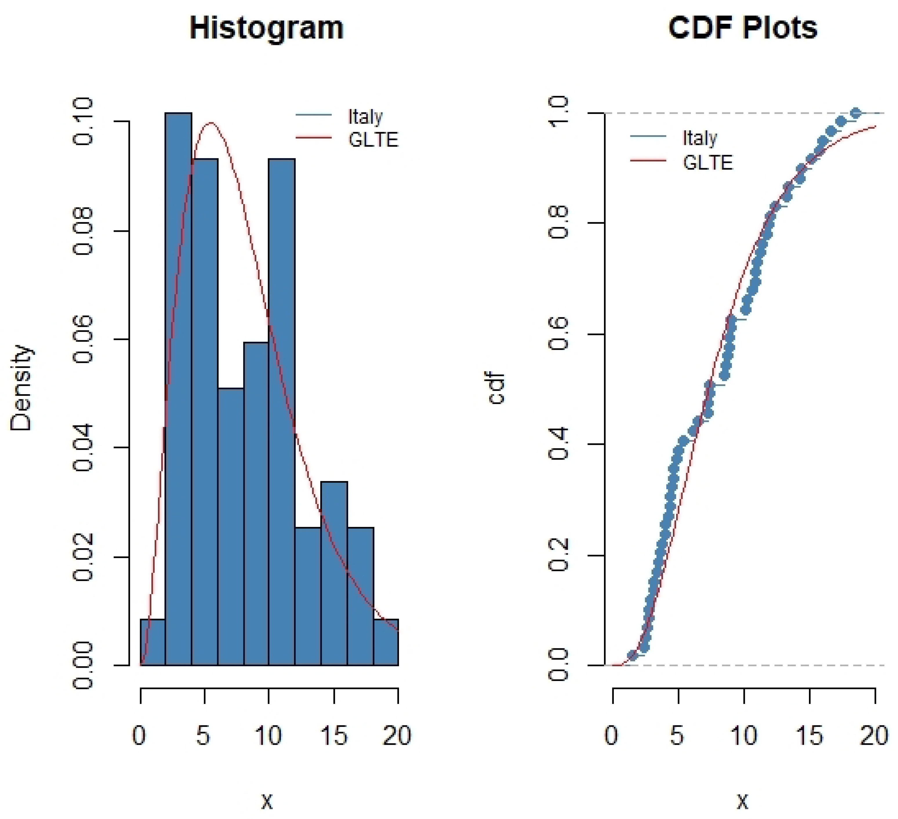
In this section, we consider the mortality data sets of Italy and The Netherlands due to COVID-19. The COVID-19 (coronavirus disease) was declared as a pandemic by World Health Organization (WHO) in 2020. It is the third-highest cause of deaths in 2020, as revealed by the US Centers for Disease Control and Prevention (CDC). The mortality rate was calculated through the ratio of number of deaths and total number of cases (reported cases per 100,000). The mortality rate due to COVID-19 increased by 15.9% from 2019 (see, https://www.pharmaceutical-technology.com/comment/covid-19-cause-death-2020/ (accessed on 26 January 2022)). Here, these two COVID-19 data sets represent the mortality rates for 59 days and 30 days of Italy and The Netherlands, respectively (see, https://covid19.who.int/ (accessed on 26 January 2022)). The mortality rates of Italy recorded from 27 February to 27 April 2020 is given in Table 11. 
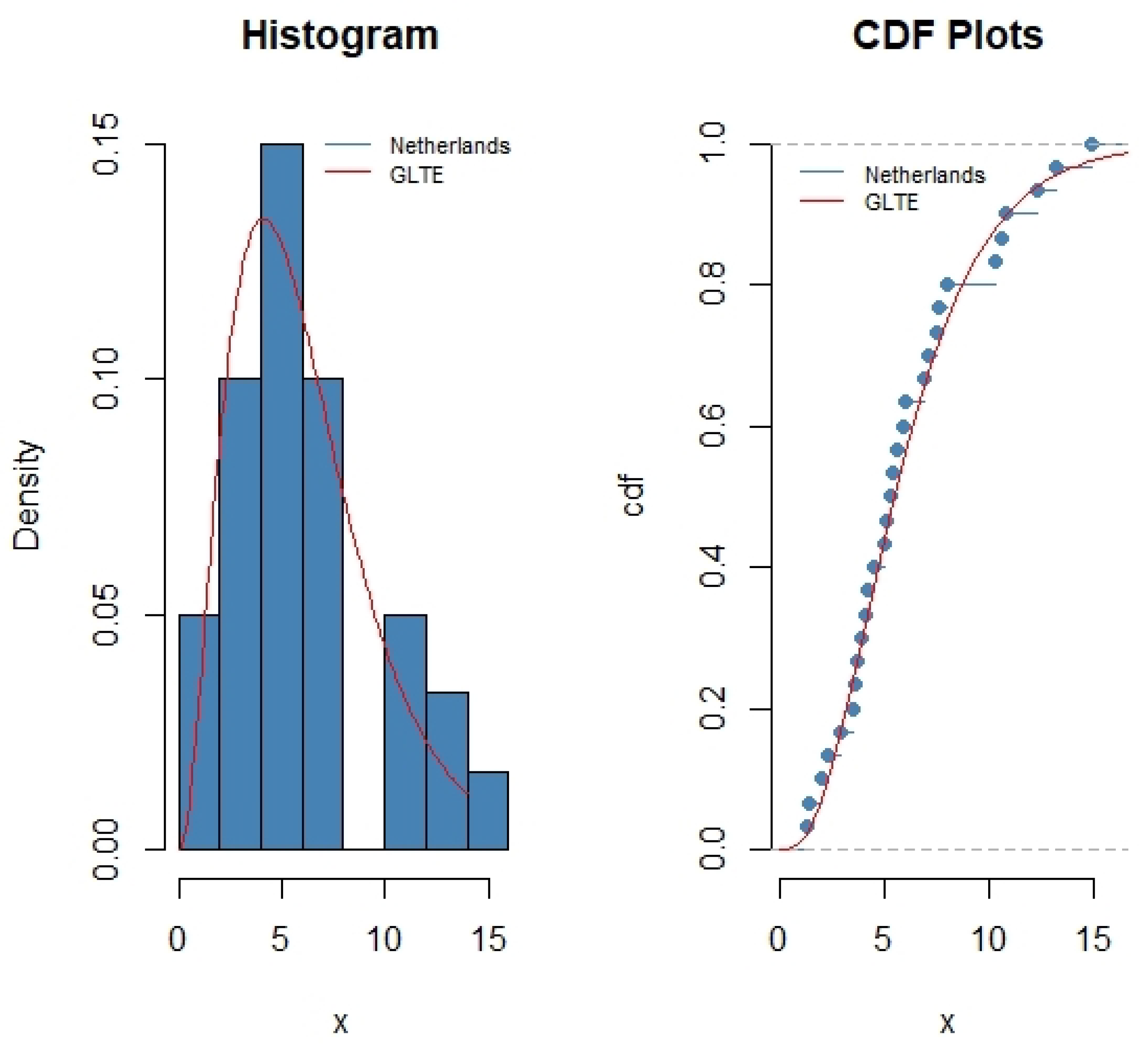
Table 12 represents the mortality rates of The Netherlands recorded from 31 March to 30 April 2020 (also see [32]).
In the terms of suitable fitting of the distribution, the GLTE distribution is compared with other related distributions such as exponential distribution, Weibull distribution, and Chen distribution (see Table 13 and Table 14). The considered real data set was measured on the basis of -Log L which is the negative of the logarithmic value of likelihood, and Kolmogorov–Smirnov (K-S) test statistic for the distribution selection criterion. We also used Akaike Information Criterion (AIC) and Bayesian Information Criterion (BIC). The AIC and BIC are defined as
A I C = 2 × k 2 × l o g L ^ , B I C = k × l o g ( n ) 2 × l o g L ^
where k = Number of parameters, n = Sample size and L ^ = value of the maximum likelihood for the considered distribution. The K-S test statistic D is defined as
D = S u p F n x F x ,
where, F n ( x ) = Empirical distribution function. From Table 13 and Table 14, we observe that the value of AIC, BIC and -Log L of the GLTE distribution is minimum among other distributions. The minimum value of AIC, BIC and -Log L shows that the GLTE distribution better fits for the considered real data sets rather than the other distributions. We observe that Italy’s mortality rates for 59 days supports GLTE distribution with the K-S distance as 0.1137 and p-value as 0.3998 for α = 3.3501 and θ = 0.2626 (see Figure 2). The Netherlands’s mortality rates for 30 days also supports GLTE distribution with the K-S distance as 0.0790 and p-value as 0.9845 for α = 3.4564 and θ = 0.3542 (see Figure 3).
Now, we consider censoring schemes ( R 1 , R 2 , R 3 ) which are used in the simulation study to generate progressive type-II censored samples from the data set of 59 days of mortality rates of Italy of size m = 15 and m = 25 . For the data set of 30 days of mortality rates of The Netherlands of size m = 5 and m = 15 for the same censoring schemes.
For both the data sets of COVID-19, we calculate the Bayes estimators under symmetric and asymmetric loss functions. For asymmetric loss function, we consider c = { 0.5 , 0.5 } in LINEX loss function and q = { 0.5 , 0.5 } in GE loss functions. The calculated Bayes estimates of α , θ and R ( t ) as t = 0.1 are given in Table 15 and Table 16.

6. Conclusions

In this paper, we consider the classical and Bayesian estimation of the unknown parameters and reliability function of the GLTE distribution when the data are progressively type-II censored. The MLEs and Bayes estimators of the parameters and reliability function are obtained. The Bayes estimators were computed using discrete prior for scale parameter and a conditional gamma prior for the shape parameter. We used symmetric (squared error) and asymmetric (LINEX, General Entropy) loss functions to compute the MSEs and ERs. We also address the problem of interval estimation under classical and Bayesian scheme and we derived asymptotic confidence and highest posterior density intervals. The simulation study was done for the different choices of parameter combinations to report the performances of the various estimators, along with the different sample sizes and censoring schemes.
The significance of GLTE distribution over other lifetime distributions such as Weibull, exponential and Chen are discussed in this paper. For this purpose, we considered two real data sets reporting mortality rates of two countries i.e., The Netherlands and Italy. We used the Akaike information and Bayesian information criteria to show the comparison among the probability distributions. The dominance of GLTE distribution over other probability distributions is discussed for the considered data sets of this study. From the simulation study, it is observed that Bayes estimator under LINEX loss function is performing better in most of the cases. It is also worth mentioning that the censoring scheme R 3 works quite well among other schemes considered in this study. So, in real-life situation we should incline our study towards the asymmetric loss function i.e., LINEX and censoring scheme R 3 . All the results and conclusions are based on the problem which is considered in this study.

Author Contributions

O.A. and N.C.K. conceived of the presented idea and O.A. took charge of funding acquisition. N.C.K. and Q.J.A. developed the theory and N.C.K. supervised. Q.J.A. and R.H. performed the computations. R.H. and B.S.O.A. wrote the manuscript with input from all the authors. All authors have read and agreed to the published version of the manuscript.

Funding

This research did not receive external funding.

Institutional Review Board Statement

Not Applicable.

Informed Consent Statement

Not Applicable.

Data Availability Statement

Not Applicable.

Acknowledgments

The authors are thankful to the editor and anonymous referees for their constructive and helpful comments which have significantly improved the article.

Conflicts of Interest

The authors declare no conflict of interest.

References

  1. Mudholkar, G.S.; Srivastava, D.K. Exponentiated Weibull family for analyzing bathtub failure-rate data. IEEE Trans. Reliab. 1993, 42, 299–302. [Google Scholar] [CrossRef]
  2. Pappas, V.; Adamidis, K.; Loukas, S. A family of lifetime distributions. J. Qual. Reliab. Eng. 2012, 2012, 760687. [Google Scholar] [CrossRef] [Green Version]
  3. Dey, S.; Nassar, M.; Kumar, D. α Logarithmic Transformed Family of Distributions with Application. Ann. Data Sci. 2017, 4, 457–482. [Google Scholar] [CrossRef]
  4. El-Morshedy, M.; Alshammari, F.S.; Hamed, Y.S.; Eliwa, M.S.; Yousof, H.M. A new family of continuous probability distributions. Entropy 2021, 23, 194. [Google Scholar] [CrossRef] [PubMed]
  5. Moakofi, T.; Oluyede, B.; Chipepa, F. Type II exponentiated half-logistic Topp-Leone Marshall-Olkin-G family of distributions with applications. Heliyon 2021, 7, e08590. [Google Scholar] [CrossRef] [PubMed]
  6. Maurya, S.K.; Kaushik, A.; Singh, R.K.; Singh, S.K.; Singh, U. A new method of proposing distribution and its application to real data. Imp. J. Interdiscip. Res. 2016, 2, 1331–1338. [Google Scholar]
  7. Goyal, T.; Rai, P.K.; Maurya, S.K. Classical and Bayesian studies for a new lifetime model in presence of type-II censoring. Commun. Stat. Appl. Methods 2019, 26, 385–410. [Google Scholar] [CrossRef]
  8. Cohen, A.C. Progressively censored samples in life testing. Technometrics 1963, 5, 327–339. [Google Scholar] [CrossRef]
  9. Balakrishnan, N.; Balakrishnan, N.; Aggarwala, R. Progressive Censoring: Theory, Methods, and Applications; Springer Science & Business Media: Berlin, Germany, 2000. [Google Scholar]
  10. Soliman, A.A. Estimation of parameters of life from progressively censored data using Burr-XII model. IEEE Trans. Reliab. 2005, 54, 34–42. [Google Scholar] [CrossRef]
  11. Soliman, A.A. Estimations for Pareto model using general progressive censored data and asymmetric loss. Commun. Stat. Methods 2008, 37, 1353–1370. [Google Scholar] [CrossRef]
  12. Balakrishnan, N. Progressive censoring methodology: An appraisal. Test 2007, 16, 211. [Google Scholar] [CrossRef]
  13. Asgharzadeh, A.; Valiollahi, R. Estimation based on progressively censored data from the Burr model. Int. Math. Forum 2008, 3, 2113–2121. [Google Scholar]
  14. Kundu, D. Bayesian inference and life testing plan for the Weibull distribution in presence of progressive censoring. Technometrics 2008, 50, 144–154. [Google Scholar] [CrossRef]
  15. Kim, C.; Jung, J.; Chung, Y. Bayesian estimation for the exponentiated Weibull model under Type-II progressive censoring. Stat. Pap. 2011, 52, 53–70. [Google Scholar] [CrossRef]
  16. Krishna, H.; Kumar, K. Reliability estimation in generalized inverted exponential distribution with progressively type-II censored sample. J. Stat. Comput. Simul. 2013, 83, 1007–1019. [Google Scholar] [CrossRef]
  17. Soliman, A.A.; Abd Ellah, A.H.; Abou-Elheggag, N.A.; Modhesh, A.A. Estimation from Burr type XII distribution using progressive first-failure censored data. J. Stat. Comput. Simul. 2013, 83, 2270–2290. [Google Scholar] [CrossRef]
  18. Sultan, K.; Alsadat, N.; Kundu, D. Bayesian and maximum likelihood estimations of the inverse Weibull parameters under progressive type-II censoring. J. Stat. Comput. Simul. 2014, 84, 2248–2265. [Google Scholar] [CrossRef]
  19. Sen, S.; Chandra, N.; Maiti, S.S. Survival estimation in xgamma distribution under progressively type-II right censored scheme. Model Assist. Stat. Appl. 2018, 13, 107–121. [Google Scholar] [CrossRef]
  20. Singh, S.; Tripathi, Y.M.; Wu, S.J. Bayesian analysis for lognormal distribution under progressive Type-II censoring. Hacet. J. Math. Stat. 2019, 48, 1488–1504. [Google Scholar] [CrossRef]
  21. Yadav, A.S.; Bakouch, H.S.; Chesneau, C. Bayesian estimation of the survival characteristics for Hjorth distribution under progressive type-II censoring. In Communications in Statistics-Simulation and Computation; Taylor and Francis: Boca Raton, FL, USA, 2019; pp. 1–19. [Google Scholar]
  22. Feroze, N.; Aslam, M.; Khan, I.H.; Khan, M.H. Bayesian reliability estimation for the Topp–Leone distribution under progressively type-II censored samples. Soft Comput. 2021, 25, 2131–2152. [Google Scholar] [CrossRef]
  23. Tierney, L.; Kadane, J.B. Accurate approximations for posterior moments and marginal densities. J. Am. Stat. Assoc. 1986, 81, 82–86. [Google Scholar] [CrossRef]
  24. Soland, R.M. Bayesian analysis of the Weibull process with unknown scale and shape parameters. IEEE Trans. Reliab. 1969, 18, 181–184. [Google Scholar] [CrossRef] [Green Version]
  25. Arshad, M.; Jamal, Q.A. Statistical inference for Topp–Leone generated family of distributions based on records. J. Stat. Theory Appl. 2019, 18, 65–78. [Google Scholar]
  26. Arshad, M.; Azhad, Q.J. Parametric and reliability estimation of the Kumaraswamy generalized distribution based on record values. J. Mod. Appl. Stat. Methods 2022, 19, 28. [Google Scholar]
  27. Edwards, W.; Lindman, H.; Savage, L.J. Bayesian statistical inference for psychological research. Psychol. Rev. 1963, 70, 193. [Google Scholar] [CrossRef]
  28. Chen, M.H.; Shao, Q.M. Monte Carlo estimation of Bayesian credible and HPD intervals. J. Comput. Graph. Stat. 1999, 8, 69–92. [Google Scholar]
  29. Gep, B.; Tiao, G. Bayesian Inference in Statistical Analysis; Addison-Wesley: Reading, UK, 1973. [Google Scholar]
  30. Sinha, S. Bayesian estimation of the parameters and reliability function of a mixture of Weibull life distributions. J. Stat. Plan. Inference 1987, 16, 377–387. [Google Scholar] [CrossRef]
  31. Balakrishnan, N.; Sandhu, R. A simple simulational algorithm for generating progressive Type-II censored samples. Am. Stat. 1995, 49, 229–230. [Google Scholar]
  32. Almongy, H.M.; Almetwally, E.M.; Aljohani, H.M.; Alghamdi, A.S.; Hafez, E. A new extended rayleigh distribution with applications of COVID-19 data. Results Phys. 2021, 23, 104012. [Google Scholar] [CrossRef]
Figure 1. Progressive Type-II Censoring Scheme.
Mathematics 10 01015 g001
Figure 2. Histogram and ecdf plot for GLTE distribution and the mortality rates of Italy.
Mathematics 10 01015 g002
Figure 3. Histogram and ecdf plot for GLTE distribution and the mortality rates of The Netherlands.
Mathematics 10 01015 g003
Table 1. MSE of the different estimates of the parameters ( α , θ ) = ( 1 , 1.5 ) .
BL BG
nm C . S . Parameter ML BS c = 0.5 c = 0.5 q = 0.5 q = 0.5
5020 R 1 α 0.12850.03290.03330.03290.03330.0341
θ 0.49230.39960.40570.39430.40010.4024
R 2 α 0.10780.02460.02520.02440.02460.0251
θ 0.36240.29310.29890.28810.29270.2931
R 3 α 0.09470.01810.01870.01760.01810.0177
θ 1.63450.19440.19920.19020.19360.1929
5025 R 1 α 0.09560.02330.02410.02280.02330.0227
θ 0.28230.21930.22100.21520.21880.2189
R 2 α 0.09560.02330.02410.02280.02330.0227
θ 0.28230.21930.22100.21520.21880.2189
R 3 α 0.08730.01760.01840.01710.01740.0172
θ 0.18810.14720.15120.14370.14630.1454
7025 R 1 α 0.09310.03050.03090.03120.03090.0322
θ 0.40900.32620.33110.32220.32700.3298
R 2 α 0.07500.02140.02210.02160.02150.0218
θ 0.26470.21020.21490.20620.20970.2098
R 3 α 0.07010.01720.01790.01660.01710.0165
θ 0.17990.14370.14760.14030.14290.1421
10030 R 1 α 0.08020.03120.03170.03160.03170.0320
θ 0.38320.29990.30420.29650.30090.3041
R 2 α 0.06080.02050.02140.01980.02050.0201
θ 0.20240.15740.16140.15410.15690.1566
R 3 α 0.05870.01700.01770.01660.01690.0165
θ 0.13990.11050.11380.10760.10970.1087
10050 R 1 α 0.03540.01470.01510.01510.01450.0151
θ 0.10250.07740.07950.07570.07710.0767
R 2 α 0.03540.01470.01510.01510.01450.0151
θ 0.10250.07740.07950.07570.07710.0767
R 3 α 0.03800.01370.01420.01330.01380.0133
θ 0.07320.05740.05930.05580.05680.0561
Table 2. MSE of the different estimates of the parameters ( α , θ ) = ( 1.2 , 1.5 ) .
BL BG
nm C . S . Parameter ML BS c = 0.5 c = 0.5 q = 0.5 q = 0.5
5020 R 1 α 0.20640.05200.05110.05330.05390.0575
θ 0.40370.30220.30470.30040.30400.3087
R 2 α 0.17240.03670.03580.03790.03810.0413
θ 0.30620.22640.22920.22430.22720.2299
R 3 α 0.14840.02880.02760.03010.03020.0335
θ 0.21000.15840.16110.15640.15870.1601
5025 R 1 α 0.15360.03330.03250.03450.03460.0371
θ 0.24190.16960.17150.16830.17040.1729
R 2 α 0.15360.03330.03250.03450.03460.0371
θ 0.24190.16960.17150.16830.17040.1729
R 3 α 0.13780.02650.02560.02760.02790.0304
θ 0.16770.11960.12150.11810.11980.1209
7025 R 1 α 0.14930.04840.04770.04980.04980.0527
θ 0.33470.24630.24770.24550.24830.2534
R 2 α 0.11960.03140.03070.03260.03270.0352
θ 0.22580.16250.16440.16110.16320.1656
R 3 α 0.11000.02580.02510.02680.02690.0293
θ 0.15980.11690.11890.11540.11710.1182
10030 R 1 α 0.12760.04710.04680.04910.04870.0511
θ 0.31080.22420.22500.22410.22650.2320
R 2 α 0.09590.02780.02460.02850.02890.0306
θ 0.17390.12130.12290.12030.12190.1238
R 3 α 0.09100.02310.02270.02410.02430.0260
θ 0.12470.08940.0910.08830.08960.0904
10050 R 1 α 0.05550.02080.02080.02170.02210.0228
θ 0.08930.06050.06080.06040.06110.0625
R 2 α 0.05550.02080.02080.02170.02210.0228
θ 0.08930.06050.06080.06040.06110.0625
R 3 α 0.05850.01890.01910.01970.02010.0213
θ 0.07320.04660.04710.04630.04680.0474
Table 3. MSE of the different estimates of R ( t ) with parameters ( α , θ ) = ( 1 , 1.5 ) and R ( t = 0.1 ) = 0.5581 .
BL BG
n m C . S . ML BS c = 0 . 5 c = 0 . 5 q = 0 . 5 q = 0 . 5
5020 R 1 0.00130.00140.00150.00150.00150.0016
R 2 0.00140.00100.00110.00110.00110.0011
R 3 0.00190.00090.00090.00090.00090.0010
5025 R 1 0.00120.00080.00100.00090.00090.0009
R 2 0.00120.00080.00100.00090.00090.0009
R 3 0.00160.00070.00080.00080.00080.0008
7025 R 1 0.00090.00110.00130.00130.00120.0013
R 2 0.00110.00070.00090.00100.00090.0009
R 3 0.00150.00070.00080.00080.00080.0008
10030 R 1 0.00060.00090.00120.00130.00110.0012
R 2 0.00090.00060.00090.00090.00090.0008
R 3 0.00120.00060.00080.00080.00080.0008
10050 R 1 0.00060.00050.00070.00090.00060.0008
R 2 0.00060.00050.00070.00090.00060.0008
R 3 0.00090.00050.00070.00070.00060.0007
Table 4. MSE of the different estimates of R ( t ) with parameters ( α , θ ) = ( 1.2 , 1.5 ) and R ( t = 0.1 ) = 0.6188 .
BL BG
n m C . S . ML BS c = 0 . 5 c = 0 . 5 q = 0 . 5 q = 0 . 5
5020 R 1 0.00080.00140.00150.00150.00150.0015
R 2 0.00090.00110.00120.00120.00120.0012
R 3 0.00120.00110.00110.00110.00110.0012
5025 R 1 0.00080.00080.00100.00090.00090.0009
R 2 0.00080.00080.00100.00090.00090.0009
R 3 0.00100.00090.00100.00100.00100.0010
7025 R 1 0.00060.00110.00130.00130.00120.0013
R 2 0.00070.00080.00100.00110.00100.0010
R 3 0.00090.00090.00100.00100.00100.0010
10030 R 1 0.00060.00080.00110.00120.00100.0011
R 2 0.00070.00060.00090.00090.00090.0008
R 3 0.00080.00070.00090.00090.00090.0009
10050 R 1 0.00040.00060.00080.00100.00070.0009
R 2 0.00040.00060.00080.00100.00070.0009
R 3 0.00050.00060.00080.00080.00070.0008
Table 5. ER of the different estimates of the parameters ( α , θ ) = ( 1 , 1.5 ) .
BL BG
nm C . S . Parameter BS c = 0.5 c = 0.5 q = 0.5 q = 0.5
5020 R 1 α 0.03290.00210.00220.00470.0047
θ 0.39960.04190.06410.01470.0163
R 2 α 0.02460.00150.00150.00320.0032
θ 0.29310.03160.04470.01090.0121
R 3 α 0.01810.00150.00140.00220.0023
θ 0.19440.02180.02780.00770.0084
7025 R 1 α 0.03050.00190.00190.00420.0043
θ 0.32620.03540.04920.01310.0143
R 2 α 0.02140.00130.00140.00270.0028
θ 0.21020.03540.02990.00850.0093
R 3 α 0.01720.00140.00130.00210.0021
θ 0.14370.01670.01950.00610.0066
10030 R 1 α 0.03120.00170.00170.00410.0034
θ 0.29990.03330.04360.01310.0141
R 2 α 0.02050.00130.00130.00240.0026
θ 0.15740.01830.02140.00680.0073
R 3 α 0.01700.00150.00140.00190.0020
θ 0.11050.01310.01460.00490.0052
10050 R 1 α 0.01470.00130.00120.00170.0018
θ 0.07740.00930.01010.00370.0039
R 2 α 0.01470.00130.00120.00170.0018
θ 0.07740.00930.01010.00370.0039
R 3 α 0.01370.00140.00130.00160.0016
θ 0.05740.00710.00730.00270.0028
Table 6. ER of the different estimates of the parameters ( α , θ ) = ( 1.2 , 1.5 ) .
BL BG
nm C . S . Parameter BS c = 0.5 c = 0.5 q = 0.5 q = 0.5
5025 R 1 α 0.03330.00310.00320.00370.0038
θ 0.16960.01940.02350.00780.0084
R 2 α 0.03330.00310.00320.00370.0038
θ 0.16960.01940.02350.00780.0084
R 3 α 0.02650.00280.00290.00310.0031
θ 0.11960.01410.01590.00570.0061
7030 R 1 α 0.03830.00340.00360.00420.0043
θ 0.15410.01810.02080.00780.0083
R 2 α 0.02950.00260.00270.00310.0032
θ 0.12590.01480.01680.00620.0066
R 3 α 0.02410.00250.00260.00260.0027
θ 0.09110.01090.01180.00460.0048
10035 R 1 α 0.03920.00330.00340.00420.0043
θ 0.15290.01790.02060.00820.0086
R 2 α 0.02740.00240.00250.00280.0029
θ 0.10210.01210.01350.00520.0055
R 3 α 0.02180.00230.00240.00230.0024
θ 0.07250.00880.00930.00380.0039
10050 R 1 α 0.02080.00210.00220.00220.0022
θ 0.06050.00740.00770.00340.0035
R 2 α 0.02080.00210.00220.00220.0022
θ 0.06050.00740.00770.00340.0035
R 3 α 0.01890.00210.00220.00210.0021
θ 0.04660.00570.00590.00250.0026
Table 7. ER of the different estimates of R ( t ) with parameters ( α , θ ) = ( 1 , 1.5 ) .
BL BG
n m C . S . BS c = 0 . 5 c = 0 . 5 q = 0 . 5 q = 0 . 5
5020 R 1 0.00140.00010.00010.00020.0002
R 2 0.00100.00020.00010.00020.0002
R 3 0.00090.00010.00010.00010.0001
5025 R 1 0.00080.00010.00010.00010.0002
R 2 0.00080.00010.00010.00010.0002
R 3 0.00070.00010.00010.00010.0001
7025 R 1 0.00110.00010.00010.00010.0001
R 2 0.00070.00020.00010.00020.0002
R 3 0.00070.00010.00010.00010.0001
7030 R 1 0.00080.00010.00010.00020.0002
R 2 0.00070.00010.00010.00020.0001
R 3 0.00060.00010.00010.00010.0001
10030 R 1 0.00090.00020.00010.00020.0002
R 2 0.00060.00010.00010.00010.0001
R 3 0.00060.00010.00010.00010.0001
10035 R 1 0.00070.00010.00010.00020.0002
R 2 0.00060.00010.00010.00010.0001
R 3 0.00060.00010.00010.00010.0001
10050 R 1 0.00050.00010.00010.00010.0001
R 2 0.00050.00010.00010.00010.0001
R 3 0.00050.00010.00010.00010.0001
Table 8. ER of the different estimates of R ( t ) with parameters ( α , θ ) = ( 1.2 , 1.5 ) .
BL BG
n m C . S . BS c = 0 . 5 c = 0 . 5 q = 0 . 5 q = 0 . 5
5020 R 1 0.00140.00010.00010.00020.0002
R 2 0.00110.00020.00010.00020.0001
R 3 0.00110.00010.00010.00010.0001
5025 R 1 0.00080.00010.00010.00010.0001
R 2 0.00080.00010.00020.00010.0002
R 3 0.00090.00010.00010.00010.0001
7025 R 1 0.00110.00010.00010.00020.0002
R 2 0.00080.00010.00010.00020.0002
R 3 0.00090.00010.00010.00010.0001
7030 R 1 0.00080.00010.00010.00020.0002
R 2 0.00070.00010.00010.00020.0001
R 3 0.00070.00010.00010.00010.0001
10030 R 1 0.00080.00020.00010.00020.0002
R 2 0.00060.00010.00010.00010.0001
R 3 0.00070.00010.00010.00010.0001
10035 R 1 0.00070.00020.00010.00020.0002
R 2 0.00060.00010.00010.00010.0001
R 3 0.00060.00010.00010.00010.0001
10050 R 1 0.00060.00010.00010.00010.0001
R 2 0.00060.00010.00010.00010.0001
R 3 0.00060.00010.00010.00010.0001
Table 9. Classical and Bayesian Interval estimation for α and θ under progressive type-II censoring scheme.
HPD
nm C . S . ParametersACI BL BG
BS c = 0 . 5 c = 0 . 5 q = 0 . 5 q = 0 . 5
5025 R 1 α 0.52690.29440.29760.29350.29520.2954
θ 0.85330.77600.77960.77260.24090.2402
R 2 α 0.52690.29440.29760.29350.29520.2954
θ 0.85330.77600.77960.77260.29090.2402
R 3 α 0.53460.26110.26250.25940.26870.2536
θ 0.72220.64380.64010.63970.26340.2646
7025 R 1 α 0.51970.28610.29330.28940.28960.2872
θ 1.01610.74290.74620.74080.24220.2397
R 2 α 0.48440.28670.29360.28810.28740.2892
θ 0.83570.75790.76070.75610.24390.2290
R 3 α 0.49340.25830.26260.25670.26030.2597
θ 0.71170.63620.64010.63260.26500.2662
10030 R 1 α 0.45580.30670.31740.30520.30660.3068
θ 0.99160.88900.89150.88870.22500.2216
R 2 α 0.41970.26090.26670.24200.26200.2573
θ 0.74830.65620.65990.65260.24940.2542
R 3 α 0.43510.24190.24500.24290.24210.2403
θ 0.64230.55400.55800.55000.26620.2669
10050 R 1 α 0.34780.22930.23340.22110.23070.2223
θ 0.58410.50510.50840.50200.26310.2647
R 2 α 0.34780.22930.23340.22110.23070.2223
θ 0.58410.50510.50840.50200.26310.2647
R 3 α 0.37220.22140.22500.22300.21980.2243
θ 0.50080.43450.43800.43110.26800.2702
Table 10. Classical and Bayesian Interval estimation for R ( t ) under progressive type-II censoring scheme.
HPD
nm C . S . ACI BL BG
BS c = 0 . 5 c = 0 . 5 q = 0 . 5 q = 0 . 5
5025 R 1 0.89750.05120.05690.05410.05630.0545
R 2 0.89750.05120.05690.05410.05630.0545
R 3 0.89480.05260.05570.05390.05570.0531
7025 R 1 0.89730.05090.05860.06050.05610.0567
R 2 0.89610.04980.05270.05750.05280.0565
R 3 0.89360.05120.05430.05550.05420.0558
10030 R 1 0.89620.04940.05790.06060.05460.0604
R 2 0.89490.04980.05530.05550.05500.0552
R 3 0.89280.05030.05390.05270.05260.0558
10050 R 1 0.89590.04230.04720.04620.04660.0447
R 2 0.89590.04230.04720.04620.04660.0447
R 3 0.89470.04550.04820.04830.04780.0482
Table 11. Data set of 59 days of COVID-19 mortality rates of Italy.
4.5717.2013.6068.47911.4108.96110.91910.9086.50318.474
11.01017.33716.56113.22615.1378.69715.78713.33311.82214.242
11.27314.33016.04611.95010.28211.77510.1389.03712.39610.644
8.648.9058.9067.4077.4457.2146.1944.6405.4525.073
4.4164.8594.4084.6393.1484.0404.2534.0113.5643.827
3.1342.7802.8813.3412.6862.8142.5082.4501.518
Table 12. Data set of 30 days of COVID-19 mortality rates of The Netherlands.
14.91810.65612.27410.28910.8327.0995.92813.2117.9687.584
5.5556.0274.0973.6114.9607.4986.9405.3075.0482.857
2.2545.4314.4623.8833.4613.6471.9741.2731.4164.235
Table 13. ML estimates of the parameters, -Log L, K-S distance, AIC and BIC for the fitted models for Italy’s mortality rates for 59 days.
ModelsEstimates-Log LK-SAICBIC
α θ
Exponential-1.6880182.82770.2425367.6554369.7329
Weibull0.85228.1531182.03190.2089368.0639372.2190
GLTE3.35010.2626167.84330.1137339.6866343.8417
Chen0.55280.0302170.35290.1148344.7058348.8608
Table 14. ML estimates of the parameters, -Log L, K-S distance, AIC and BIC for the fitted models for The Netherlands’s mortality rates for 30 days.
ModelsEstimates-Log LK-SAICBIC
α θ
Exponential-1.673284.52520.2633171.0505172.4517
Weibull0.85436.155684.13360.2147172.2672175.0696
GLTE3.45630.354276.70050.0790157.4011160.2035
Chen0.56740.046779.37470.1298162.7495165.5519
Table 15. Bayes estimates under the progressive type-II censored data for the COVID-19 data set of the mortality rates of Italy.
BL BG
nm C . S . Parameter BS c = 0.5 c = 0.5 q = 0.5 q = 0.5
5915 R 1 α 1.46811.47861.45781.46111.4472
θ 0.10060.10060.10060.10060.1004
R ( t ) 0.99870.99870.99870.99870.9987
R 2 α 1.64031.65181.62891.63331.6192
θ 0.10000.10000.10000.10000.1000
R ( t ) 0.99940.99940.99940.99940.9994
R 3 α 1.63851.65001.62721.63161.6176
θ 0.10000.10000.10000.10000.1000
R ( t ) 0.99940.99940.99940.99940.9994
5925 R 1 α 1.39161.40031.38321.38561.3735
θ 0.10070.10070.10060.10060.1005
R ( t ) 0.99830.99830.99830.99830.9983
R 2 α 1.38211.39131.37321.37571.3630
θ 0.10150.10150.10140.10130.1011
R ( t ) 0.99820.99820.99820.99820.9982
R 3 α 1.52431.53361.51541.51841.5068
θ 0.10040.10040.10040.10040.1003
R ( t ) 0.99900.99910.99910.99910.9991
Table 16. Bayes estimates under the progressive type-II censored data for the COVID-19 data set of the mortality rates of The Netherlands.
BL BG
nm C . S . Parameter BS c = 0.5 c = 0.5 q = 0.5 q = 0.5
305 R 1 α 1.32041.33311.30811.31101.2923
θ 0.10120.10120.10110.10100.1008
R ( t ) 0.99730.99730.99730.99730.9973
R 2 α 1.47581.49031.46171.46621.4469
θ 0.10000.10000.10000.10000.1000
R ( t ) 0.99860.99860.99860.99860.9986
R 3 α 1.49181.50651.47751.48211.4627
θ 0.10000.10000.10000.10000.1000
R ( t ) 0.99870.99870.99870.99870.9987
3015 R 1 α 0.96880.97970.95900.95870.9388
θ 0.12680.12710.12660.12490.1214
R ( t ) 0.98630.98630.98630.98630.9862
R 2 α 0.96880.97910.95900.95870.9388
θ 0.12680.12710.12660.12490.1214
R ( t ) 0.98630.98630.98630.98630.9862
R 3 α 0.96310.97010.95630.95600.9419
θ 0.10170.10170.10170.10150.1012
R ( t ) 0.98870.98870.98870.98870.9887
Publisher’s Note: MDPI stays neutral with regard to jurisdictional claims in published maps and institutional affiliations.

