Optimal Harvest Problem for Fish Population—Structural Stabilization

Abstract

The influence of environmental conditions and fishery on a typical pelagic or semi-pelagic fish population is studied. A mathematical model of population dynamics with a size structure is constructed. The problem of the optimal harvest of a population in unstable environment conditions is investigated and an optimality system to the problem research is constructed. The solutions properties in various cases have also been investigated. Environmental conditions influence the fish population through recruitment. Modelling of recruitment rate is made by using a stochastic imitation of environmental conditions. In the case of stationary environment, a population model admits nontrivial equilibrium state. The parameters of fish population are obtained from this equilibrium condition. The variability of environment leads to large oscillations of generation size. The fluctuations of the fish population density follow the dynamics of recruitment rate fluctuations but have smaller gradients than recruitment. The dynamics of the optimal fishing effort is characterized by high variability. The population and the average size of individuals decrease under the influence of fishery. In general, the results of computer calculations indicate the stabilization of the population dynamics under influence of size structure. Optimal harvesting also contributes to stabilization.

1. Introduction

The problems of optimal harvest are solved in various research areas for living systems. Modelling of optimal harvest has a long history. Analysis of the solution properties in such models uses the necessary conditions in the form of optimality systems. Approaches based on the Lagrange function, the Pontryagin optimal principle, and many methods for constructing optimality systems are used [1,2]. The harvesting problem has some particular qualities for a fishery [3].

The fishery is an extensive area of human activities. Marine and oceanic fishery is connected to many problems, such as assessing the population size from the harvesting data [4,5]. Insufficient knowledge of biological resources is considered to be the first problem in marine and oceanic fishery. The natural mortality and recruitment rate for fish populations are estimated inaccurately [6], and the data provided by scientific expeditions and fishery statistics are insufficient. The field of science that involves the analysis of aquatic biological resources and management of harvesting of these resources is called “Bioeconomics” [7].

There are many serious problems concerning the fishery. The first problem is the combination of fishery management for one-species and many-species properties of fishery gear [8]. Fishery permits are mostly given for one species of fish. Fishery analysis is separately conducted for each fish population. However, fishery gear catches all available fish from many species in a water basin. Fishery theory for many-species communities has been a popular topic of study in the twentieth century [9,10,11] and in recent years [12,13,14,15].

The second problem is a determination of the catch structure as a function of the population structure. The catch structure depends on the population structure and the properties of fishery gear. Moreover, the influence of fishery on fish population depends on the population structure.

The impact of harvesting on populations is a fundamental problem in fishery theory. How harvesting affects population dynamics depends not only on stock structure and biological parameters of population, but also on fishing strategies. The over-exploitation, occurring as a result of multiple factors, undermines the conservation of populations and also poses the problem for fishery. That is why the optimal harvesting problem should be considered within the models describing population dynamics and fishing [5,6,7,16,17,18]. Harvesting and its optimization are considered in terms of dynamical models. Problems related to biological resources have a long history and have been reported in many publications [7,11].

Different aspects of fishery management in terms of population size have been investigated. The fish population has been analyzed by using models with or without a structure. The structure is based either on age, size, and other morphological and/or physiological characteristics. The mathematical modelling of the fishery for the structured population has a long history [3,7,19,20]. Models have been used to investigate the biological processes in fish organisms and populations as well as aquatic communities and marine ecosystems [21,22]. Modelling studies have been conducted on fishery processes and the influence of fishery on fish populations [23]. Models for age-structured fish populations have several mathematical difficulties, such as the problems of existence and uniqueness of solution [24,25,26,27,28,29,30]. The fishery models for size-structured populations have analogous problems [31,32,33].

Fishery theory frequently investigates the fishery process in stationary environment conditions. Many processes in the fish population, such as biological processes in organisms and the influence of fishery, are analyzed considering the pressure posed by the fishery. Birth processes and natural mortality also have an important influence. The dynamics of the physiological processes and individual parameters such as age, size, and mass in a natural state and under the influence of fishery were investigated [6]. Another important problem is the determination of the maximum sustainable yield (MSY) for the fish population [34]. This yield is a pattern for a possible harvesting regime in the fish population. Relevant models that have been developed are modifications of the M. Schaefer model [35] and the harvest models of C. Clark [7]. The model of temporal dynamics of a structured population [36] is the foundation of the balanced catch (MSY) problems. Age-structured or size-structured models have similar properties. For example, population density decreases with the increase of the exploitation rate [34].

The influence of environmental conditions on fish population and fishery process is the next important problem in this scientific area [35]. Environmental conditions influence the fish population by way of recruitment [37]. A model of recruitment rate is defined by using a stochastic imitation of environmental conditions. The variability of environmental conditions results in large fluctuations of the generation size. Yet the amplitudes of density fluctuations are smaller than in the case without fishing. This is the influence of population structure, which, in this case, acts as a stabilizing factor [38,39,40].

Our study is focused on a pelagic fish population e.g., pollack, herring, saury, sardine, and other similar species [7,17,40]. These fish live in the upper layers of marine waters, are actively moving, spawn in certain places and at certain times. During spawning they form dense clusters and at this time are subjected to fishing. The latter feature is the basis of our fishery model.

2. General Model for Populations: Solution’s Properties

2.1. Model Description

The state of the population is described by function $y\left(t,x\right)$ of population density defined on $T\times D$. A set $D\subset R^n$ is a compact set. It is a domain of a variable x. The variable x denotes the modelled characteristics of individuals. The set D can describe such characteristics of organisms as age or size or other morphological features and physiological conditions. The domain of time variable is a set T: $t\in T=\left[0,t_m\right]$.

The dynamics of population density is described by the next parabolic equation [28,41]:

$${\partial }_{t}y+\nabla \cdot \left(vy\right)=\Delta \left(y\right)+F\left(t,x,y,u\right)$$

(1)

with initial and boundary conditions

$${\left.y\left(0,x\right)=y_0\left(x\right), y\left(t,x\right)\right|}_{x\in \partial D}=y_1\left(t,x\right)$$

(2)

A smooth boundary of a compact set D is denoted by $\partial D$. A vector v = v (t, x) indicates the transport speed of individuals in the set D. Symbol «$\cdot$» denotes a dot product. A symbol $\nabla$ denotes the derivative operator with respect to x. Operator $\Delta \left(y\right)=\nabla \cdot \left(k\nabla y\right)$ describes the diffusion processes where k = k (t, x) is a diffusion coefficient. All functions in the model (1) and (2) are assumed to be smooth to the necessary order.

The harvesting is described by piecewise continuous function $u=u\left(t,x\right)$. This function is used as a control function $u\in PU\subset P\left(T\times D;U\right)$ for our problem. A designation $P\left(T\times D;U\right)$ denotes space of piecewise continuous functions as the value set $U\subset R^m$. This denotes $u\left(t,x\right)\in U$ for all $\left(t,x\right)\in T\times D$.

Function F defines the local change of population density. This function is selected from a set used in mathematical ecology. The profitability of a harvest is defined by function $\phi \left(t,x,y,u\right)$ of income from harvest. The maximization of harvest income for a time interval T is used as an optimization criterion

$${{\displaystyle \int }}_{T\times D}\phi \left(t,x,y,u\right)dtdx\to \underset{u\in PU}{max}$$

(3)

The Equations (1)–(3) are the general model in this article.

2.2. Optimization System

The optimization problems (1)–(3) are solved using the Lagrange function [1], which is defined as

$$L\left(t,x,y,u,\lambda \right)=\phi \left(t,x,y,u\right)+\lambda \left(t,x\right)F\left(t,x,y,u\right)$$

(4)

A dual-function λ (t, x) is the solution of the system

$$\left\{\begin{array}{l}{\partial }_t\lambda +v\cdot \nabla \left(\lambda \right)+\Delta \left(\lambda \right)=-{\partial }_{y}L\left(t,x,y,u,\lambda \right)\\ \lambda \left(T,x\right)=0,{\left.\lambda \left(t,x\right)\right|}_{x\in \partial D}=0\end{array}\right.$$

(5)

Assumption (*). The parameters and functions in (1)–(3) satisfy the following conditions:

(a)

Set $D\subset R^n$ is a closed bounded set with smooth boundary $\partial D$, and set U of the possible control functions is closed and convex. The set D has a positive Lebesgue measure, and set U is not empty.

(b)

The control function $u\left(t,x\right)$ is piecewise continuous. All other functions are continuous and have the smoothness of a required degree.

(c)

Problem (1), (2) has single solution y(t, x) for each possible control function u, and function y locally satisfies the Lipschitz condition on variable u, i.e., $\parallel \delta y\parallel \le M\cdot \parallel \delta u\parallel$ for small increments δu of function u and corresponding increments δy of function y for some M > 0. We denote as $\parallel ·\parallel$ a norm in space $C\left(T\times D\right)$ of continuous functions.

Theorem 1.

Let be the assumption (*) true. Let exist the optimal solution for problem (1)–(3) as the functions $\left(\widehat{y},\widehat{u}\right)$. Let exist some dual-function $\lambda \left(t,x\right)$ as a solution to the next system of Equation (5).

Then the optimal control $\widehat{u}\left(t,x\right)$ is satisfying of the conditions:

$$\widehat{u}\left(t,x\right)=argma{x}_{w\in U} L\left(t,x,y,w,\lambda \right)$$

(6)

Proof. 

We will denote the cost function as

$$J\left(u,y\right)={{\displaystyle \int }}_{T\times D}\phi \left(t,x,y,u\right)dtdx$$

(7)

Let us increment function u(t, x) by δu(t, x). The solution y(t, x) of Equation (1) will change to y(t, x) + δy(t, x) and the functional (7) will get a following increment:

$$\delta J\left(u,y\right)={{\displaystyle \int }}_{T\times D}\left[\delta L\left(t,x,y,u,\lambda \right)-\lambda \left(t,x\right)\delta F\left(t,x,y,u\right)\right]dtdx$$

(8)

with conditions

$$\delta y\left(0,x\right)=0,{\left.\delta y\left(t,x\right)\right|}_{x\in \partial D}=0$$

(9)

The increment of the Lagrange function (4) can be presented in the form:

$$\delta L\left(t,x,y,u,\lambda \right)={\delta }_{y}L\left(t,x,y,u+\delta u,\lambda \right)+{\delta }_{u}L\left(t,x,y,u,\lambda \right)$$

(10)

The equation

$${\delta }_{y}L\left(t,x,y,u+\delta u,\lambda \right)={\partial }_{y}L\left(t,x,y,u,\lambda \right)+o\left(\delta u\right)={\partial }_{y}L\left(t,x,y,u,\lambda \right)+o\left(\delta y\right)$$

(11)

follows from the conditions (*b, *c). The label $o\left(·\right)$ (little-o) denotes an infinitesimal function with the order of a bigger as 1.

Next from Equation (1), we obtain an equation

$$\delta F\left(t,x,u,y\right)={\partial }_t\left(\delta y\right)+\nabla \cdot \left(v\delta y\right)-\Delta \left(\delta y\right)$$

(12)

and equation

$${{\displaystyle \int }}_{T\times D}\lambda \delta F\left(t,x,y,u\right)dtdx={{\displaystyle \int }}_{T\times D}\left[\lambda {\partial }_t\left(\delta y\right)+\lambda \left(\nabla \cdot \left(v\delta y\right)\right)-\lambda \Delta \left(\delta y\right)\right]dtdx$$

(13)

Then we transform integrals in the last expression. Applying conditions (5) and (9) to the first integral we get:

$${{\displaystyle \int }}_T\lambda {\partial }_t\left(\delta y\right)dt={\left.\left(\lambda \delta y\right)\right|}_0^T-{{\displaystyle \int }}_T\left({\partial }_t\lambda \right)\delta ydt=-{{\displaystyle \int }}_T\left({\partial }_t\lambda \right)\delta ydt$$

(14)

For further transformations, we use the divergence theorem:

$${{\displaystyle \int }}_D\nabla \cdot \left(\lambda v\delta y\right)dx={{\displaystyle \int }}_{\partial D}{\left.\left(\lambda v\delta y\right)\right|}_{\eta }d\sigma$$

(15)

This is the Gauss–Ostrogradsky formula [42]. The function in a right-hand integral of this formula is a projection $\left(v\delta y\right)$ of vector η to an external normal of the boundary $\partial D$. An expression dσ is a differential element of the surface $\partial D$. Using Formulas (5) and (15) we obtain ${{\displaystyle \int }}_D\nabla \cdot \left(\lambda v\delta y\right)dx=0$. Since $\nabla \cdot \left(\lambda v\delta y\right)=\left(\nabla \left(\lambda \right)\cdot v\right)\delta y+\lambda \nabla \cdot \left(v\delta y\right)$ we obtain:

$${{\displaystyle \int }}_D\lambda \left(\nabla \cdot \left(v\delta y\right)\right)dx=-{{\displaystyle \int }}_D\left(\nabla \left(\lambda \right)\cdot v\right)\delta ydx$$

(16)

The expression involving diffusion is transformed similarly. We get from (5) and divergence theorem in analogue of (15) a following equation:

$${{\displaystyle \int }}_D\lambda \Delta \left(\delta y\right)dx={{\displaystyle \int }}_D\Delta \left(\lambda \right)\delta ydx$$

(17)

Finally, the next equation is obtained

$${{\displaystyle \int }}_{T\times D}\lambda \delta F\left(t,x,y,u\right)dtdx=-{{\displaystyle \int }}_{T\times D}\left[{\partial }_t\lambda +v\cdot \nabla \left(\lambda \right)+\Delta \left(\lambda \right)\right]\delta ydtdx$$

(18)

Using Formulas (10)–(18) and (T1), the Equation (8) can be rewritten as

$$\delta J\left(y,u\right)={{\displaystyle \int }}_{T\times D}\left[{\delta }_{u}L\left(t,x,y,u,\lambda \right)+o\left(\delta u\right)\right]dtdx$$

(19)

For optimal solution $\left(\widehat{y},\widehat{u}\right)$ of the problem, (1)–(3) must be nonpositive increment (19). This fact makes true the last condition in Formula (6).

The theorem is proved. □

Corollary 1.

For optimal solutions $\left(\widehat{y},\widehat{u}\right)=\left(y,u\right)$ of the model (1)–(3), the next system of equations must be true:

$$\left\{\begin{array}{c}{\partial }_{t}y+\nabla \cdot \left(vy\right)=\Delta \left(y\right)+F\left(t,x,y,u\right), {\left.y\left(0,x\right)=y_0\left(x\right), y\left(t,x\right)\right|}_{x\in \partial D}=y_1\left(t,x\right)\\ {\partial }_t\lambda +v\cdot \nabla \left(\lambda \right)+\Delta \left(\lambda \right)=-{\partial }_{y}L\left(t,x,\widehat{y},\widehat{u},\lambda \right), \lambda \left(t_m,x\right)=0,{\left.\lambda \left(t,x\right)\right|}_{x\in \partial D}=0,\\ \widehat{u}\left(t,x\right)=argma{x}_{w\in U} L\left(t,x,y,w,\lambda \right)\end{array}\right.$$

(20)

This system is the optimization system for general model (1)–(3).

3. Modelling of Population

The functions in the general model (1)–(3) have the following forms for the population model:

$$F\left(t,x,y,u\right)\equiv F\left(x,y,u\right)=f\left(x,y\right)-h\left(x,y,u\right)$$

(21)

$$\phi \left(t,x,y,u\right)\equiv \phi \left(x,y,u\right)=p\left(x\right)h\left(x,y,u\right)-c\left(x,u\right)$$

(22)

Function f describes a population development in natural conditions without harvesting influence.

Function h describes harvesting influence and function c is harvesting cost. These functions have different forms in different variants of the model (1). We discuss these variants later in this section.

3.1. Homogeneous Population

A homogeneous population is defined as a population without structure. We have in this case a model as the general model (1)–(3) without variable x. The analogue of the model (1) for this population has the form ${\partial }_{t}y=F\left(t,y, u\right)$ with initial condition $y\left(0\right)=y_0$. The abundance of the population is described by function $y\left(t\right)$ of population density defined on time variable $t\in T$. The function F for the stationary environment usually has a form: $F\left(t,y, u\right)=f\left(y\right)-h\left(y,u\right)$. Function $f\left(y\right)$ has unimodal form. The model has no boundary conditions. The boundary conditions in other cases account for recruitment process. Therefore, an increase of biomass is described by function $f\left(y\right)$. This is a parabolic function for example $f\left(y\right)=r\left(K-y\right)y/K$. The harvesting function $h\left(y,u\right)$ is usually proportional $u$ or $uy$.

The optimization criterion ${{\displaystyle \int }}_0^{t_m}\phi \left(t,y,u\right)dt\to \underset{u\in PU}{max}$ describes the maximization of harvest income for a time interval T. The function u is used as a control function $u\in PU\subset P\left(T,U\right)$ as $U\subset R$. The optimization criterion has in this case function $\phi \left(t,y,u\right)=ph\left(y,u\right)-c\left(u\right)$. Parameter p denotes a cost for a unit of harvest product. We may definite p = 1 in a general case. An expense of harvest processes is defined as function $c\left(u\right)$.

An optimization system for the solution of this problem is based on the system (20):

$$\begin{array}{l}{\partial }_{t}y=F\left(t,y,u\right), y\left(0\right)=y_0\\ {\partial }_t\lambda =-{\partial }_{y}L\left(t,y,u,\lambda \right), \lambda \left(t_m\right)=0,\end{array}$$

(23)

$$u\left(t\right)=argma{x}_{w\in U} L\left(t,y,w,\lambda \right)$$

The Lagrange function $L\left(t,y,u,\lambda \right)$ has form (4)

$$L\left(t,y,u,\lambda \right)=\phi \left(t,y,u\right)+\lambda \left(t\right)F\left(t,y,u\right)$$

For our special case, the Lagrange function has the form

$$L\left(t,y,u,\lambda \right)=\left(1-\lambda \left(t\right)\right)h\left(y,u\right)-c\left(u\right)+\lambda \left(t\right)f\left(y\right)$$

The system (23) can be rewritten as

$${\partial }_{t}y=f\left(y\right)-h\left(y,u\right), y\left(0\right)=y_0,$$

$${\partial }_t\lambda =\lambda \left(t\right)\left(h_y\left(y,u\right)-f_y\left(y\right)\right)-h_y\left(y,u\right), \lambda \left(t_m\right)=0,$$

$$u\left(t\right)=argma{x}_{w\in U}\left[\left(1-\lambda \left(t\right)\right)h\left(y,w\right)-c\left(w\right)\right]$$

The possible definitions of functions for harvesting processes in system (23) are given below.

• The functions $h\left(y,u\right)$ and c$\left(u\right)$ are monotone increasing and linear functions at the variable u. The solution exists in this case for a confined set $U=\left[0,u_m\right]$. The optimal solution has the control function $u\left(t\right)$ as a piecewise constant function in the “bang-bang” form. For $c\left(u\right)\equiv 0$ this assumes the form

  $$u\left(t\right)=\left\{\begin{array}{c}0 for t\in \left[0,t_1\right]\\ u_a for t\in \left[t_1, t_2\right]\\ u_m for t\in \left[t_2, t_m\right]\end{array}\right.$$

  for some $u_a\in \left[0,u_m\right]$ and for $t_1, t_2\in \left[t_0, t_m\right]$. This is a well-known result [43].
• The harvesting function $h\left(y,u\right)$ is a linear function at the variable u. The expense function $c\left(u\right)$ has form $c\left(u\right)=c_0{u}^{\alpha }$ with some constants $c_0>0, \alpha >1$. The optimal control function $u\left(t\right)$ is continuous.

3.2. Size Structure—Fish Population Characteristics

We study a fish population under harvesting. A size structure is very appropriate for simulating the fish population. Size measuring is an easy procedure for fish. Age measuring for fish is a tedious and difficult process. Other indexes have small information.

Variable x denotes the size of an individual, normalized so that its largest possible size is unity. The set $D$ represents interval $D=\left[0,1\right]\subset R$. All other parameters will be definite based on this normalization. The time t is measured in years. The population density $y\left(t,x\right)$ is measured in relative units. Other parameters have corresponding units for the measurement. The labels t of time and x of size are shown in the figures of this article.

Function v characterizes the growth rate [44]. The coefficient of diffusion k is defined by the growth dispersion of individuals. Other functions are defined below.

Then, the problem assumes the following form:

$$\left\{\begin{array}{l}{{\displaystyle \int }}_{T\times D}\phi \left(t,x,y,u\right)dtdx\to \underset{u\in U}{sup}\\ {\partial }_{t}y+{\partial }_x\left(vy\right)=k{\partial }_x^{2}y+F\left(t,x,y,u\right)\\ y\left(0,x\right)=y_0\left(x\right),y\left(t,0\right)=y_1\left(t\right),y\left(t,1\right)=y_2\left(t\right)\end{array}\right.$$

(24)

Function F in the system (24) has the form [5]

$$F\left(t,x,y,u\right)=-m\left(x\right)y^{\gamma }-q\left(x\right)u\left(t,x\right)y$$

(25)

Function $m\left(x\right)$ describes the natural mortality rate. Function $q\left(x\right)$ denotes the catchability of fish with size x. Parameter γ describes the nonlinear dependence of the species natural mortality on the population density $y\left(t,x\right)$. This is a species-specific parameter. For a fish population, parameter γ is usually greater than 1 [6,7,9].

The characteristics of the fish population are obtained from the equilibrium state in the absence of harvesting. In this case, the population density is not dependent on t, and the basic equation for $y\left(x\right)$ becomes

$${\partial }_x\left(vy\right)=k{\partial }_x^{2}y-m\left(x\right)y^{\gamma }$$

with conditions $y\left(0\right)=y_0\left(0\right)>0, y\left(1\right)=0$.

Size x of an individual depends on its age τ. The age synchronously changes with real-time: ${\partial }_t\tau =1$. Since the function $v\left(x\right)$ is the speed of growth of the individuals, we have ${\partial }_{\tau }x=v\left(x\right)$. The solution of this equation with condition $x\left(0\right)=0$ provides dependence $x\left(\tau \right)$ in the equilibrium solution. The special form of function $v\left(x\right)$ is defined as

$$v\left(x\right)=v_0{v}_1\left(x\right) \mathrm{with} v_1\left(x\right)={\left(1-x\right)}^{\alpha }, \alpha \in \left(0,1\right],$$

(26)

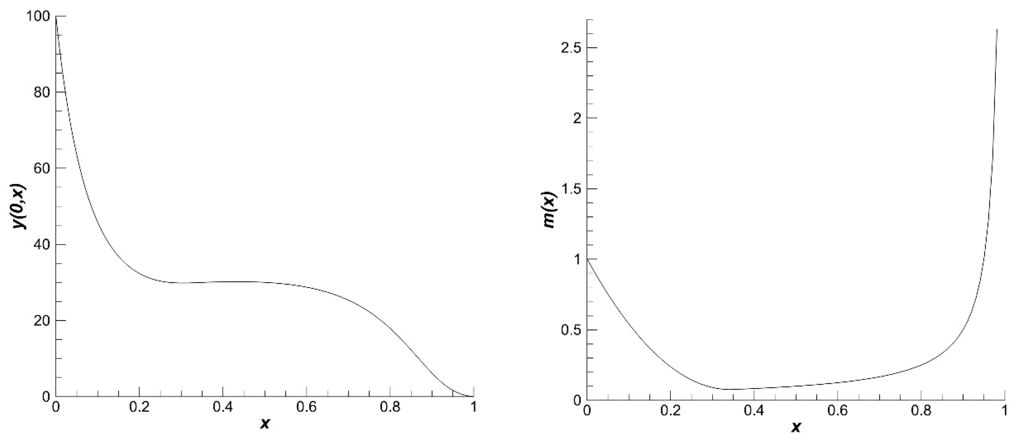
see for example [6,44]. The other parameters of the population are constant and obtained from these formulas and Equation (23). The equilibrium distribution of the size of individuals in population assumes a traditional form (Figure 1, left) [45]. Function $m\left(x\right)$ is defined based on this equilibrium distribution. This function has the form (Figure 1, right)

$$m\left(x\right)=m_0{m}_1\left(x\right) \mathrm{with} m_1\left(x\right)={\left(1+\delta \right)}^{-1} ({\left(1-\frac{x}{x_0}\right)}^2 \theta \left(x_0-x\right)+\frac{\delta }{1-x})$$

(27)

A function $\theta \left(x\right)$ is the Heaviside function [4] and $x_0$ is a fish size at the entry into puberty.

Parameters of the maximum specific mortality $m_0$ and the maximum growth rate $v_0$ are defined from the postulated equilibrium. The age limit ${\tau }_m$ is fixed for a concrete population. Parameter α of the growth rate function is defined from the condition $x\left(\tau \right)\to 1.0$ as $\tau \to {\tau }_m$. Coefficient k of the growth dispersion of the individuals has a small positive value.

3.3. Model without Diffusion

The knowledge of some properties of solutions in the model (24) with used functions of type (25)–(27) is necessary for the adequate application of numerical methods. These properties are studied in the case of control absent (u ≡ 0) for constant conditions of the environment and without diffusion. We have the model

$${\partial }_{t}y+{\partial }_x\left(vy\right)=-m\left(x\right)y^{\gamma }$$

(28)

with the nonlinear functional part.

The Equation (29) is studied in equilibrium case without diffusion. This is an ordinary differential equation:

$$\frac{d\left(vy\right)}{dx}=-m\left(x\right)y^{\gamma }$$

(29)

Proposition 1.

The solution $y\left(x\right)$ of Equation (29) has the property $\underset{x\to 1}{lim} y\left(x\right)=0$ for functions $v, m$ of forms (26) and (27) with positive initial condition.

Proof. 

The function $y\left(x\right)$ is looked for $y\left(0\right)=y_0>0$, $v\left(x\right)$ is of (26). The function of a specific natural mortality rate has form (27).

The solution of Equation (29) defines from the equation ${\left(v\left(x\right)y\left(x\right)\right)}^{1-\gamma }=\left(\gamma -1\right)\left[{{\displaystyle \int }}_0^x\frac{m\left(x\right)}{v^{\gamma }\left(x\right)}dx+c\right]$ with $c=\frac{1}{\left(\gamma -1\right){(v_0{y}_{0 })}^{\gamma -1}}.$ Further transformations result in a formula $v\left(x\right)y\left(x\right)={\left[\left(\gamma -1\right){{\displaystyle \int }}_0^x\frac{m\left(x\right)}{v^{\gamma }\left(x\right)}dx+\frac{1}{{(v_0{y}_{0 })}^{\gamma -1}}\right]}^{-\frac{1}{\gamma -1}}$. Let denote $I_0={{\displaystyle \int }}_0^{x_0}\frac{m_1\left(x\right)}{ v_1^{\gamma }\left(x\right)}dx$, $a_0=\left(\gamma -1\right)\frac{m_0}{v_0}$ then a formula

$$y\left(x\right)=\frac{1}{v_1\left(x\right)}{\left[a_0{I}_0+a_0{{\displaystyle \int }}_{x_0}^x\frac{m_1\left(x\right)}{ v_1^{\gamma }\left(x\right)}dx+\frac{1}{y_{0 }{}^{\gamma -1}}\right]}^{-\frac{1}{\gamma -1}}>0$$

(30)

is obtained for $x\in \left(x_0,1\right)$. A denotation $a_1=a_0{I}_0+\frac{1}{y_{0 }{}^{\gamma -1}}$ gives a formula $y\left(x\right)=\frac{1}{v_1\left(x\right)}{\left[a_1+a_0{{\displaystyle \int }}_{x_0}^x\frac{m_1\left(x\right)}{ v_1^{\gamma }\left(x\right)}dx\right]}^{-\frac{1}{\gamma -1}}$. According to (26) and since $\theta \left(z\right)=0$ for $z\le 0,$ function $m_1\left(x\right)$ for $x\ge x_0$ transforms to $\frac{\delta }{1+\delta } {\left(1-x\right)}^{-1}$. Introducing $a_2=a_0 \frac{\delta }{1+\delta }>0$ and substituting $v_1\left(x\right)={\left(1-x\right)}^{\alpha }$, $m_1\left(x\right)=\frac{\delta }{1+\delta } {\left(1-x\right)}^{-1}$ we obtain $y\left(x\right)=\frac{1}{v_1\left(x\right)}{\left[a_1+a_2{{\displaystyle \int }}_{x_0}^x{\left(1-x\right)}^{-\left(\alpha \gamma +1\right)}dx\right]}^{-\frac{1}{\gamma -1}}>0$.

The integral in the last formula converges and we get the following formulas

$$\begin{array}{l}y\left(x\right)={\left[a_3{\left(1-x\right)}^{\alpha \left(\gamma -1\right)}+\frac{a_2}{\alpha \gamma }{\left(1-x\right)}^{-\alpha }\right]}^{-\frac{1}{\gamma -1}} \mathrm{with} a_3=a_1-\frac{a_2}{\alpha \gamma {\left(1-x_0\right)}^{\alpha \gamma }}. \mathrm{Finally},\\ y\left(x\right)=\frac{{\left(1-x\right)}^{\frac{\alpha }{\gamma -1}}}{{\left[a_3{\left(1-x\right)}^{\alpha \gamma }+\frac{a_2}{\alpha \gamma }\right]}^{\frac{1}{\gamma -1}}}\end{array}$$

(31)

The proof of this proposition follows from the last formula. □

Proposition 2.

The solution $y\left(x\right)$ of Equation (29) has no negative value in set $D$ for functions $v, m$ of forms (26) and (27) with positive initial condition.

Proof. 

Proof of this proposition follows from Formula (30). □

Proposition 3.

The solution $y\left(t,x\right)$ of Equation (28) has property $\underset{x\to 1}{lim} y\left(t,x\right)=0$ for functions $F,v, m$ of forms (25)–(27), and any t with nonnegative initial and boundary conditions.

Proof. 

The method of characteristics is applied to Equation (28). An equation of characteristics has the form

$$c=t-v_{\_}\left(x\right)$$

for any constant c. Here is the formula $v_{-}\left(x\right)={{\displaystyle \int }}_0^x \frac{dx}{v\left(x\right)}$. From this formula follows

$$t\left(x\right)=v_{\_}\left(x\right)+c$$

(32)

on the characteristic. Equation (32) shows that on the characteristic the equation (28) transforms to (29). The completion of the proof is the same as for Proposition 1. □

Proposition 4.

The solution $y\left(t,x\right)$ of Equation (28) has no negative value in set $T\times D$ for functions $F,v, m$ of forms (25)–(27) with positive values of functions in initial and boundary conditions.

Proof. 

Proof has an analogue with proposition 3 proof on the base of the Formula (32). □

3.4. Unstable Environments Characteristics

Usually, the function $y_1\left(t\right)$ is represented as $y_1\left(t\right)={{\displaystyle \int }}_0^{1}b\left(x\right)y\left(t,x\right)dx$. This formula describes a fertility process with birth intensity $b\left(x\right)$. We are modelling a population with a high fertility intensity and a high death rate at early ontogenesis. A population of fish can serve as an example. Recruit groups have quasi-stochastic abundance. We simulate this fact as a function $y_1\left(t\right)$. It is assumed that there is no stock-recruitment relationship in the population. We use a scenario imitating the annual birth rate changes under the influence of climate and seasonal variations. The birth rate function is expressed as

$$y_1\left(t\right)={\epsilon }_{\left[t\right]}{y}_0\left(0\right)\left(1+sin\frac{4\pi t}{T}\right)\psi \left(t\right)$$

(33)

The constant $y_0\left(0\right)$ characterizes some average level of a spawning intensity. The influence of the evolutionary dynamics of the environment is described as $\left(1+sin\frac{4\pi t}{T}\right)$. The planning horizon T has twice the period. Symbols [t] and $\left\{t\right\}$ designate integer and fractional parts of number t correspondingly. Function $\psi \left(t\right)=b_0{\left\{t\right\}}^2{\left(1-\left\{t\right\}\right)}^4$ describes the seasonal dynamics of the spawning intensity. Parameter $b_0=3^6/2^4$ is a normalizing multiplier. The maximum of the function $\psi \left(t\right)$ is 1. The indexes of degrees of this function are defined from the condition of the maximum of the spawning intensity in the first half of every year. Parameter ${\epsilon }_{\left[t\right]}$ denotes a level of spawning intensity relative to $y_0\left(0\right)$. This parameter describes random changes in the environment. It is constant for one calendar year. For every year it is a random variable ε distributed on the interval $\left[0,{\epsilon }_{\max }\right]$ with a probability density

$$\left\{\begin{array}{cc}\frac{2}{{\epsilon }_{\max }}\epsilon ,& \epsilon \in \left[0,1\right]\\ \frac{2}{{\epsilon }_{\max }\left({\epsilon }_{\max }-1\right)}\left({\epsilon }_{\max }-\epsilon \right),& \epsilon \in \left[1,{\epsilon }_{\max }\right]\end{array}\right.$$

(34)

and describes the random influence of the environment on the birth rate. The parameter ${\epsilon }_{\max }$ has a value greater than unity. The function $y_1\left(t\right)$ is a smooth function.

The traditional relation “stock-recruitment” is not used because the fish have an extremely high production of roe during spawning and extremely high mortality of individuals at the stage of development from roe to larvae and small fish. This mortality is caused by the strong influence of the environment in spawning places. This influence is variable and indicates that the spawning efficiency is frequently defined by random factors of habitat conditions, rather than the number of parents. Such a situation is typical for many fish species. Our model description is focused on such species of fish.

A scenario is based on this condition (33) and (34). This is presented in Figure 2.

Zero age corresponds to age 0+ of a young fish in our model. Condition $y_2\left(t\right)=0$ (see Formula (24)) conforms to the natural mortality function (Figure 1). The growth rate has a nonlinear dependence on the size as $\alpha <1$ [6]. The dependence of natural mortality on population density is also nonlinear since $\gamma >1$ [46]. The diffusion coefficient corresponds to the concept of weak dispersion of growth rate. The modelling period was taken to be twice the age limit $T=2{\tau }_m$.

3.5. Parameters of Fishery

The mortality function taking into account natural mortality, fishery, and seasonal effects has the following form:

$$F\left(t,x,y,u\right)=-m\left(x\right)y^{\gamma }-q\left(x\right)u\left(t,x\right)\psi \left(t\right)y$$

(35)

The function of the income from fishery has a nonlinear dependence on fishing effort $u\left(t,x\right)$ [7].

$$\phi \left(t,x,y,u\right)=p\left(x\right)q\left(x\right)u\left(t,x\right)\psi \left(t\right)y-c\left(x\right)u^2\left(t,x\right)$$

(36)

Function q(x) of catchability has form $q\left(x\right)=q_{0 }\theta \left(x-x_0\right)$ where $\theta \left(x\right)$ is the Heaviside function [4]. At the same time, the catchability coefficient is taken to be equal to the maximum natural mortality $q_0=m_0$. This condition is a model assumption. The function of the income from the fishery is a piecewise linear function $p\left(x\right)=p_{0 }\frac{1-x}{1-x_0}\theta \left(x-x_0\right)$. The parameter $p_{0 }$ is the highest specific income from harvesting individuals of size $x_0$. As the size increases, the income decreases. These two functions describe a situation in which fishery is conducted in spawning places, where harvesting is allowed only for mature fish. In practice, this condition is often satisfied for pelagic fish [6].

The cost function of fishery intensity is chosen to be constant $c\left(x\right)=c_0$. The intensity function depends only on time $u\left(t,x\right)\equiv u\left(t\right)$. This condition corresponds to the real situation of the fishery, where only quantitative but not qualitative operational changes of fishery gear are possible. The differentiation of fishery efforts according to the size of individuals means the qualitative change of fishery gear, which cannot be done promptly. In our model, these properties of fishery gear are described by a catchability function.

3.6. Numerical Method

The main difficulty in finding numerical solution of Euler-Lagrange equations (problem (1)–(5)) is that equation for $y\left(t,x\right)$ must be solved forward in time, while Equation (5) for adjoint function $\lambda \left(t,x\right)$ must be solved backward in time. Therefore, the optimal harvesting rate was computed by a direct method. The Equations (1)–(3) were discretized on a regular grid in $T\times D$ and optimization criterion (3) was treated as a nonlinear optimization problem with respect to the values $u(t_j)$ of control function on discrete grid points. For given values of $u(t_j)$ the solution of Equations (1) and (2) was computed by the Crank-Nicolson method.

Previous constructions of model parameter relationships have led us to determine the numerical characteristics of an example that we consider to be characteristic of pelagic fish (

Table 1. Model parameters.

Parameter	Description	Value
$y_0$	Initial population density of zero-sized individuals	102
$x_0$	Size at the entry into puberty	0.35
$\alpha$	Growth rate parameter	0.83
$\mathsf{\gamma }$	Parameter of the specific mortality function	1.1
$k$	Diffusion coefficient	0.001
${\epsilon }_{\max }$	Parameter of birthrate variation	10
${\tau }_m$	Maximum longevity	25
$q_0$$, m_0$	Catchability coefficient and maximum natural mortality	1.82
$p_0$	Parameter of catchability function	4.0
$v_0$	Parameter of the speed of growth function	0.24

). These are species as pollack, herring, saury, sardine, and other similar species [7,17,45].

4. Results

Let us now consider the model with harvesting. It is model (24) with functions from Section 3. The recruitment dynamics, which are determined by the environment, play a major part in our calculations. Different scenarios of environment variations result in different scenarios of recruitment dynamics. We have chosen a scenario based on Equations (20)–(22), which is shown in Figure 2. 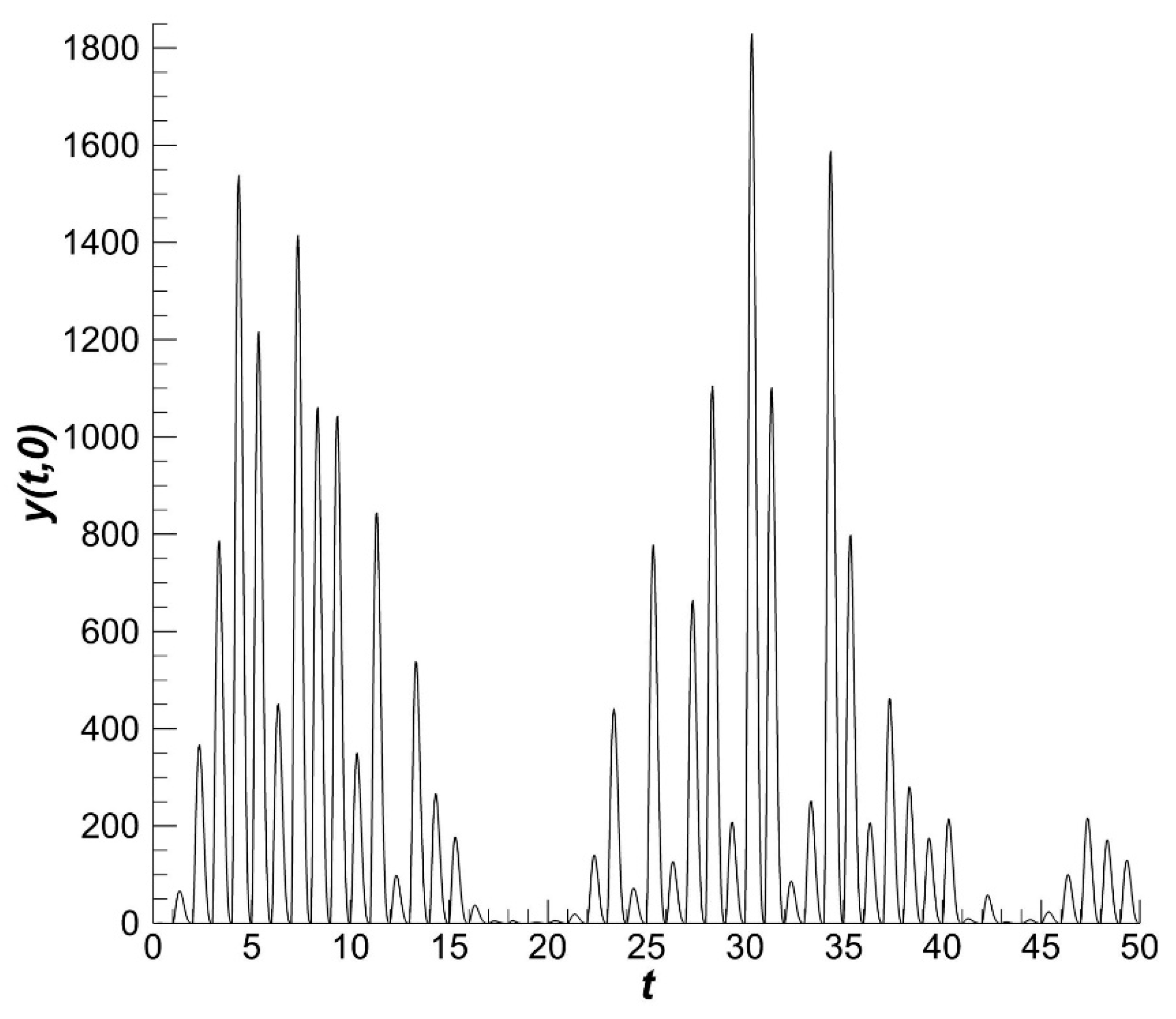This scenario is typical for many pelagic and semi-pelagic fish species in unstable environments [47]. The corresponding dynamics of population density in the case of zero harvesting is shown in Figure 3.

The population density varies from generation to generation that is formed under the influence of the environment which is crucial in the stage of larvae (see Formulas (33)–(36)). The gradients of population density are less pronounced than the gradients of recruitment. We will see later that it is true irrespective of the presence of harvesting.

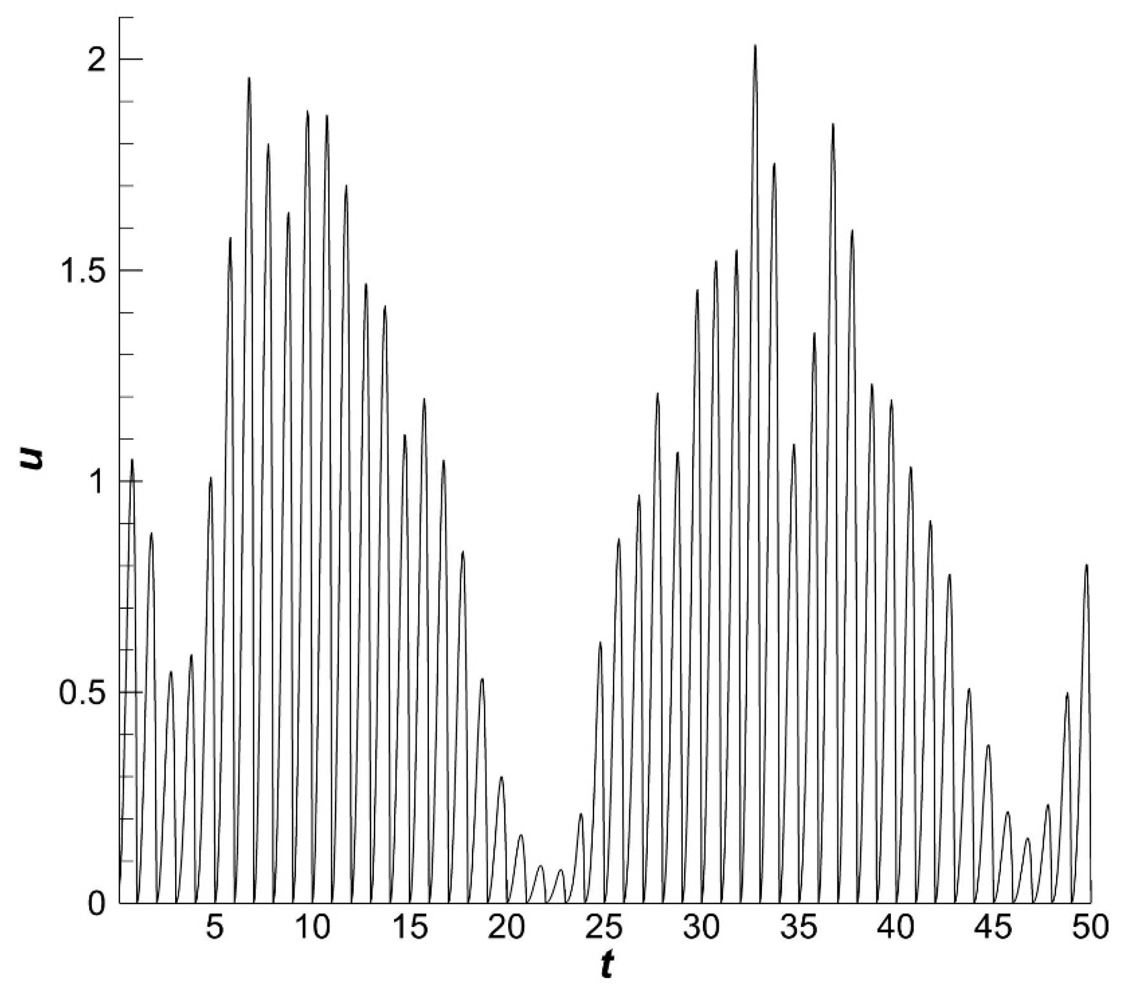
The dynamics of the optimal fishing effort $u\left(t\right)$ is characterized by high rates (Figure 4).

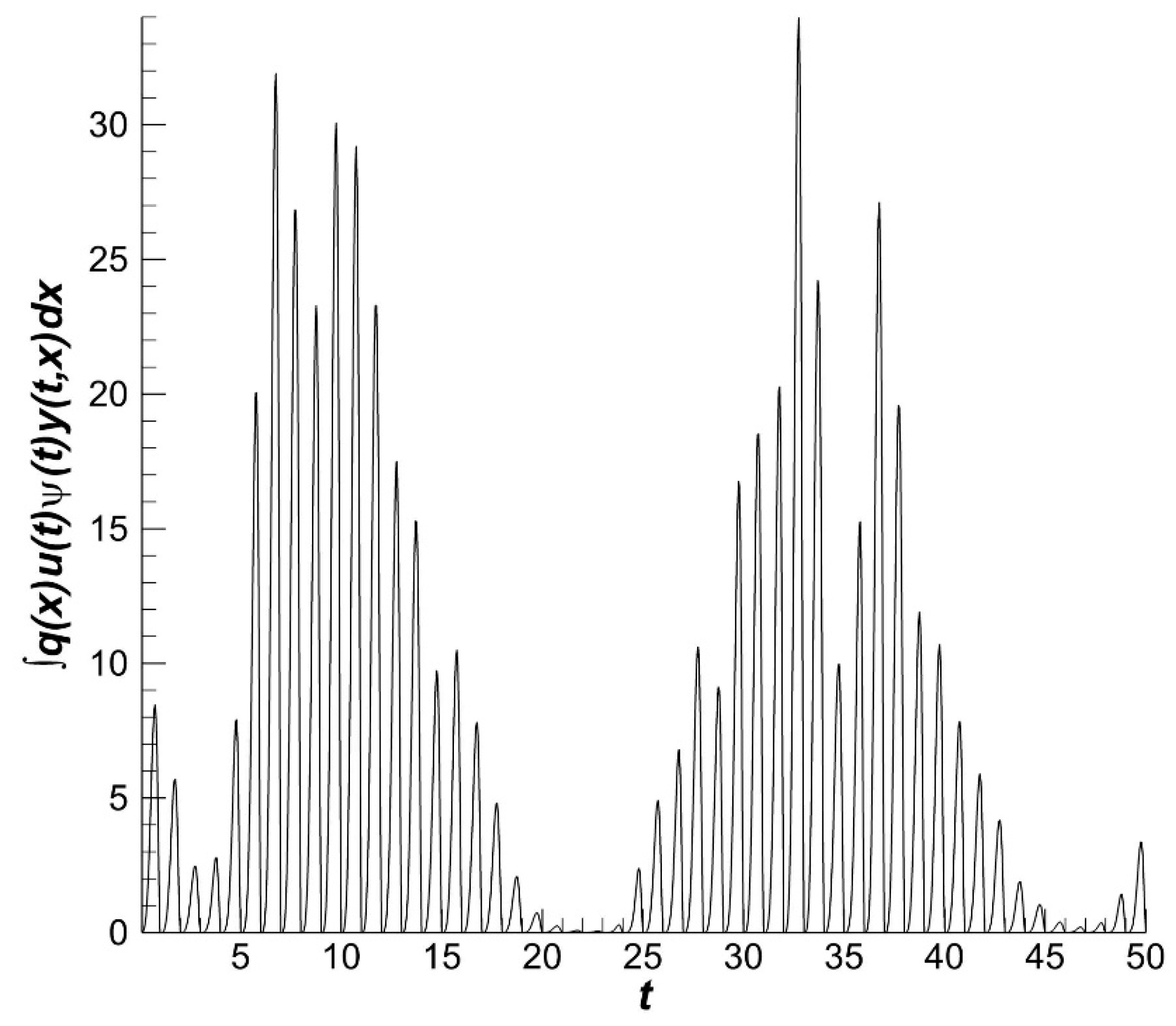
The result of harvesting is the catch volume for a particular time interval. In our consideration, the time interval is 50 years (Figure 5). The gradients of the catch volume dynamics are less pronounced than the gradients of fishery intensity. The catch result depends on the population conditions and the properties of fishery gear. The gear is constructed to obtain the maximum harvest income and to comply with fishery rules. Fish are harvested when they are sexually mature. This requirement indicates that fish to be harvested must have a size greater than some fixed size $x_0$ (see Section 3).

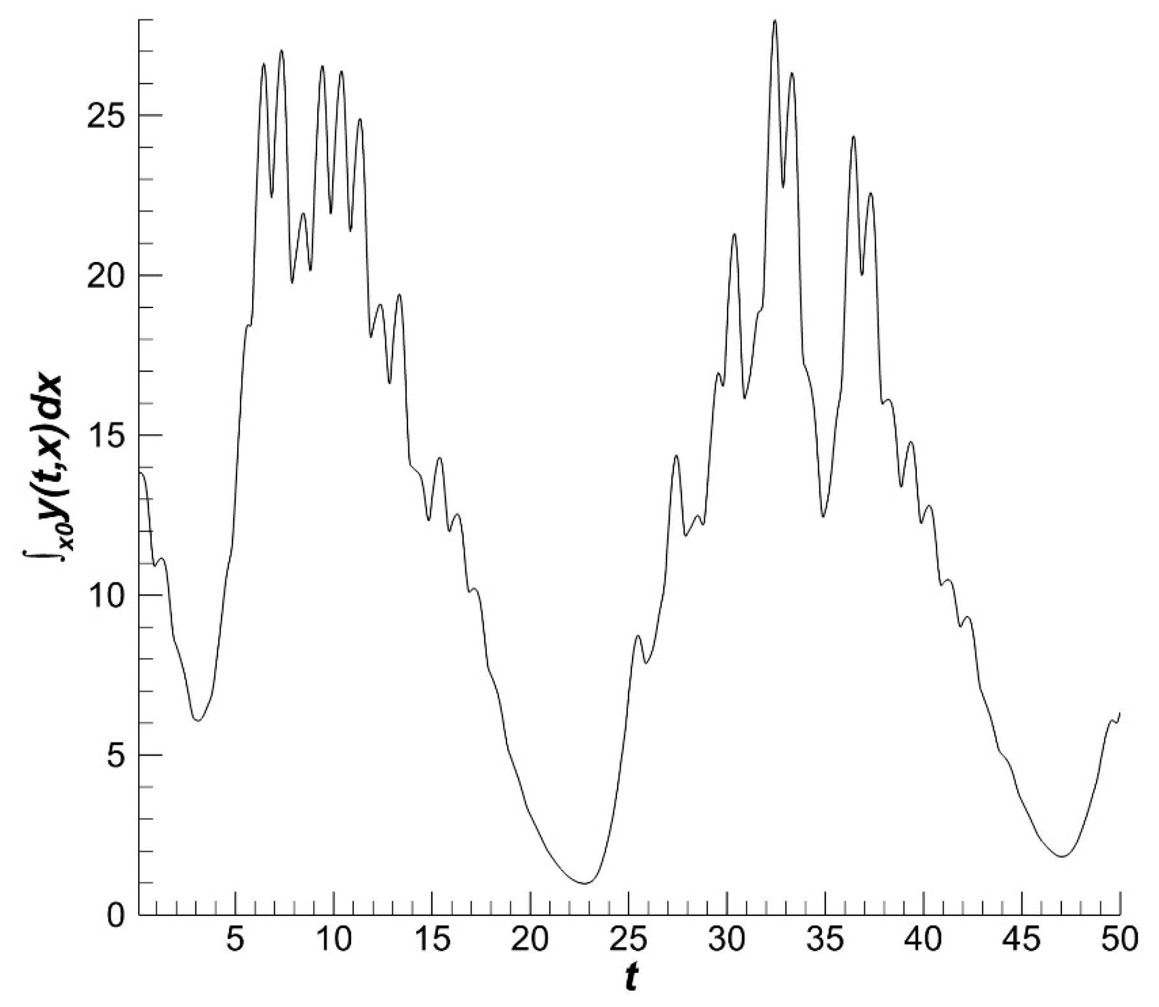
The fishery part of the population and catch volume have similar dynamics (Figure 5 and Figure 6). The influence of the environment on the population as a whole is smaller than its influence on recruitment.

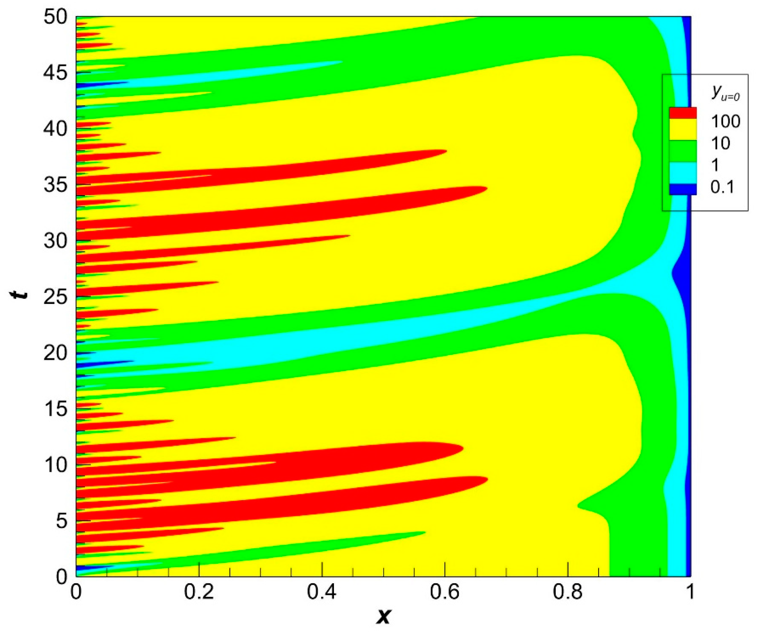
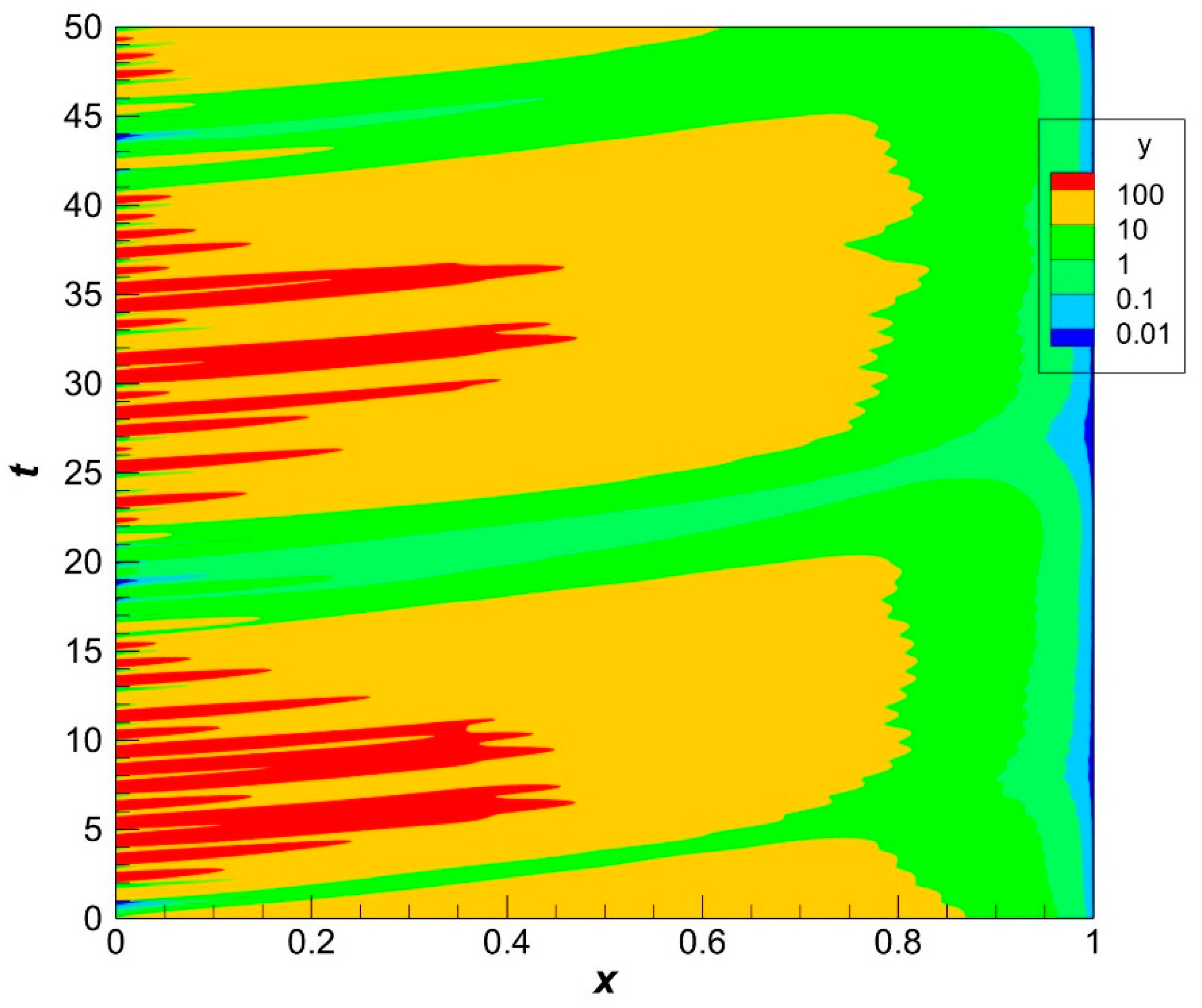
The population dynamics have smaller gradients than the recruitment dynamics. The population density under the influence of fishery is smaller than that without fishery. The fishery decreases the average size of individuals. The density fluctuations under fishery have a smaller amplitude than without fishery (Figure 7). These conclusions may be given based on a qualitative comparison of results in Figure 3 and Figure 7.

The nonlinear dependence of income function (see Formula (36)) on fishery effort cardinally changes the properties of control function u(t). In the classical linear case, the control function u(t) is a discontinuous function [5]. The implementation of this function in the fishery process is difficult. Whereas for nonlinear income control function u(t) is continuous and can be easily implemented in a real fishery process.

5. Discussion

The above results enable us to derive the following conclusions. Our research and results are in line with similar work on the effects of population structures on viability under anthropogenic influences and habitat changes. More specifically, we are talking about the effects of fishing on fish populations. Various authors (e.g., [10,11,12,13,20] in our list of references) have examined the functioning of fish populations when age or size structures are factored into models. In these studies, general patterns of construction of optimal modes of fishing were revealed. In our model study, we are focused on the commercial population of pelagic fish. These are fish species: pollock, herring, saury, sardine, and others like them [7,17,45,47]. These fish species live in the upper layers of marine and ocean waters, actively move, spawn in certain places and at certain times. During spawning, they form dense aggregations and are fished at this time. The latter feature is the basis of our constructions of the catchability function q(x), the fishery rate and fishery income functions (Section 3.5).

We have also complemented the existing studies by considering the conditions of habitat variability that directly affect the occurrence of large or small generations in a population. This is the novelty of our research in modelling the dynamics of fish populations. The main result is the model-detected effect of increasing population resilience through size structuring. An optimal fishing regime enhances population stability. Conclusions are made on the basis of qualitative comparison of our results with in situ observations and model results of other authors [6,7,8,9,10,11,12,13,15,16,18,19,47].