aSGD: Stochastic Gradient Descent with Adaptive Batch Size for Every Parameter

Abstract

In recent years, deep neural networks (DNN) have been widely used in many fields. Lots of effort has been put into training due to their numerous parameters in a deep network. Some complex optimizers with many hyperparameters have been utilized to accelerate the process of network training and improve its generalization ability. It often is a trial-and-error process to tune these hyperparameters in a complex optimizer. In this paper, we analyze the different roles of training samples on a parameter update, visually, and find that a training sample contributes differently to the parameter update. Furthermore, we present a variant of the batch stochastic gradient decedent for a neural network using the ReLU as the activation function in the hidden layers, which is called adaptive stochastic gradient descent (aSGD). Different from the existing methods, it calculates the adaptive batch size for each parameter in the model and uses the mean effective gradient as the actual gradient for parameter updates. Experimental results over MNIST show that aSGD can speed up the optimization process of DNN and achieve higher accuracy without extra hyperparameters. Experimental results over synthetic datasets show that it can find redundant nodes effectively, which is helpful for model compression.

1. Introduction

In recent years, as the hottest branch of machine learning, deep learning has been playing an important role in our production and life. Due to its significant advantages over traditional machine learning algorithms, deep learning has excellent performance in areas such as image classification [1], speech recognition [2], cancer diagnosis [3,4], rainfall forecast [5,6,7], and self-driving cars [8,9]. A deep neural network (DNN) is a kind of deep learning technique that was initially designed to function like the human nervous system and the structure of the brain. Compared to the earlier shallow networks, DNN consists of multiple layer of nodes, including input, hidden and output layers. The nodes of each layer are connected to the nodes of the adjacent layers by weights, and each node has an activation function. Most of the activation functions are nonlinear, such as sigmoid [10], ReLU [11], and tanh [12]. The inputs are multiplied by their respective weights and summed at each node, and the sum is transformed via an activation function. The output of the activation function is then fed as input to the node in the next layer. This process continues until the output layer is reached. The final output is processed by other methods to solve real-world problems. In order to achieve the right output, the parameters of the DNN need to be optimized. The DNN comprises complicated functions with lots of nonlinear transformations, so most optimization functions are non-convex functions with local optima and global optima. Many optimization methods can be used to find the optimal parameters, including backpropagation (BP) algorithms [13], Markov chain Monte Carlo (MCMC) algorithms [14], evolutionary algorithms [15], and reinforcement learning [16]. MCMC algorithms are a class of sampling algorithms used to obtain a sequence of random samples from a probability distribution. They work by constructing a Markov chain with an equilibrium distribution equal to the target probability distribution. It may require sampling many times to make the sample match the target distribution, but it helps to find the global optima. The BP algorithm is the most commonly used in deep learning, also known as the gradient descent method. It is a very classic algorithm to find the local minimum of an objective function by taking repeated steps in the opposite direction of the gradient of the function at the current point [17]. The rapid development of deep learning is partly due to the continuous improvement of optimization algorithms. Many improved optimization algorithms based on gradient have been proposed [17]. It started with three gradient descent variants: batch gradient descent, stochastic gradient descent, and mini-batch gradient descent. The difference between them lies in the number of samples used to calculate the gradient of the objective function. Due to two problems, the mini-batch gradient descent does not guarantee good convergence. First is the saddle point [18]. Since the gradient in all dimensions around the saddle point is close to zero, it is difficult for the mini-batch gradient descent to escape. Second is an appropriate learning rate. A too-small learning rate will lead to slow convergence, while a too-large learning rate will hinder convergence. The same learning rate applies to all parameter updates in the mini-batch gradient descent, but differences between samples and features with different frequencies require a larger update in specific parameters for rarely occurring features.

Momentum [19] is a method that helps mini-batch gradient descent to escape the local optima or the saddle point. By adding a portion of the past updated gradient to the present gradient, it accelerates training and also reduces oscillations of loss. In addition, an adaptive learning rate is also a way to accelerate training. Adagrad [20] is an algorithm based on an adaptive learning rate. By using a different learning rate for every parameter depending on their past gradients, Adagrad performs larger or smaller updates to each individual parameter. Adagrad divides the learning rate by the accumulation of the squared past gradients when updating the parameters. This makes the learning rate continually decrease, even to an infinitesimally small size. To solve this problem, Adadelta [21] limits the window of accumulated past gradients to a fixed size, instead of accumulating all past squared gradients in Adagrad. The RMSprop [22] is another algorithm for solving the continued decline in learning rates. The learning rate in RMSprop will divide by an exponentially decaying average of squared gradients. Adam [23] is another method that combines an adaptive learning rate and momentum. Adam stores an exponentially decaying average of past squared gradients, such as Adadelta and RMSprop, for the adaptive learning rate, and it keeps an exponentially decaying average of past gradients for momentum.

These algorithms are very effective in improving model training, but they also introduce more hyperparameters. Adjusting these hyperparameters is based on data and training. It takes a lot of time for trial and error, which has certain requirements for the user’s ability [24]. Furthermore, the above optimizers mainly focus on improving the convergence rate (adaptive learning rate). They care about the information from previous parameter updates. Regarding the impact of samples on model training, the research is mainly focused on selecting an appropriate batch size [25,26] or strategy for selecting samples [27,28,29]. However, little attention has been paid to the subtle distinction of the impact of a sample on different parameters. Additionally, owing to the improvement in the storage and computing capabilities of current computers, the development of GPUs and TPUs has ensured the speed of model training and the depth of the network structure. However, deeper networks are often more difficult to train [30], so it is a problem to design a suitable network structure based on the complexity of the task [31]. In order to complete complex tasks, some deep neural networks (DNN) often set the number of layers to hundreds or even deeper, and it is difficult to know whether there are redundant nodes.

In the paper, we analyzed the role of samples in the parameter update and found that each of the training samples in the same batch might play a unique role in updating. That means the effects of samples on parameter updates vary greatly. We can use such differences to update the parameters in a novel manner. In order to maximize this difference, we take ReLU [32] as the default activation function. It directly changes the degree of this effect into whether or not there is an effect. Based on this observation, we proposed sample-based adaptive batch size gradient descent (aSGD), which is a variant of the gradient descent method. Without additional hyperparameters, it can speed up the optimization process of the DNN and achieve higher accuracy than SGD. In addition, it could help one discover redundant nodes in a neural network.

The remainder of this paper is organized as follows. In Section 2, we visualize the effect of samples on parameter updating and present the proposed method, i.e., aSGD. In Section 3, we demonstrate the properties of aSGD using three experiments. The conclusion is drawn in Section 4.

2. Materials and Methods

2.1. Gradient Descent

Gradient descent is a common optimization algorithm for finding a local minimum of a differentiable function. It is often used to optimize parameters in machine learning. Most optimization problems of machine learning can be considered as minimizing a cost function. Such a function is called the objective function. By iteratively updating the parameters in the reverse direction of the gradient (i.e., the vector containing all the partial derivatives of the objective function), we can continuously reduce the value of the target function to approach the local minima.

The objective function used by a machine learning algorithm often decomposes as an expectation of the per-samples loss function (e.g., mean squared error loss, and cross-entropy loss) overall training samples

$$L(x,y,\theta )=\frac{1}{M}\sum _{i=1}^{M}l\left(x^{\left(i\right)},y^{\left(i\right)},\theta \right)$$

(1)

where L is the expectation of the loss function, $\left\{(x^{\left(1\right)},y^{\left(1\right)}),(x^{\left(2\right)},y^{\left(2\right)})\dots ,(x^{\left(M\right)},y^{\left(M\right)})\right\}$ is the training data, $\theta$ represents training parameters, l is the pre-sample loss, and M is the size of the training data.

To minimize such an objective function, the gradient descent needs for computing

$$g=\frac{1}{M}\sum _{i=1}^M{\nabla }_{\theta }l\left(x^{\left(i\right)},y^{\left(i\right)},\theta \right)$$

(2)

where g is the mean gradient of this overall loss, and ${\nabla }_{\theta }l$ is the gradients of the individual sample. The computational cost of Equation (2) is $O\left(M\right)$. If the size of the training set is large, it will take a significant amount of time for one calculation.

The stochastic gradient descent (SGD) was proposed to solve the expensive computational cost. The main idea of SGD is that the expected losses over the overall training set (i.e., $L(x,y,\theta )$ in Equation (1)) can be approximately estimated by using a mini-batch of training samples. Algorithm 1 shows how to estimate expected loss and its gradients. m is fixed, even if the training set size M grows. So, the cost of each parameter update does not directly depend on the training set size M, and the computational cost of SGD is $O\left(m\right)$.

In addition, those methods that use more than one but fewer than all the training samples were traditionally called mini-batch or mini-batch stochastic methods, and it is now common to call them simply stochastic methods [33].

Algorithm 1: Stochastic gradient descent

2.2. The Role of Samples in Parameter Updating

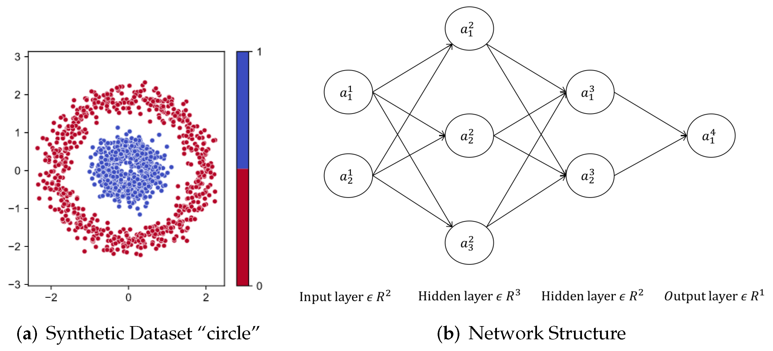
It can be found that the optimization problems can be considered as minimizing the expectation of the per-sample loss function over all training samples. SGD uses a small set of samples to estimate this expectation. The overall loss is the mean of the losses of the instances in this batch; then, the gradient of this overall loss is the mean of the gradients of the individual losses.

However, it can be seen from line 3 in Algorithm 1 the expectation derived from the accumulation of samples. The information in each sample is different, so the effect of each instance on any parameter in the model varies greatly. That is, both the partial derivatives of a single sample loss on different parameters and the partial derivatives of per-sample loss to the same parameter are very multifarious. So, there are some partial derivatives in a gradient that are negligible. When we use ReLU as an activation function, it will come to 0. We show this through a practical example for better understanding.

2.2.1. Notations

As shown in Figure 1a, the “concentric circle” data are used as a binary classification example to reveal the different role of each sample in the parameter update. It is a binary classification problem with coordinates as input and categories as output. The inner blue points are regarded as a “positive class”, and the outer red points are regarded as a “negative class”. The data are trained through a fully connected network with one input layer, two hidden layers, and one output layer. The ReLU is used as an activation function of neurons in hidden layers. We make notational conventions for the convenience of description. The four layers in Figure 1b are denoted by L1, L2, L3, and L4, respectively.

Backpropagation is gradient descent applied to deep learning. The equations of backpropagation are shown in Equations (3)–(6), respectively. The total number of layers is L. The “error” of the j-th neuron in the l-th layer is ${\delta }_j^l$, and ${\delta }^l$ is the “error” vector of neurons in layer l. ${\nabla }_{a}C$ is defined as a vector whose components are the partial derivatives $\partial C/\partial a_j^l$, and the cost function is C. $a_j^l$ is the activation of the j-th neuron in the l-th layer. ⊙ denotes the element-wise product of the two vectors, namely the Hadamard product. $z_j^l$ is the weighted input to the j-th neurons in layer l, and $z^l$ is the weighted input vector of neurons in layer l. $\sigma$ denotes this kind of element-wise application of the activation function, and ${\sigma }^{\prime }$ is the derivative of the activation function. T represents the transpose of the matrix. The $w_{jk}^l$ is used to denote the weight for the connection from the k-th neuron in the $(l-1)$-th layer to the j-th neuron in the l-th layer and the weight coefficient matrix (matrix consisting of $w_{jk}^l$) of neurons in layer l is $w^l$. $b_j^l$ is the bias of the j-th neuron in the l-th layer.

For a neural network, the “error” in the output layer can be derived from the cost, activation and weighted input by Equation (3), and then propagated to other hidden layers by Equation (4). The gradient can be derived from the error and activation by Equations (5) and (6). The gradient of the cost function can be quickly found by the backpropagation algorithm. Thus, the parameters of the neural network are solved iteratively using gradient descent.

$${\delta }^L={\nabla }_{a}C\odot {\sigma }^{\prime }\left(z^L\right)$$

(3)

$${\delta }^l=\left({\left(w^{l+1}\right)}^T{\delta }^{l+1}\right)\odot {\sigma }^{\prime }\left(z^l\right)$$

(4)

$$\frac{\partial C}{\partial b_j^l}={\delta }_j^l$$

(5)

$$\frac{\partial C}{\partial w_{jk}^l}=a_k^{l-1}{\delta }_j^l$$

(6)

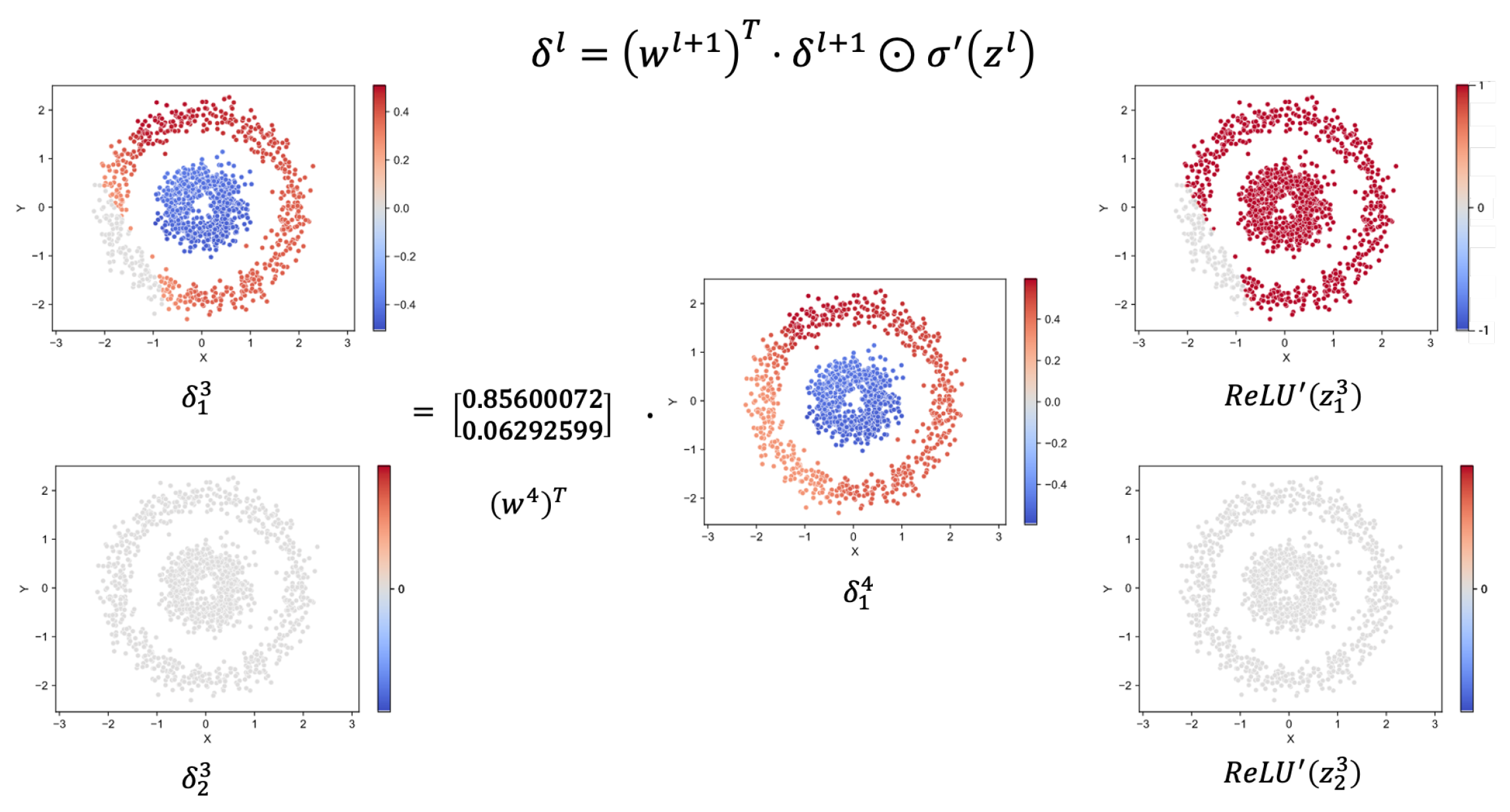
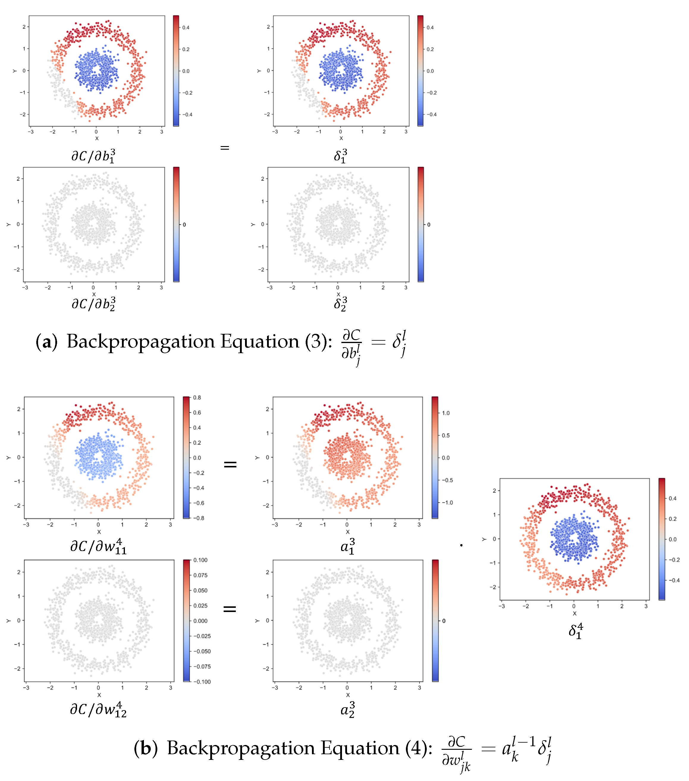
2.2.2. Back Propagation Visualization

It can be seen from Equation (4) that the “error” of any hidden layer node is calculated by two parts, $\left({\left(w^{l+1}\right)}^T{\delta }^{l+1}\right)$ and ${\sigma }^{\prime }\left(z^l\right)$. The derivative function of the ReLU is given by

$${ReLU}^{\prime }\left(x\right)=\left\{\begin{array}{cc}1\hfill & \mathrm{if}x>0\hfill \\ 0\hfill & \mathrm{if}x\le 0\hfill \end{array}\right.$$

(7)

${ReLU}^{\prime }\left(x\right)$ divides all of samples with $\left({\left(w^{l+1}\right)}^T{\delta }^{l+1}\right)$ into two parts due to the positive or negative $z^l$. The part greater than 0 is kept, and the rest is changed to 0. As a result, the ${\delta }^l$ comes to 0. Such a phenomenon has two effects:

First, the “error” no longer propagates. It can be seen from Equation (4) that for the samples with 0 “errors” in this layer, their “errors” in the next layer also become 0. Consequently, their errors can no longer propagate to the next layer, exacerbating this phenomenon. We visualized each factor term in Equation (4) when $\delta$ passes from L4 to L3 in Figure 2.

The second is that the estimation of the gradient is biased. It can be seen from Equations (5) and (6) that the gradient is related to the “error”. When ${\delta }^l=0$, the $\partial C/\partial w_{jk}^l$ and $\partial C/\partial b_j^l$ are both 0, and the estimation of the gradient is biased. It should be noted that $\partial C/\partial w_{jk}^l$ also contains the ReLU function. In other words, even if ${\delta }^l\ne 0$ and it can be propagated to this layer, the estimation of gradient is biased for $a^l=0$. As for Equation (4), we also visualized Equations (5) and (6) in Figure 3.

2.2.3. Dummy Node

It is worth mentioning that there is such a node that is suppressed for the input of every sample, such as $a_2^3$ in Figure 3b. We define it as follows: for any sample, the $\sigma \left(z^l\right)<0$, such a node is called the true dummy node. On the contrary, if a node is activated for all samples, that is, for any sample, the activation $\sigma \left(z^l\right)>0$, which is called the pseudo dummy node. Both of them are called dummy nodes.

It can be seen from $a_2^3$ in Figure 3b that inputs of all samples in true dummy node are suppressed. Its outputs are 0, which has no effect on the final classification result. In addition, it can be seen from Equations (4) and (6) that true dummy nodes will seriously hinder the propagation of “errors” and the updating of their own parameters. So, true dummy nodes can be regarded as redundant nodes in the model [34].

Here, we only visualize the backpropagation process between L3 and L4. This phenomenon also exists in other hidden layers. Through Figure 2 and Figure 3, we can intuitively see how multiple samples affect the update of the same parameter and the effects of one sample on the update of different parameters.

2.3. Sample-Based Adaptive Batch Size Gradient Descent

As shown in lines 3 and 4 of Algorithm 1, the expected losses over the overall training set are estimated by using a mini-batch of training samples, and then the gradient is calculated from the mean of each gradient of the individual samples ($g={\nabla }_{\theta }L(x,y,{\theta }_t)=\frac{1}{m}{\sum }_{i=1}^m{\nabla }_{\theta }l\left(x^{\left(i\right)},y^{\left(i\right)},\theta \right)$). However, based on the visualization results in Section 2.2.2, the contribution of each sample to the same parameter update is unique (each point in Figure 3 has its own value). With the property of activation function ReLU, some samples do not even contribute to the parameter update because their “errors” no longer propagate in the backward propagation (gray dots in Figure 2), and the gradient disappears (gray dots in Figure 3). This results in a deviation in the gradient estimation of SGD. Some samples in the mini-batch do not contribute to parameter update, but still count as valid samples when calculating the expectations. It results in the batch size (m in Algorithm 1 line 3) being overestimated, and the expected gradient over the overall training set is underestimated. Therefore, we propose a sample-based adaptive batch size gradient descent (aSGD), which estimates the loss and gradient separately for each parameter in the model.

As shown in Algorithm 2, by making a non-zero judgment ($r\left(x\right)$) on the calculated gradient of each sample and summing them up, we can obtain the number of samples that really influence the update parameters and make an estimate on these samples. We call the number of samples adaptive batch size ($m_j^l$ in Algorithm 2 line 4), and the estimated gradient is called the mean effective gradient ($g\left({\theta }_{tj}^l\right)$ in Algorithm 2 line 5).

The problem of SGD underestimating the gradients is solved in aSGD. The expected gradient over the overall training set is accurately estimated by the mean effective gradient. In addition, due to the variability of the samples, each parameter in the model has its own adaptive batch size and mean effective gradient. It makes aSGD an adaptive method and becomes more accurate and effective.

The calculating adaptive batch size is added to aSGD in line 4 of Algorithm 2, so the time complexity of aSGD is $O\left(2m\right)$ and can be approximated as $O\left(m\right)$. In practical application, the per-samples loss in one batch makes up a tensor, so only one calculation is required. All operations on them are vectorized, it will not cause an increase in training time.

Algorithm 2: Sample-based adaptive batch size gradient descent

3. Experiments

In this section, three experiments are conducted to reveal the characteristics of the proposed method. Experiment 1 uses the same network structure and training data as in Section 2. We recorded the changes in all parameters during the entire model training process and analyzed the effect of aSGD on the training process. In Experiment 2, we adopted a new network structure and two synthetic datasets and counted the step, accuracy, and loss when the training was complete for comparing the effect of aSGD and SGD on the neural network and training results. In Experiment 3, we used the MNIST handwritten digit database to test the performance of aSGD and SGD, and repeated the experiment 100 times and counted the results.

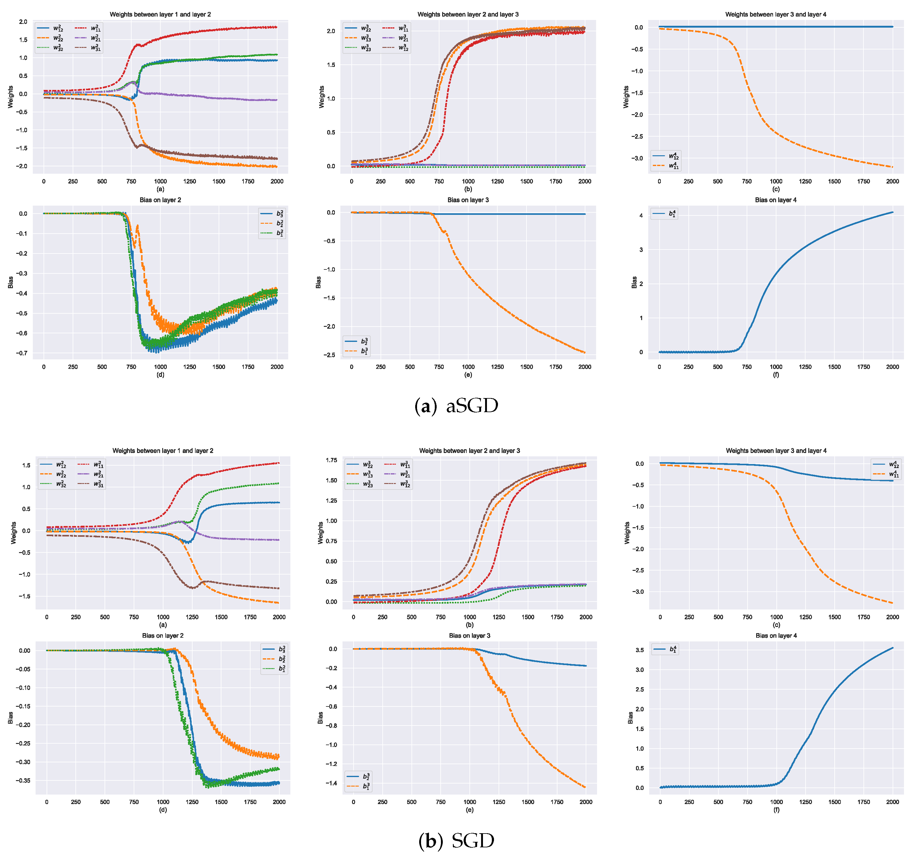
3.1. Properties of aSGD

We trained the same network in the second section with aSGD and SGD, respectively. The update of parameters during the entire training process is shown in Figure 4. By comparing the variation of parameters under the two optimizers, we found two properties of aSGD.

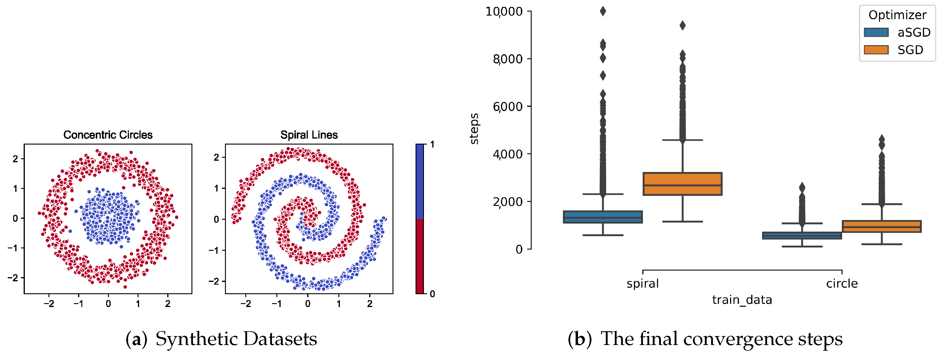
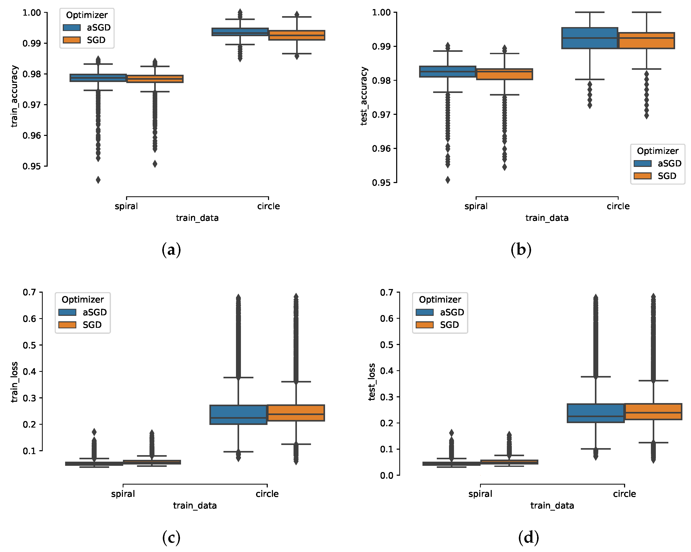
3.1.1. Accelerating Training Process

Comparing the parameter change curves under the two optimizers, such as $w_{11}^3$, $w_{12}^3$, $w_{13}^3$ and $b_1^3$, it is easy to find that the range and rate of the change of parameters in aSGD are greater than SGD. This is because aSGD uses the mean effective gradient defined in Section 2 as the actual gradient for parameter updates. Compared with the gradient in SGD, the mean effective gradient will be larger in a single step. This is due to the adaptive batch size that corrects the biased estimation of the overall gradient in SGD caused by the ReLU function. It makes the expected gradients over the overall training set well estimated by the mean effective gradient. The gradient descent method becomes more effective and accelerates the training process.

The adaptive batch size is similar to the adaptive learning rate, but the basis of the two adaptations is very different. Such adaptive learning rate methods as Adagrad, Adadelta, RMSprop, and Adam accumulate the gradient in a range of time steps to adjust the learning rate dynamically. This results in a proper gradient for each parameter, and the model will converge faster. A proper gradient comes from samples in aSGD. The differences between the samples and features with different frequencies make the gradient of each parameter varied. Each time the parameters are updated, the mean effective gradient is accumulated from several samples. This adaptation is reflected in the adaptive batch size. In other words, the adaptive learning rate takes advantage of the difference caused by the change in the parameter during the training process, and the adaptive batch size takes advantage of the difference in parameters caused by samples in one batch. However, this difference can only be due to the specific activation characteristic of the ReLU. Specially, the ReLU will return 0 when the value of the linear activation is less than 0. Consequently, theses samples do not contribute to the parameter update. Both tanH and ReLU do not have this kind of characteristic.

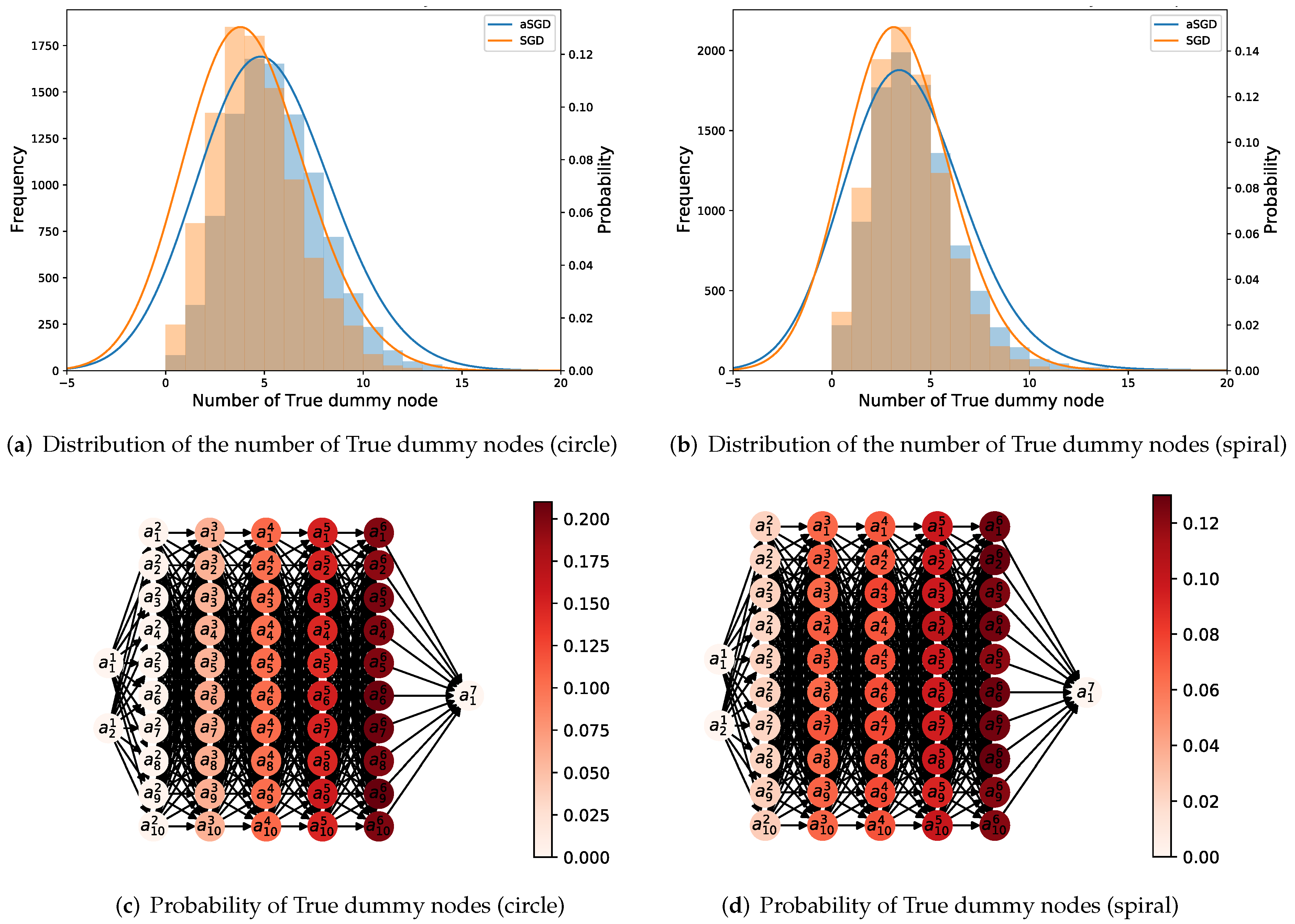
3.1.2. Increasing the Probability of True Dummy Nodes

As shown in Figure 4, in the late stage of training, some parameters ($w_{21}^3$, $w_{22}^3$, $w_{23}^3$, and $b_2^3$) in aSGD are never updated at the later stage of training, while in SGD, this part of the parameters is still updated. It is worth mentioning that we compared the final values of each parameter at the end of training and found that aSGD assigns the gradient of some parameters ($w_{21}^3$, $w_{22}^3$, $w_{23}^3$, and $b_2^3$) to another ($w_{11}^3$, $w_{12}^3$, $w_{13}^3$, and $b_1^3$). This may be the reason for the formation of dummy nodes defined in Section 2. This phenomenon makes the network update parameters selectively. Parameters that are more conducive to reduce loss can be updated, while the others are not updated, which makes redundant nodes become dummy nodes.

3.2. Synthetic Datasets

To further investigate the properties of aSGD and dummy nodes, we use a more redundant network structure and synthetic data for training and testing. We observed the performance of aSGD and SGD on synthetic data. The experiment was repeated 10,000 times and we recorded the step, accuracy, and loss at the end of the training. We counted the location and number of dummy nodes in the network and plotted them into a probability distribution map.

The specific design is as follows: we use a fully connected network to train two kinds of synthetic data, “concentric circles” and “spiral lines”, with SGD and aSGD, respectively. The training samples are shown in Figure 5a. There are four groups of experiments. The training data and test data are sampled in the same pattern of data, and the ratio is 7:3. Groups 1 and 3 use aSGD to train “concentric circle” and “spiral line”, respectively, while Groups 2 and 4 use SGD. The fully connected network is designed with five hidden layers, each with 10 nodes. Except for the activation function of the output node, which is sigmoid, other nodes are ReLU. Parameters are randomly initialized before each training, and 10,000 batches are trained. We stop training with minimal loss or 10,000 batches. The learning rate of Groups 1 and 2 is 0.01, and that of Groups 3 and 4 is 0.05. In total, 128 samples were input for training in the four groups, and the experiment was repeated 10,000 times.

We count the final training results of the two optimizers. Figure 5b shows the final convergence steps of the two optimizers in the two datasets. It can be seen that on the concentric circle data, the two optimizers can train the data in 1000 steps. However, if the training data are more complicated (spiral line), aSGD makes the objective function converge faster than SGD, and the difference between the two is about 1500 steps. For the classification results, we compare the accuracy and loss of the training set and the test set when the model converges in Figure 6, and the results show that aSGD has better accuracy and less loss than SGD. However, due to the redundancy of the network and the simplicity of the synthetic data, the difference in model performance is not too much.

In order to verify that aSGD helps the network generate true dummy nodes, we count the frequency and location of true dummy nodes, as shown in Figure 7.

Comparing the two histograms, it can be found in Figure 7a,b that the number of dummy nodes generated by aSGD is higher than SGD in a single training, whether in concentric circles or spiral lines. On concentric circles, the network trained by aSGD has an average of five more dummy nodes compared to SGD, and it is three in the more complex spiral lines. Generally, in a fixed network structure, whether the parameters are redundant or not is affected by the complexity of the data [35]. These two show that aSGD can adaptively identify redundant parameters in the network according to the complexity of the data and transform them into dummy nodes. This helps us to identify redundant nodes and compress the model.

As is shown in Figure 7c,d, the closer to the output layer, the more likely it is to become a true dummy node. True dummy nodes are more likely to appear on simple datasets; its probability of appearing in the output layer is 0.2 in concentric circles and 0.12 in spiral lines. This may be because in the process of forwarding propagation, the classification results are gradually formed, and there is no need to learn more parameters. This results in a more true dummy node. The probability of nodes in the same layer is similar. This may be due to the fact that the number of nodes in each layer of the network is the same.

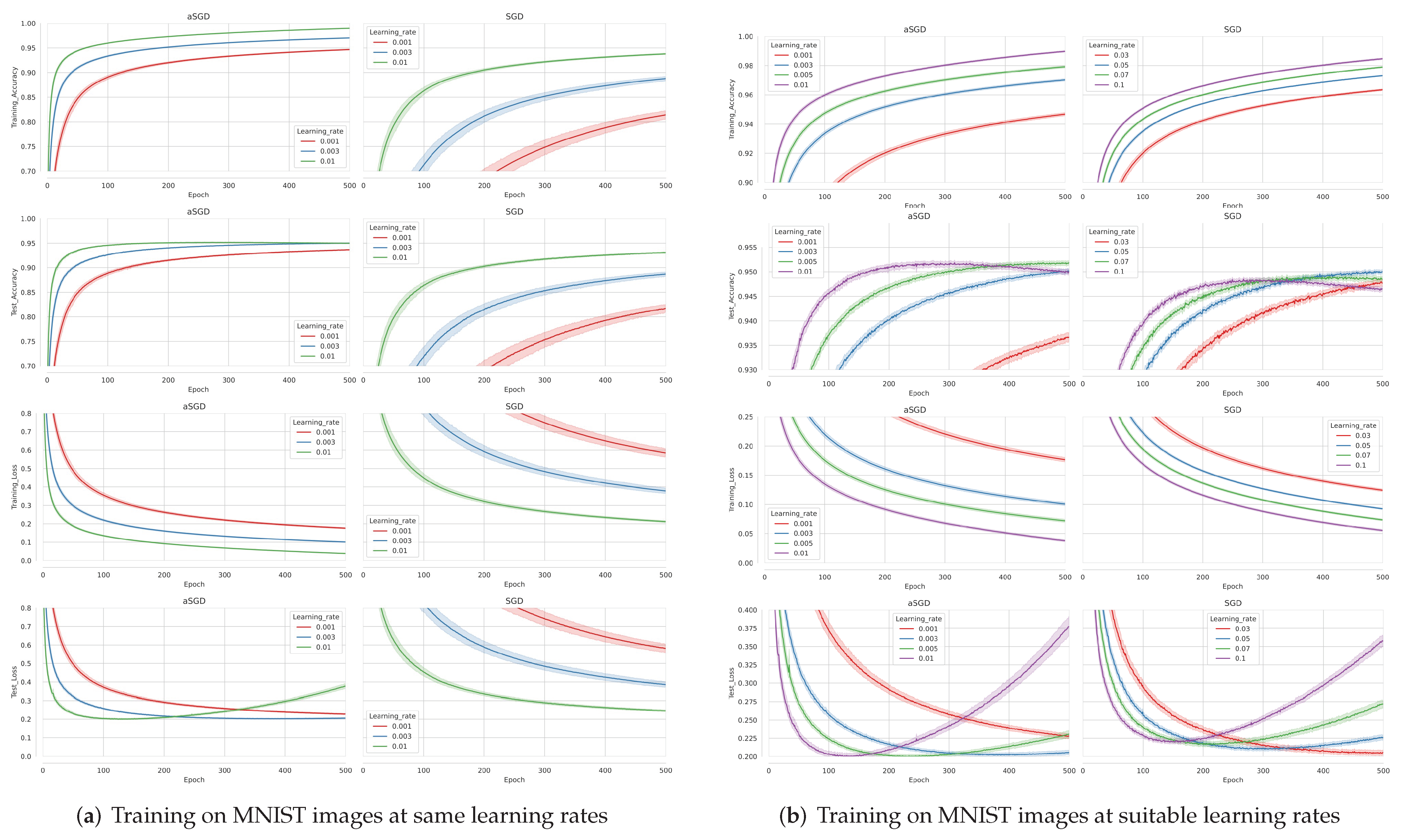
3.3. MNIST Handwritten Digit Dataset

In order to explore the difference between the SGD and aSGD in terms of classification performance, we design the experiment below. The dataset is a MNIST handwritten digit dataset [36]. It contains 60,000 training images and 10,000 test images, and each image is a 28 × 28 gray-scale image. There are 10 classes corresponding to the 10 digits. A fully connected network with two hidden layers is used, and the number of nodes in each layer is 784, 30, 20, and 10. The output layer uses Softmax as the activation function, and the remaining layers still use ReLU. We set the batch size to 64, and train 500 epochs under different learning rates. In this experiment, we do not take early stopping [37] to prevent overfitting. Therefore, we can observe the performance of the two optimizers under different conditions, including underfitting and overfitting. The experiment is repeated 100 times. The learning curves in two cases are presented in Figure 8a,b respectively, one where only the optimizers are different and the hyperparameters are exactly the same, and the other where both optimizers are adjusted to a suitable learning rate.

It can be seen that with the same learning rate, the rates of accuracy increase and loss decrease in aSGD are significantly greater than those of SGD due to a more precisely estimated mean effective gradient. However, increasing the learning rate of SGD can also achieve a similar iteration rate. Therefore, we gradually increase the learning rate within the appropriate range and observe the process of the two optimizers from underfitting to overfitting. It can be found that at the learning rate of 0.01 in Figure 8b, the test loss of aSGD decreases rapidly, and the lowest test loss value that can be achieved is lower than SGD; while SGD cannot achieve both, under the learning rate of 0.03 in Figure 8b, SGD converges to a good test loss value, but the training time is too long. At the learning rate of 0.1 in SGD, the test loss decreases rapidly but cannot achieve a good loss value. In terms of accuracy, aSGD performs better in both training and testing. Comparing the performance of the two optimizers, aSGD has two advantages over SGD: accelerating the training process and achieving higher accuracy. However, the buffer of the learning curve in aSGD is much larger than that of SGD. At the learning rate of 0.01 in aSGD, the buffer of the test loss curve becomes larger in the late training stages. This may be because the adaptive batch is always less than or equal to the hyperparameter batch size, which has the same effect as increasing the learning rate. This means that aSGD is more unstable than SGD, especially in the later stages of training. Therefore, additional methods, such as early stop, learning rate schedules [38], dropout [39], and batch normalization [40], should be added to aSGD.

The mean and standard deviation of the lowest test loss obtained from 100 experiments with the corresponding test accuracy, train accuracy, and train loss are summarized in

Table 1. The mean and variance of the model performance trained on MNIST images at same learning rates.

Method	Learning Rate	Train Accuracy	Train Loss	Test Accuracy	Test Loss
aSGD	0.001	0.9464 ± 0.0055	0.1774 ± 0.0194	0.9372 ± 0.0044	0.2253 ± 0.0172
SGD	0.001	0.8137 ± 0.0438	0.5859 ± 0.1174	0.8186 ± 0.0430	0.5783 ± 0.1189
aSGD	0.003	0.9645 ± 0.0033	0.1189 ± 0.0117	0.9488 ± 0.0027	0.1965 ± 0.0126
SGD	0.003	0.8874 ± 0.0234	0.3787 ± 0.0774	0.8876 ± 0.0231	0.3834 ± 0.0778
aSGD	0.01	0.9652 ± 0.0039	0.1168 ± 0.0135	0.9498 ± 0.0034	0.1922 ± 0.0164
SGD	0.01	0.9376 ± 0.0063	0.2131 ± 0.0252	0.9317 ± 0.0062	0.2423 ± 0.0257

and

Table 2. The mean and variance of the model performance trained on MNIST images at suitable learning rates.

Method	Learning Rate	Train Accuracy	Train Loss	Test Accuracy	Test Loss
	0.001	0.9464 ± 0.0055	0.1774 ± 0.0194	0.9372 ± 0.0044	0.2253 ± 0.0172
aSGD	0.003	0.9645 ± 0.0033	0.1189 ± 0.0117	0.9488 ± 0.0027	0.1965 ± 0.0126
	0.005	0.9652 ± 0.0039	0.1168 ± 0.0135	0.9498 ± 0.0034	0.1922 ± 0.0164
	0.01	0.9662 ± 0.0032	0.1135 ± 0.0102	0.9493 ± 0.0029	0.1937 ± 0.0112
	0.01	0.9376 ± 0.0063	0.2131 ± 0.0252	0.9317 ± 0.0062	0.2423 ± 0.0257
	0.03	0.9615 ± 0.0036	0.1311 ± 0.0129	0.9484 ± 0.0034	0.1984 ± 0.0176
SGD	0.05	0.9625 ± 0.0033	0.1276 ± 0.0111	0.9484 ± 0.0026	0.2023 ± 0.0141
	0.07	0.9611 ± 0.0043	0.1326 ± 0.0145	0.9474 ± 0.0036	0.2074 ± 0.0164
	0.1	0.9599 ± 0.0039	0.1374 ± 0.0137	0.9465 ± 0.0029	0.2099 ± 0.0126

. Trained with the same hyperparameters, aSGD outperforms SGD in both training and testing as shown in Table 1. In Table 2, the learning rates of the two optimizers are adjusted to their appropriate ranges. aSGD achieves the lowest test loss at a learning rate of 0.005, while SGD is 0.03. The best scores are in bold. The loss of aSGD is slightly lower than that of SGD, but it is worth mentioning that aSGD reaches the minimum loss at 100 epochs, while SGD is at 500 epochs, as shown in Figure 8b.

4. Conclusions

In this paper, we analyzed the role of samples in the parameter update by visualizing the process of error backpropagation. Sparse data and features with different frequencies can result in SGD having biased estimates of the expected gradient over the overall training set. With the property of activation function ReLU, we amplified the biased estimation. Based on that, a new adaptive optimization method was proposed from the perspective of the samples, aSGD. An adaptive batch size was applied to aSGD, which allowed aSGD to estimate the expected gradient over the overall training set more accurately than SGD. This helped to perform gradient descent algorithms efficiently. aSGD performed well on both the synthetic datasets and MNIST handwritten digit dataset. In addition, aSGD helped to transform redundant parameters into true dummy nodes, which is beneficial for finding redundant nodes and compress models. However, the current aSGD is a simple method. It can be unstable in the later stages of training and needs to be used with other optimization methods. The difference in parameter updates due to samples can only be amplified by the ReLU function currently. Therefore, aSGD can only be applied to neural networks with ReLU functions. However, many activation functions are common in deep learning, such as sigmoid, tanH, and step function. Distinguishing the differences in parameter updates due to samples under those activation functions and developing new adaptive parameter updating methods need further study.

References

1. Ciregan, D.; Meier, U.; Schmidhuber, J. Multi-column deep neural networks for image classification. In Proceedings of the 2012 IEEE Conference on Computer Vision and Pattern Recognition, Providence, RI, USA, 16–21 June 2012; IEEE: Manhattan, New York, NY, USA, 2012; pp. 3642–3649. [Google Scholar]
2. Dahl, G.E.; Yu, D.; Deng, L.; Acero, A. Context-dependent pre-trained deep neural networks for large-vocabulary speech recognition. IEEE Trans. Audio Speech Lang. Process. 2011, 20, 30–42. [Google Scholar] [CrossRef] [Green Version]
3. Fakoor, R.; Ladhak, F.; Nazi, A.; Huber, M. Using deep learning to enhance cancer diagnosis and classification. In Proceedings of the International Conference on Machine Learning; ACM: New York, NY, USA, 2013; Volume 28, pp. 3937–3949. [Google Scholar]
4. Munir, K.; Elahi, H.; Ayub, A.; Frezza, F.; Rizzi, A. Cancer diagnosis using deep learning: A bibliographic review. Cancers 2019, 11, 1235. [Google Scholar] [CrossRef] [PubMed] [Green Version]
5. Devi, S.R.; Arulmozhivarman, P.; Venkatesh, C.; Agarwal, P. Performance comparison of artificial neural network models for daily rainfall prediction. Int. J. Autom. Comput. 2016, 13, 417–427. [Google Scholar] [CrossRef]
6. Hashim, F.; Daud, N.N.; Ahmad, K.; Adnan, J.; Rizman, Z. Prediction of rainfall based on weather parameter using artificial neural network. J. Fundam. Appl. Sci. 2017, 9, 493–502. [Google Scholar] [CrossRef] [Green Version]
7. Chattopadhyay, S.; Chattopadhyay, G. Conjugate gradient descent learned ANN for Indian summer monsoon rainfall and efficiency assessment through Shannon-Fano coding. J. Atmos. Sol.-Terr. Phys. 2018, 179, 202–205. [Google Scholar] [CrossRef]
8. Bojarski, M.; Del Testa, D.; Dworakowski, D.; Firner, B.; Flepp, B.; Goyal, P.; Jackel, L.D.; Monfort, M.; Muller, U.; Zhang, J.; et al. End to end learning for self-driving cars. arXiv 2016, arXiv:1604.07316. [Google Scholar]
9. Rao, Q.; Frtunikj, J. Deep learning for self-driving cars: Chances and challenges. In Proceedings of the 1st International Workshop on Software Engineering for AI in Autonomous Systems, Gothenburg, Sweden, 28 May 2018; pp. 35–38. [Google Scholar]
10. Han, J.; Moraga, C. The influence of the sigmoid function parameters on the speed of backpropagation learning. In International Workshop on Artificial Neural Networks; Springer: Berlin/Heidelberg, Germany, 1995; pp. 195–201. [Google Scholar]
11. Agarap, A.F. Deep learning using rectified linear units (relu). arXiv 2018, arXiv:1803.08375. [Google Scholar]
12. Nwankpa, C.; Ijomah, W.; Gachagan, A.; Marshall, S. Activation functions: Comparison of trends in practice and research for deep learning. arXiv 2018, arXiv:1811.03378. [Google Scholar]
13. Rumelhart, D.E.; Hinton, G.E.; Williams, R.J. Learning internal representations by error propagation. In Report, California Univ San Diego La Jolla Inst for Cognitive Science; MIT Press: Cambridge, MA, USA, 1985. [Google Scholar]
14. Geyer, C.J. Markov Chain Monte Carlo Maximum Likelihood; Interface Foundation of North America: Fairfax Sta, VA, USA, 1991. [Google Scholar]
15. Bäck, T.; Schwefel, H.P. An overview of evolutionary algorithms for parameter optimization. Evol. Comput. 1993, 1, 1–23. [Google Scholar] [CrossRef]
16. Sutton, R.S.; Barto, A.G. Reinforcement Learning: An Introduction; MIT Press: Cambridge, MA, USA, 2018. [Google Scholar]
17. Ruder, S. An overview of gradient descent optimization algorithms. arXiv 2016, arXiv:1609.04747. [Google Scholar]
18. Dauphin, Y.; Pascanu, R.; Gulcehre, C.; Cho, K.; Ganguli, S.; Bengio, Y. Identifying and attacking the saddle point problem in high-dimensional non-convex optimization. arXiv 2014, arXiv:1406.2572. [Google Scholar]
19. Sutskever, I.; Martens, J.; Dahl, G.; Hinton, G. On the importance of initialization and momentum in deep learning. In International Conference on Machine Learning; PMLR: Atlanta, GA, USA, 2013; pp. 1139–1147. [Google Scholar]
20. Duchi, J.; Hazan, E.; Singer, Y. Adaptive subgradient methods for online learning and stochastic optimization. J. Mach. Learn. Res. 2011, 12, 2121–2159. [Google Scholar]
21. Zeiler, M.D. Adadelta: An adaptive learning rate method. arXiv 2012, arXiv:1212.5701. [Google Scholar]
22. Tieleman, T.; Hinton, G. Lecture 6.5-rmsprop: Divide the gradient by a running average of its recent magnitude. Coursera Neural Netw. Mach. Learn. 2012, 4, 26–31. [Google Scholar]
23. Kingma, D.; Ba, J. Adam: A Method for Stochastic Optimization. arXiv 2014, arXiv:1412.6980. [Google Scholar]
24. Bergstra, J.S.; Bardenet, R.; Bengio, Y.; Kégl, B. Algorithms for hyper-parameter optimization. In Advances in Neural Information Processing Systems; Morgan Kaufmann Publishers Inc.: San Francisco, CA, USA, 2011; pp. 2546–2554. [Google Scholar]
25. Smith, S.L.; Kindermans, P.J.; Ying, C.; Le, Q.V. Don’t decay the learning rate, increase the batch size. arXiv 2017, arXiv:1711.00489. [Google Scholar]
26. Radiuk, P.M. Impact of training set batch size on the performance of convolutional neural networks for diverse datasets. Inf. Technol. Manag. Sci. 2017, 20, 20–24. [Google Scholar] [CrossRef]
27. Bengio, Y.; Senécal, J.S. Quick Training of Probabilistic Neural Nets by Importance Sampling; AISTATS: Key West, FL, USA, 2003; pp. 1–9. [Google Scholar]
28. Zhao, P.; Zhang, T. Accelerating minibatch stochastic gradient descent using stratified sampling. arXiv 2014, arXiv:1405.3080. [Google Scholar]
29. Yang, N.; Tang, H.; Yue, J.; Yang, X.; Xu, Z. Accelerating the Training Process of Convolutional Neural Networks for Image Classification by Dropping Training Samples Out. IEEE Access 2020, 8, 142393–142403. [Google Scholar] [CrossRef]
30. Glorot, X.; Bengio, Y. Understanding the difficulty of training deep feedforward neural networks. In Proceedings of the Thirteenth International Conference on Artificial Intelligence and Statistics, Sardinia, Italy, 3–15 May 2010; pp. 249–256. [Google Scholar]
31. Canziani, A.; Paszke, A.; Culurciello, E. An analysis of deep neural network models for practical applications. arXiv 2016, arXiv:1605.07678. [Google Scholar]
32. Nair, V.; Hinton, G.E. Rectified Linear Units Improve Restricted Boltzmann Machines; ICML: Haifa, Israel, 2010. [Google Scholar]
33. Goodfellow, I.; Bengio, Y.; Courville, A.; Bengio, Y. Deep Learning; MIT Press: Cambridge, UK, 2016; Volume 1. [Google Scholar]
34. Ji Chao, T.H. Visualization and Coding of Original Feature Space Partitioning Process Based on Fully Connected Neural Network. J. Signal Process. 2020, 36, 486–494. [Google Scholar] [CrossRef]
35. Goodfellow, I.; Bengio, Y.; Courville, A. Machine learning basics. Deep Learn. 2016, 1, 98–164. [Google Scholar]
36. LeCun, Y.; Bottou, L.; Bengio, Y.; Haffner, P. Gradient-based learning applied to document recognition. Proc. IEEE 1998, 86, 2278–2324. [Google Scholar] [CrossRef] [Green Version]
37. Yao, Y.; Rosasco, L.; Caponnetto, A. On early stopping in gradient descent learning. Constr. Approx. 2007, 26, 289–315. [Google Scholar] [CrossRef]
38. Robbins, H.; Monro, S. A stochastic approximation method. Ann. Math. Stat. 1951, 22, 400–407. [Google Scholar] [CrossRef]
39. Srivastava, N.; Hinton, G.; Krizhevsky, A.; Sutskever, I.; Salakhutdinov, R. Dropout: A simple way to prevent neural networks from overfitting. J. Mach. Learn. Res. 2014, 15, 1929–1958. [Google Scholar]
40. Ioffe, S.; Szegedy, C. Batch normalization: Accelerating deep network training by reducing internal covariate shift. arXiv 2015, arXiv:1502.03167. [Google Scholar]
Figure 1. (a) “Concentric Circle” dataset and (b) network structure.
Mathematics 10 00863 g001
Figure 2. Backpropagation Equation (2): the visualized factors are listed below each sub-graph. Each point means a sample, and the color represents their value. Red dots are positive, blue dots are negative, and gray dots are 0. It can be seen intuitively that because some points of ReLU ( z 1 3 ) are 0, part of δ 1 3 becomes 0 through the Hadamard product. Some “errors” in δ 1 4 cannot propagate to δ 1 3 . In addition, node a 2 3 is the true dummy node. It completely hinders δ 1 4 propagating to δ 2 3 .
Mathematics 10 00863 g002
Figure 3. Backpropagation Equations (3) and (4). the visualized factors are listed below each sub-graph. Each point means a sample, and the color represents their value. Red dots are positive, blue dots are negative, and gray dots are 0. It can be seen intuitively that because some points of δ 1 3 are 0, part of C / b 1 3 becomes 0. Due to the different contributions of multiple samples to the same parameter update, SGD has biases in the expectation estimation of C / b 1 3 . Some points of a 1 3 that are 0 lead to part of C / w 11 4 becoming 0. Even if the “error” is not 0, there are also biases in this estimation. In addition, node a 2 3 is the true dummy node. Because the “error” δ 1 3 and activation a 1 3 of all samples are 0, the parameters C / b 2 3 and C / w 1 2 4 are no longer updated.
Mathematics 10 00863 g003
Figure 4. The values of each parameter of the model for Experiment 1 during training process with (a) aSGD and (b) SGD. Each subfigure represents the parameters in a layer of the network. The horizontal coordinate is the number of iterations, and the vertical coordinate is the value of the parameter. Each line represents a parameter, including weights and bias. The same parameter is the same color in (a) aSGD and (b) SGD.
Mathematics 10 00863 g004
Figure 5. (a) Synthetic datasets and (b) the boxplot of final convergence steps of Experiment 2.
Mathematics 10 00863 g005
Figure 6. The boxplots of final (a) train accuracy, (b) test accuracy, (c) train loss and (d) test loss of Experiment 2.
Mathematics 10 00863 g006
Figure 7. Histogram of true dummy nodes of (a) “concentric circles” and (b) “spiral lines”, it means the number of true dummy nodes generated by the network in one training. The probability of true dummy nodes in (c) “concentric circles” and (d) “spiral lines” at different locations of network.
Mathematics 10 00863 g007
Figure 8. The learning curve of Experiment 3 for training on MNIST images at (a) same and (b) suitable learning rates using aSGD and SGD. Lines with buffers show the mean and 95% confidence interval.
Mathematics 10 00863 g008