An Efficient Technique of Fractional-Order Physical Models Involving ρ-Laplace Transform

Abstract

In this article, the $\rho$-Laplace transform is paired with a new iterative method to create a new hybrid methodology known as the new iterative transform method (NITM). This method is applied to analyse fractional-order third-order dispersive partial differential equations. The suggested technique procedure is straightforward and appealing, and it may be used to solve non-linear fractional-order partial differential equations effectively. The Caputo operator is used to express the fractional derivatives. Four numerical problems involving fractional-order third-order dispersive partial differential equations are presented with their analytical solutions. The graphs determined that their findings are in excellent agreement with the precise answers to the targeted issues. The solution to the problems at various fractional orders is achieved and found to be correct while comparing the exact solutions at integer-order problems. Although both problems are the non-linear fractional system of partial differential equations, the present technique provides its solution sophisticatedly. Including both integer and fractional order issues, solution graphs are carefully drawn. The fact that the issues’ physical dynamics completely support the solutions at both fractional and integer orders is significant. Moreover, despite using very few terms of the series solution attained by the present technique, higher accuracy is observed. In light of the various and authentic features, it can be customized to solve different fractional-order non-linear systems in nature.

1. Introduction

Fractional calculus (FC) has been a significant field of applied sciences for a few decades. They model actual phenomena with fractional-order integral and derivative answers better than classical derivatives. In modelling many physical phenomena, certain signification implementation can be traced, especially genetics algorithm, signal processing, visco-elasticity damping, transport schemes, electronics, biology, communication, physics, robotics, finance, and chemistry. In the area of FC, scientists are focusing on many significant contributions and discoveries [1,2,3,4]. Due to its appealing applications, FC is a significant study subject for most scholars, and the analysis of fractional-order partial differential equations (PDEs) has drawn special interest from several areas. As a result, various approaches to solving linear and non-linear fractional PDEs have been developed. The local meshless technique, for example, is used to solve fractional-order and anomalous mobile-immobile result transport producers [5,6,7,8,9].

Recently, fractional-order differential equations (FPDES) have been studied to model various non-linear and complex phenomena in nature. FPDEs make a novel contribution towards various scientific research areas, such as a vast range of systems and processes, memories and other fields of science and engineering. The FPDE mathematical models, either for space or time, are both more accurate and they describe many natural phenomena [10,11,12,13,14]. FPDEs have gained the attention of many mathematicians in the field of control theory, dielectric polarization, anomalous diffusion and other problems in science and engineering [15,16]. To describe the properties related to hereditary and the memory of different processes and materials where the past state influences the future state, FPDEs offers an outstanding tool to explain such types of systems because PDEs of integer order does not work as appropriate as fractional order. FPDEs are used to model various scientific phenomena and problems; biology, chemistry, psychology and acoustics, mathematical physics, coloured noises and continuum mechanics. There are remarkable applications of FPDEs in different branches of physics and hydrology [17,18,19]. The main reason FPDEs have gained popularity is that, by nature, the fractional derivative is global while the derivative of integer order is local [20,21,22,23,24,25].

Researchers have a keen interest in developing analytical and numerical methods for the solutions to FPDEs. It is always difficult to find the numerical and analytical solutions to FPDEs. However, mathematicians have developed various novel techniques to handle the solutions of FPDEs effectively. Some of these methods include the haar wavelet method [26], the homotopy analysis method [27], the Laplace transform method [28], Bernstein polynomial [29], the Adomian decomposition method [30], the Legendre base method [31], the finite difference method [32,33] variational iteration method [34], Elzaki Decomposition method [35], differential transform method [36], and the natural transform decomposition method [37].

FPDEs are implemented in many physical models in different fields of applied sciences, such as mathematical biology, fluid dynamics, chemical kinetics, fluid dynamics, linear optics, and quantum mechanics. In 1895, the Vries and Korteweg-de introduced a non-dimensionalized model identified as the KdV equation. In many fields of science and technology, such as quantum theory and particle physics, this model is used to study dispersive wave phenomena. In KdV equations, there are two significant dispersive terms: third and fifty order. Plasma physics has been described using the KdV equation of order five [38].

Fahd and Abdeljawad recently published a paper on the fractional-order $\rho$-Laplace transform Caputo derivative. To examine fractional-order ODEs and PDEs in the sense of Caputo fractional derivative, we proposed a new iterative approach using $\rho$-Laplace transform. Many fractional-order differential equations, including linear and non-linear fractional-order Zakherov–Kuznetsov equations, diffusion equations and Fokker-Planck equations, are solved using this innovative approach.

2. Basic Definitions

The generalised fractional derivative, generalised fractional integral, Mittag–Lefller function, and $\rho$-Laplace transform are all described in this section.

Definition 1.

A continuous function’s generalised fractional-order integral δ$g:[0,+\infty ]\to R$ is expressed as [39]:

$$\left(I^{\delta ,\rho }g\right)\left(\psi \right)=\frac{1}{\mathsf{\Gamma }\left(\delta \right)}{\int }_0^{\psi }{\left(\frac{{\psi }^{\rho }-s^{\rho }}{\rho }\right)}^{\delta -1}\frac{g\left(s\right)ds}{s^{1-\rho }},\rho >0,\psi >0and0<\delta <1.$$

Definition 2.

The generalised continuous functions of a fractional-order derivative δ$g:[0,+\infty ]\to R$ is given as [39]:

$$\left(D^{\delta ,\rho }g\right)\left(\psi \right)=\left(I^{1-\delta ,\rho }g\right)\left(\psi \right)=\frac{1}{\mathsf{\Gamma }(1-\delta )}\left(\frac{d}{d\psi }\right){\int }_0^{\psi }{\left(\frac{{\psi }^{\rho }-s^{\rho }}{\rho }\right)}^{-\delta }\frac{g\left(s\right)ds}{s^{1-\rho }}.\rho >0,\psi >0and0<\delta <1.$$

Definition 3.

The continuous function of Caputo fractional derivative of δ at $g:[0,+\infty ]\to R$ is defined as [39]:

$$\left(D^{\delta ,\rho }g\right)\left(\psi \right)=\frac{1}{\mathsf{\Gamma }(1-\delta )}\left(\frac{d}{d\psi }\right){\int }_0^{\psi }{\left(\frac{{\psi }^{\rho }-s^{\rho }}{\rho }\right)}^{-\delta }{\gamma }^n\frac{g\left(s\right)ds}{s^{1-\rho }}.$$

where $\rho >0$, $\psi >0$, $\gamma ={\psi }^{1-\gamma }\frac{d}{d\psi }$ and $0<\delta <1$.

Definition 4.

The continuous function of a ρ-Laplace transform $g:[0,+\infty ]\to R$ is defined as [39]:

$$L_{\rho }\left\{g\left(\psi \right)\right\}\left(s\right)={\int }_0^{\infty }{e}^{-s\frac{{\psi }^{\rho }}{\rho }}g\left(\psi \right)\frac{d\psi }{{\psi }^{1-\rho }}.$$

The ρ-Laplace transform Caputo generalized fractional-order derivative of a continuous function g is given as [39]:

$$\begin{array}{c}\hfill L_{\rho }\left\{D^{\delta ,\rho }g\left(\psi \right)\right\}\left(s\right)=s^{\delta }{L}_{\rho }\left\{g\left(\psi \right)\right\}-\sum _{k=0}^{n-1}{s}^{\delta -k-1}\left(I^{\delta ,\rho }{\gamma }^{n}g\right)\left(0\right).\end{array}$$

Definition 5.

The generalized Mittag–Leffler function is define as:

$$E_{\delta ,\rho }\left(z\right)=\sum _{k=0}^{\infty }\frac{z^{\delta }}{\mathsf{\Gamma }(\delta k+\rho )}.$$

3. The General Implementation of Methodology

Consider the functional equation

$$\begin{array}{c}\hfill \phi =g+G\left(\phi \right)+N\left(\phi \right),\end{array}$$

(1)

where g is a source function, G is linear and N non-linear terms, respectively. Let us consider analysis of Equation (1) is given as:

$$\begin{array}{cc}\hfill {\phi }_0& =g,\hfill \\ \hfill {\phi }_1& =G\left({\phi }_0\right)+N\left({\phi }_0\right),\hfill \\ \hfill {\phi }_{m+1}& =G({\phi }_m)+(N(\sum _{\kappa =0}^{\infty }{\phi }_m(r))-N(\sum _{\kappa =0}^{\infty }{\phi }_{\kappa }(r))),\hfill \end{array}$$

(2)

where $m=1,2,3\cdots$,

$$\begin{array}{c}\hfill \phi =\sum _{\kappa =0}^{\infty }{\phi }_{\kappa }.\end{array}$$

(3)

Now, linear and non-linear terms can be expressed as [30]:

$$\begin{array}{cc}\hfill G(\phi )& =G(\sum _{\kappa =0}^{\infty }{\phi }_{\kappa })=(\sum _{\kappa =0}^{\infty }G({\phi }_{\kappa })),\hfill \\ \hfill N(\phi )=N(\sum _{\kappa =0}^{\infty }{\phi }_{\kappa })& =N({\phi }_0)+\sum _{\kappa =1}^{\infty }\{N(\sum _{j=0}^{\kappa }{\phi }_j)-N(\sum _{j=0}^{\kappa -1}{\phi }_j)\}.\hfill \end{array}$$

(4)

We obtain the solution of (1) as:

$$\begin{array}{c}\hfill \phi =g+\sum _{\kappa =0}^{\infty }G({\phi }_{\kappa })+N({\phi }_0)+\sum _{\kappa =1}^{\infty }\{N(\sum _{j=0}^{\kappa }{\phi }_j)-N(\sum _{j=0}^{\kappa -1}{\phi }_j)\}.\end{array}$$

(5)

Consider the fractional-order Caputo derivative equation is given as:

$$\begin{array}{c}\hfill D^{\delta ,\rho }\phi (\epsilon ,\eta )+N\phi (\epsilon ,\eta )=g(\epsilon ,\eta ),\end{array}$$

(6)

the initial condition $\phi (\epsilon ,0)=g\left(\epsilon \right)$, where N is a non-linear term.

Now applying $\rho$-Laplace transform of Equation (6), we get:

$$\begin{array}{c}\hfill L_{\rho }(D^{\delta ,\rho }\phi (\epsilon ,\eta )+Nu(\epsilon ,\eta ))=L_{\rho }\left(g(\epsilon ,\eta )\right);\end{array}$$

(7)

applying $\rho$-Laplace transform, we achieve:

$$\begin{array}{c}\hfill s^{\delta }\phi (\epsilon ,\eta )-s^{\delta -1}\phi (\epsilon ,0)=L_{\rho }\left(g(\epsilon ,\eta )\right)-L_{\rho }\left(N\phi (\epsilon ,\eta )\right).\end{array}$$

(8)

Simplify (8), we get:

$$\begin{array}{c}\hfill \phi (\epsilon ,\eta )=\frac{{\phi }_0(\epsilon ,0)}{s}+s^{-\delta }{L}_{\rho }\left(g(\epsilon ,\eta )\right)-s^{-\delta }{L}_{\rho }\left(N\phi (\epsilon ,\eta )\right).\end{array}$$

(9)

Using inverse Laplace transform of (10), we have:

$$\begin{array}{c}\hfill \phi (\epsilon ,\eta )={\phi }_0(\epsilon ,0)+L_{\rho }^{-1}\left(s^{-\delta }{L}_{\rho }\left(g(\epsilon ,\eta )\right)\right)-L_{\rho }^{-1}\left(s^{-\delta }{L}_{\rho }\left(Nu(\epsilon ,\eta )\right)\right).\end{array}$$

(10)

Applying new iterative method, we get

$$\begin{array}{cc}\hfill g& =\phi (\epsilon ,0),\hfill \\ \hfill L\left(\phi \right)& =L_{\rho }^{-1}\left(s^{-\delta }{L}_{\rho }\left(g(\epsilon ,\eta )\right)\right),\hfill \\ \hfill N\left(\phi \right)& =-L_{\rho }^{-1}\left(s^{-\delta }{L}_{\rho }\left(N\phi (\epsilon ,\eta )\right)\right).\hfill \end{array}$$

(11)

The recurrence relation is defined as:

$$\begin{array}{cc}\hfill {\phi }_0& =g,\hfill \\ \hfill {\phi }_1& =L({\phi }_0)+N({\phi }_0),\hfill \\ \hfill {\phi }_{m+1}& =L({\phi }_m)+(N(\sum _{\kappa =0}^{\infty }{\phi }_m(r))-N(\sum _{\kappa =0}^{m-1}{\phi }_{\kappa }(r))),\hfill \end{array}$$

(12)

where $m=1,2,3\cdots$, Hence, the solution of Equation (6) is define as,

$$\begin{array}{c}\hfill \sum _{\kappa =0}^{\infty }{\phi }_{\kappa }=g+L(\sum _{\kappa =0}^{\infty }{\phi }_{\kappa })+N(\sum _{\kappa =0}^{\infty }{\phi }_{\kappa }).\end{array}$$

(13)

4. Convergence of NITM

Now, we discus the condition for convergence of NITM.

Theorem 1.

If N is $C^{(\infty )}$ in a neighborhood of $u_0$ and [40]

$$∥N^{\left(n\right)}\left(u_0\right)∥=Sup\left\{N^{\left(n\right)}\left(u_0\right)\left(h_1,\dots ,h_n\right):∥h_i∥\le 1,1\le i\le n\right\}\le L$$

for any n and for some real $L>0$ and $∥u_i∥\le M<1/e,i=1,2,\dots$, then the series ${\sum }_{n=0}^{\infty }{G}_n$ is absolutely convergent, and moreover,

$$∥G_n∥\le L{M}^n{e}^{n-1}(e-1),n=1,2,\dots$$

Proof. 

In view of (13),

$$∥G_n∥\le L{M}^n\sum _{i_n=1}^{\infty }\sum _{n-1}^{\infty }\cdots \sum _{i_1=0}^{\infty }\left(\prod _{j=1}^n\frac{1}{i_j!}\right)=L{M}^n{e}^{n-1}(e-1).$$

Thus, the series ${\sum }_{n=1}^{\infty }∥G_n∥$ is dominated by the convergent series $LM(e-1){\sum }_{n=1}^{\infty }$${\left(Me\right)}^{n-1}$, where $M<1/e$. Hence, ${\sum }_{n=0}^{\infty }{G}_n$ is absolutely convergent, due to the comparison test. □

As it is difficult to show bounded ness of $∥u_i∥$, for all i, a more useful result is proved in the following theorem, where conditions on $N^{\left(k\right)}\left(u_0\right)$ are given which are sufficient to guarantee convergence of the series.

Theorem 2.

If N is $C^{(\infty )}$ and $∥N^{\left(n\right)}\left(u_0\right)∥\le M\le e^{-1}$, for all n, then the series ${\sum }_{n=0}^{\infty }{G}_n$ is absolutely convergent [40].

Proof. 

Consider the recurrence relation

$${\xi }_n={\xi }_{0}exp\left({\xi }_{n-1}\right),n=1,2,3,\dots ,$$

where ${\xi }_0=M$. Define ${\eta }_n={\xi }_n-{\xi }_{n-1},n=1,2,3,\dots$ Using (13), (11), and the hypothesis of Theorem 2, we observe that

$$∥G_n∥\le {\eta }_n,n=1,2,3,\cdots$$

Let

$${\sigma }_n=\sum _{i=1}^n{\eta }_i={\xi }_n-{\xi }_0.$$

Note that ${\xi }_0=e^{-1}>0,{\xi }_1={\xi }_{0}exp\left({\xi }_0\right)>{\xi }_0$, and ${\xi }_2={\xi }_{0}exp\left({\xi }_1\right)>{\xi }_{0}exp\left({\xi }_0\right)={\xi }_1$. In general, ${\xi }_n>{\xi }_{n-1}>0$. Hence, $\sum {\eta }_n$ is a series of positive real numbers. Note that:

$$\begin{array}{c}0<{\xi }_0=M=e^{-1}<1\\ 0<{\xi }_1={\xi }_{0}exp\left({\xi }_0\right)<{\xi }_0{e}^1=e^{-1}{e}^1=1\\ 0<{\xi }_2={\xi }_{0}exp\left({\xi }_1\right)<{\xi }_0{e}^1=1\end{array}$$

In general, $0<{\xi }_n<1$. Hence, ${\sigma }_n={\xi }_n-{\xi }_0<1$. This implies that ${\left\{{\sigma }_n\right\}}_{n=1}^{\infty }$ is bounded above by 1 , and hence convergent. Therefore, $\sum G_n$ is absolutely convergent by the comparison test. □

5. Application to Kdv Equations

Example 1.

Consider the fractional dispersive KdV equation is given as [41]:

$$\begin{array}{c}\hfill D_{\eta }^{\delta ,\rho }\phi (\epsilon ,\eta )+2\frac{\partial \phi (\epsilon ,\eta )}{\partial \epsilon }+\frac{{\partial }^3\phi (\epsilon ,\eta )}{\partial {\epsilon }^3}=0,\eta >0,0<\delta \le 1,\end{array}$$

(14)

with $\phi (x,0)=sin\epsilon$. Applying ρ-Laplace transform of Equation (14), we have:

$$\begin{array}{c}\hfill \phi (\epsilon ,s)=\frac{L_{\rho }\left({\phi }_{\eta }\right)+s^{\delta -1}\phi (\epsilon ,0)}{s^{\delta }},\end{array}$$

(15)

from which,

$$\begin{array}{c}\hfill \phi (\epsilon ,\eta )=\frac{sin\epsilon }{s}-\frac{L_{\rho }\left\{2\frac{\partial \phi (\epsilon ,\eta )}{\partial \epsilon }+\frac{{\partial }^3\phi (\epsilon ,\eta )}{\partial {\epsilon }^3}\right\}}{s^{\delta }}.\end{array}$$

(16)

Using inverse ρ-Laplace transform of Equation (16), we get:

$$\begin{array}{c}\hfill \phi (\epsilon ,\eta )=sin\epsilon -L_{\rho }^{-1}\left[\frac{L_{\rho }\left\{2\frac{\partial \phi (\epsilon ,\eta )}{\partial \epsilon }+\frac{{\partial }^3\phi (\epsilon ,\eta )}{\partial {\epsilon }^3}\right\}}{s^{\delta }}\right].\end{array}$$

(17)

Implementing the proposed technique, we get:

$$\begin{array}{cc}\hfill f& ={\phi }_0=sin\epsilon ,\hfill \\ \hfill {\phi }_1(\epsilon ,\eta )& =-L_{\rho }^{-1}\left[\frac{L_{\rho }\left\{2\frac{\partial {\phi }_0(\epsilon ,\eta )}{\partial \epsilon }+\frac{{\partial }^3{\phi }_0(\epsilon ,\eta )}{\partial {\epsilon }^3}\right\}}{s^{\delta }}\right]=-\frac{cos\epsilon }{\mathsf{\Gamma }(1+\delta )}{\left(\frac{{\eta }^{\rho }}{\rho }\right)}^{\delta },\hfill \\ \hfill {\phi }_2(\epsilon ,\eta )& =-L_{\rho }^{-1}\left[\frac{L_{\rho }\left\{2\frac{\partial {\phi }_1(\epsilon ,\eta )}{\partial \epsilon }+\frac{{\partial }^3{\phi }_1(\epsilon ,\eta )}{\partial {\epsilon }^3}\right\}}{s^{\delta }}\right]=-\frac{sin\epsilon }{\mathsf{\Gamma }(1+2\delta )}{\left(\frac{{\eta }^{\rho }}{\rho }\right)}^{2\delta },\hfill \\ \hfill {\phi }_3(\epsilon ,\eta )& =-L_{\rho }^{-1}\left[\frac{L_{\rho }\left\{2\frac{\partial {\phi }_2(\epsilon ,\eta )}{\partial \epsilon }+\frac{{\partial }^3{\phi }_2(\epsilon ,\eta )}{\partial {\epsilon }^3}\right\}}{s^{\delta }}\right]=\frac{cos\epsilon }{\mathsf{\Gamma }(1+3\delta )}{\left(\frac{{\eta }^{\rho }}{\rho }\right)}^{3\delta },\hfill \\ \hfill & ⋮.\hfill \end{array}$$

(18)

Hence, the approximate solution of series form of Equation (14) is given as:

$$\begin{array}{cc}\hfill \phi (\epsilon ,\eta )& ={\phi }_0(\epsilon ,\eta )+{\phi }_1(\epsilon ,\eta )+{\phi }_2(\epsilon ,\eta )+{\phi }_3(\epsilon ,\eta )+\cdots .\hfill \\ \hfill \phi (\epsilon ,\eta )& =sin\epsilon -\frac{cos\epsilon }{\mathsf{\Gamma }(1+\delta )}{\left(\frac{{\eta }^{\rho }}{\rho }\right)}^{\delta }-\frac{sin\epsilon }{\mathsf{\Gamma }(1+2\delta )}{\left(\frac{{\eta }^{\rho }}{\rho }\right)}^{2\delta }+\frac{cos\epsilon }{\mathsf{\Gamma }(1+3\delta )}{\left(\frac{{\eta }^{\rho }}{\rho }\right)}^{3\delta }+\cdots .\hfill \end{array}$$

(19)

The series form solution is given by:

$$\begin{array}{cc}\hfill & \phi (\epsilon ,\eta )=sin\epsilon \left(1-\frac{{\left(\frac{{\eta }^{\rho }}{\rho }\right)}^{2\delta }}{\mathsf{\Gamma }(1+2\delta )}+\frac{{\left(\frac{{\eta }^{\rho }}{\rho }\right)}^{4\delta }}{\mathsf{\Gamma }(1+4\delta )}-\dots \right)\hfill \\ \hfill & -cos\epsilon \left(\frac{{\left(\frac{{\eta }^{\rho }}{\rho }\right)}^{\delta }}{\mathsf{\Gamma }(1+\delta )}-\frac{{\left(\frac{{\eta }^{\rho }}{\rho }\right)}^{3\delta }}{\mathsf{\Gamma }(1+3\delta )}+\frac{{\left(\frac{{\eta }^{\rho }}{\rho }\right)}^{5\delta }}{\mathsf{\Gamma }(1+5\delta )}-\dots \right),\hfill \end{array}$$

(20)

when $\delta =1$, then NITM solution is:

$$\begin{array}{c}\hfill \phi (\epsilon ,\eta )=sin(\epsilon -\eta ).\end{array}$$

(21)

Example 2.

Consider the following fractional dispersive KdV equation is given as [41]:

$$\begin{array}{c}\hfill D_{\eta }^{\delta ,\rho }\phi (\epsilon ,\xi ,\eta )+\frac{{\partial }^3\phi (\epsilon ,\xi ,\eta )}{\partial {\epsilon }^3}+\frac{{\partial }^3\phi (\epsilon ,\xi ,\eta )}{\partial {\xi }^3}=0,\eta >0,0<\delta \le 1,\end{array}$$

(22)

with $\phi (\epsilon ,\xi ,0)=cos(\epsilon +\xi )$. Applying ρ-Laplace transform of Equation (22), we get:

$$\begin{array}{c}\hfill \phi (\epsilon ,\xi ,s)=\frac{L_{\rho }\left({\phi }_{\eta }\right)+s^{\delta -1}\phi (\epsilon ,\xi ,0)}{s^{\delta }},\end{array}$$

(23)

from which,

$$\begin{array}{c}\hfill \phi (\epsilon ,\xi ,\eta )=\frac{cos(\epsilon +\xi )}{s}-\frac{L_{\rho }\left\{\frac{{\partial }^3\phi (\epsilon ,\xi ,\eta )}{\partial {\epsilon }^3}+\frac{{\partial }^3\phi (\epsilon ,\xi ,\eta )}{\partial {\xi }^3}\right\}}{s^{\delta }}.\end{array}$$

(24)

Applying inverse ρ-Laplace transform of (24), we have:

$$\begin{array}{c}\hfill \phi (\epsilon ,\xi ,\eta )=cos(\epsilon +\xi )-L_{\rho }^{-1}\left[\frac{L_{\rho }\left\{\frac{{\partial }^3\phi (\epsilon ,\xi ,\eta )}{\partial {\epsilon }^3}+\frac{{\partial }^3\phi (\epsilon ,\xi ,\eta )}{\partial {\xi }^3}\right\}}{s^{\delta }}\right].\end{array}$$

(25)

Using the proposed technique, we get:

$$\begin{array}{cc}\hfill f& ={\phi }_0(\epsilon ,\xi ,\eta )=cos(\epsilon +\xi ),\hfill \\ \hfill {\phi }_1(\epsilon ,\xi ,\eta )& =-L_{\rho }^{-1}\left[\frac{L_{\rho }\left\{\frac{{\partial }^3{\phi }_0(\epsilon ,\xi ,\eta )}{\partial {\epsilon }^3}+\frac{{\partial }^3{\phi }_0(\epsilon ,\xi ,\eta )}{\partial {\xi }^3}\right\}}{s^{\delta }}\right]=-\frac{2sin(\epsilon +\xi )}{\mathsf{\Gamma }(1+\delta )}{\left(\frac{{\eta }^{\rho }}{\rho }\right)}^{\delta },\hfill \\ \hfill {\phi }_2(\epsilon ,\xi ,\eta )& =-L_{\rho }^{-1}\left[\frac{L_{\rho }\left\{\frac{{\partial }^3{\phi }_1(\epsilon ,\xi ,\eta )}{\partial {\epsilon }^3}+\frac{{\partial }^3{\phi }_1(\epsilon ,\xi ,\eta )}{\partial {\xi }^3}\right\}}{s^{\delta }}\right]=-\frac{4cos(\epsilon +\xi )}{\mathsf{\Gamma }(1+2\delta )}{\left(\frac{{\eta }^{\rho }}{\rho }\right)}^{2\delta },\hfill \\ \hfill {\phi }_3(\epsilon ,\xi ,\eta )& =-L_{\rho }^{-1}\left[\frac{L_{\rho }\left\{\frac{{\partial }^3{\phi }_2(\epsilon ,\xi ,\eta )}{\partial {\epsilon }^3}+\frac{{\partial }^3{\phi }_2(\epsilon ,\xi ,\eta )}{\partial {\xi }^3}\right\}}{s^{\delta }}\right]=\frac{8sin(\epsilon +\xi )}{\mathsf{\Gamma }(1+3\delta )}{\left(\frac{{\eta }^{\rho }}{\rho }\right)}^{3\delta }.\hfill \\ \hfill & ⋮\hfill \end{array}$$

(26)

Hence, the approximate solution of series form of Equation (22) is given as:

$$\begin{array}{cc}\hfill \phi (\epsilon ,\xi ,\eta )& ={\phi }_0(\epsilon ,\xi ,\eta )+{\phi }_1(\epsilon ,\xi ,\eta )+{\phi }_2(\epsilon ,\xi ,\eta )+{\phi }_3(\epsilon ,\xi ,\eta )+\cdots .\hfill \\ \hfill \phi (\epsilon ,\eta )& =cos(\epsilon +\xi )-2\frac{sin(\epsilon +\xi )}{\mathsf{\Gamma }(1+\delta )}{\left(\frac{{\eta }^{\rho }}{\rho }\right)}^{\delta }-4\frac{cos(\epsilon +\xi )}{\mathsf{\Gamma }(1+2\delta )}{\left(\frac{{\eta }^{\rho }}{\rho }\right)}^{2\delta }+8\frac{cos(\epsilon +\xi )}{\mathsf{\Gamma }(1+3\delta )}{\left(\frac{{\eta }^{\rho }}{\rho }\right)}^{3\delta }+\cdots .\hfill \end{array}$$

(27)

The series form solution is given by:

$$\begin{array}{cc}\hfill & \phi (\epsilon ,\xi ,\eta )=cos(\epsilon +\xi )\left(1-4\frac{{\left(\frac{{\eta }^{\rho }}{\rho }\right)}^{2\delta }}{\mathsf{\Gamma }(1+2\delta )}+16\frac{{\left(\frac{{\eta }^{\rho }}{\rho }\right)}^{2\delta }}{\mathsf{\Gamma }(1+2\delta )}-\dots \right)\hfill \\ \hfill & -sin(\epsilon +\xi )\left(\frac{{\left(\frac{{\eta }^{\rho }}{\rho }\right)}^{\delta }}{\mathsf{\Gamma }(1+\delta )}-8\frac{{\left(\frac{{\eta }^{\rho }}{\rho }\right)}^{3\delta }}{\mathsf{\Gamma }(1+3\delta )}+32\frac{{\left(\frac{{\eta }^{\rho }}{\rho }\right)}^{5\delta }}{\mathsf{\Gamma }(1+5\delta )}-\dots \right),\hfill \end{array}$$

(28)

when $\delta =1$, then NITM solution is:

$$\begin{array}{c}\hfill \phi (\epsilon ,\xi ,\eta )=cos(\epsilon +\xi +2\eta ).\end{array}$$

(29)

Example 3.

Consider the fractional dispersive KdV equation is given as [41]:

$$\begin{array}{c}\hfill D_{\eta }^{\delta ,\rho }\phi (\epsilon ,\eta )+\frac{{\partial }^3\phi (\epsilon ,\eta )}{\partial {\xi }^3}=-sin\pi \epsilon sin\eta -{\pi }^{3}cos\pi \epsilon cos\eta ,\eta >0,0<\delta \le 1,\end{array}$$

(30)

with $\phi (\epsilon ,0)=sin\pi \epsilon$. Applying ρ-Laplace transform of Equation (30), we have:

$$\begin{array}{c}\hfill \phi (\epsilon ,s)=\frac{L_{\rho }\left({\phi }_{\eta }\right)+s^{\delta -1}\phi (\epsilon ,0)}{s^{\delta }},\end{array}$$

(31)

from which,

$$\begin{array}{c}\hfill \phi (\epsilon ,\eta )=\frac{sin\pi \epsilon }{s}+\frac{sin\pi \epsilon sin\eta +{\pi }^{3}cos\pi \epsilon cos\eta }{s^{\delta }}-\frac{L_{\rho }\left\{\frac{{\partial }^3\phi (\epsilon ,\eta )}{\partial {\xi }^3}\right\}}{s^{\delta }}.\end{array}$$

(32)

Using inverse ρ-Laplace transform of (32), we get:

$$\begin{array}{cc}\hfill \phi (\epsilon ,\eta )=& sin\pi \epsilon -sin\pi \epsilon \left(\frac{{\left(\frac{{\eta }^{\rho }}{\rho }\right)}^{2\delta }}{\mathsf{\Gamma }(1+2\delta )}-\frac{{\left(\frac{{\eta }^{\rho }}{\rho }\right)}^{4\delta }}{\mathsf{\Gamma }(1+4\delta )}+\frac{{\left(\frac{{\eta }^{\rho }}{\rho }\right)}^{6\delta }}{\mathsf{\Gamma }(1+6\delta )}-\frac{{\left(\frac{{\eta }^{\rho }}{\rho }\right)}^{8\delta }}{\mathsf{\Gamma }(1+8\delta )}+\frac{{\left(\frac{{\eta }^{\rho }}{\rho }\right)}^{10\delta }}{\mathsf{\Gamma }(1+10\delta )}\right)\hfill \\ \hfill & -{\pi }^{3}cos\pi \epsilon \left(\frac{{\left(\frac{{\eta }^{\rho }}{\rho }\right)}^{\delta }}{\mathsf{\Gamma }(1+\delta )}-\frac{{\left(\frac{{\eta }^{\rho }}{\rho }\right)}^{3\delta }}{\mathsf{\Gamma }(1+3\delta )}+\frac{{\left(\frac{{\eta }^{\rho }}{\rho }\right)}^{5\delta }}{\mathsf{\Gamma }(1+5\delta )}-\frac{{\left(\frac{{\eta }^{\rho }}{\rho }\right)}^{7\delta }}{\mathsf{\Gamma }(1+7\delta )}+\frac{{\left(\frac{{\eta }^{\rho }}{\rho }\right)}^{9\delta }}{\mathsf{\Gamma }(1+9\delta )}\right)-L_{\rho }^{-1}\left[\frac{L_{\rho }\left\{\frac{{\partial }^3\phi (\epsilon ,\eta )}{\partial {\xi }^3}\right\}}{s^{\delta }}\right].\hfill \end{array}$$

(33)

Implementing the proposed technique, we get:

$$\begin{array}{cc}\hfill f& ={\phi }_0=sin\pi \epsilon -sin\pi \epsilon \left(\frac{{\left(\frac{{\eta }^{\rho }}{\rho }\right)}^{2\delta }}{\mathsf{\Gamma }(1+2\delta )}-\frac{{\left(\frac{{\eta }^{\rho }}{\rho }\right)}^{4\delta }}{\mathsf{\Gamma }(1+4\delta )}+\frac{{\left(\frac{{\eta }^{\rho }}{\rho }\right)}^{6\delta }}{\mathsf{\Gamma }(1+6\delta )}-\frac{{\left(\frac{{\eta }^{\rho }}{\rho }\right)}^{8\delta }}{\mathsf{\Gamma }(1+8\delta )}+\frac{{\left(\frac{{\eta }^{\rho }}{\rho }\right)}^{10\delta }}{\mathsf{\Gamma }(1+10\delta )}\right)\hfill \\ \hfill & -{\pi }^{3}cos\pi \epsilon \left(\frac{{\left(\frac{{\eta }^{\rho }}{\rho }\right)}^{\delta }}{\mathsf{\Gamma }(1+\delta )}-\frac{{\left(\frac{{\eta }^{\rho }}{\rho }\right)}^{3\delta }}{\mathsf{\Gamma }(1+3\delta )}+\frac{{\left(\frac{{\eta }^{\rho }}{\rho }\right)}^{5\delta }}{\mathsf{\Gamma }(1+5\delta )}-\frac{{\left(\frac{{\eta }^{\rho }}{\rho }\right)}^{7\delta }}{\mathsf{\Gamma }(1+7\delta )}+\frac{{\left(\frac{{\eta }^{\rho }}{\rho }\right)}^{9\delta }}{\mathsf{\Gamma }(1+9\delta )}\right),\hfill \\ \hfill {\phi }_1(\epsilon ,\eta )& =-L_{\rho }^{-1}\left[\frac{L_{\rho }\left\{\frac{{\partial }^3{\phi }_0(\epsilon ,\eta )}{\partial {\xi }^3}\right\}}{s^{\delta }}\right]={\pi }^{3}cos\pi \epsilon \frac{{\left(\frac{{\eta }^{\rho }}{\rho }\right)}^{\delta }}{\mathsf{\Gamma }(1+\delta )}-{\pi }^{3}cos{\pi }^3\epsilon \left(\frac{{\left(\frac{{\eta }^{\rho }}{\rho }\right)}^{3\delta }}{\mathsf{\Gamma }(1+3\delta )}-\frac{{\left(\frac{{\eta }^{\rho }}{\rho }\right)}^{5\delta }}{\mathsf{\Gamma }(1+5\delta )}+\frac{{\left(\frac{{\eta }^{\rho }}{\rho }\right)}^{7\delta }}{\mathsf{\Gamma }(1+7\delta )}\right.\hfill \\ \hfill & \left.-\frac{{\left(\frac{{\eta }^{\rho }}{\rho }\right)}^{9\delta }}{\mathsf{\Gamma }(1+9\delta )}+\frac{{\left(\frac{{\eta }^{\rho }}{\rho }\right)}^{11\delta }}{\mathsf{\Gamma }(1+11\delta )}\right)-{\pi }^{6}sin\pi \epsilon \left(\frac{{\left(\frac{{\eta }^{\rho }}{\rho }\right)}^{2\delta }}{\mathsf{\Gamma }(1+2\delta )}-\frac{{\left(\frac{{\eta }^{\rho }}{\rho }\right)}^{4\delta }}{\mathsf{\Gamma }(1+4\delta )}+\frac{{\left(\frac{{\eta }^{\rho }}{\rho }\right)}^{6\delta }}{\mathsf{\Gamma }(1+6\delta )}-\frac{{\left(\frac{{\eta }^{\rho }}{\rho }\right)}^{8\delta }}{\mathsf{\Gamma }(1+8\delta )}+\frac{{\left(\frac{{\eta }^{\rho }}{\rho }\right)}^{10\delta }}{\mathsf{\Gamma }(1+10\delta )}\right),\hfill \\ \hfill {\phi }_2(\epsilon ,\eta )& =-L_{\rho }^{-1}\left[\frac{L_{\rho }\left\{\frac{{\partial }^3{\phi }_1(\epsilon ,\eta )}{\partial {\xi }^3}\right\}}{s^{\delta }}\right]=-{\pi }^{6}sin\pi \epsilon \frac{{\left(\frac{{\eta }^{\rho }}{\rho }\right)}^{2\delta }}{\mathsf{\Gamma }(1+2\delta )}+{\pi }^{6}sin{\pi }^3\epsilon \left(\frac{{\left(\frac{{\eta }^{\rho }}{\rho }\right)}^{5\delta }}{\mathsf{\Gamma }(1+4\delta )}-\frac{{\left(\frac{{\eta }^{\rho }}{\rho }\right)}^{6\delta }}{\mathsf{\Gamma }(1+6\delta )}+\frac{{\left(\frac{{\eta }^{\rho }}{\rho }\right)}^{8\delta }}{\mathsf{\Gamma }(1+8\delta )}\right.\hfill \\ \hfill & \left.-\frac{{\left(\frac{{\eta }^{\rho }}{\rho }\right)}^{10\delta }}{\mathsf{\Gamma }(1+10\delta )}+\frac{{\left(\frac{{\eta }^{\rho }}{\rho }\right)}^{12\delta }}{\mathsf{\Gamma }(1+12\delta )}\right)+{\pi }^{9}cos\pi \epsilon \left(\frac{{\left(\frac{{\eta }^{\rho }}{\rho }\right)}^{3\delta }}{\mathsf{\Gamma }(1+3\delta )}-\frac{{\left(\frac{{\eta }^{\rho }}{\rho }\right)}^{5\delta }}{\mathsf{\Gamma }(1+5\delta )}+\frac{{\left(\frac{{\eta }^{\rho }}{\rho }\right)}^{7\delta }}{\mathsf{\Gamma }(1+7\delta )}-\frac{{\left(\frac{{\eta }^{\rho }}{\rho }\right)}^{9\delta }}{\mathsf{\Gamma }(1+9\delta )}+\frac{{\left(\frac{{\eta }^{\rho }}{\rho }\right)}^{11\delta }}{\mathsf{\Gamma }(1+11\delta )}\right).\hfill \\ \hfill & ⋮\hfill \end{array}$$

(34)

Hence, the approximate solution of Equation (30) is given as:

$$\begin{array}{cc}\hfill \phi (\epsilon ,\eta )& ={\phi }_0(\epsilon ,\eta )+{\phi }_1(\epsilon ,\eta )+{\phi }_2(\epsilon ,\eta )+{\phi }_3(\epsilon ,\eta )+\cdots .\hfill \\ \hfill \phi (\epsilon ,\eta )& =sin\pi \epsilon -sin\pi \epsilon \left(\frac{{\left(\frac{{\eta }^{\rho }}{\rho }\right)}^{2\delta }}{\mathsf{\Gamma }(1+2\delta )}-\frac{{\left(\frac{{\eta }^{\rho }}{\rho }\right)}^{4\delta }}{\mathsf{\Gamma }(1+4\delta )}+\frac{{\left(\frac{{\eta }^{\rho }}{\rho }\right)}^{6\delta }}{\mathsf{\Gamma }(1+6\delta )}-\frac{{\left(\frac{{\eta }^{\rho }}{\rho }\right)}^{8\delta }}{\mathsf{\Gamma }(1+8\delta )}+\frac{{\left(\frac{{\eta }^{\rho }}{\rho }\right)}^{10\delta }}{\mathsf{\Gamma }(1+10\delta )}\right)\hfill \\ \hfill & -{\pi }^{3}cos\pi \epsilon \left(\frac{{\left(\frac{{\eta }^{\rho }}{\rho }\right)}^{\delta }}{\mathsf{\Gamma }(1+\delta )}-\frac{{\left(\frac{{\eta }^{\rho }}{\rho }\right)}^{3\delta }}{\mathsf{\Gamma }(1+3\delta )}+\frac{{\left(\frac{{\eta }^{\rho }}{\rho }\right)}^{5\delta }}{\mathsf{\Gamma }(1+5\delta )}-\frac{{\left(\frac{{\eta }^{\rho }}{\rho }\right)}^{7\delta }}{\mathsf{\Gamma }(1+7\delta )}+\frac{{\left(\frac{{\eta }^{\rho }}{\rho }\right)}^{9\delta }}{\mathsf{\Gamma }(1+9\delta )}\right)+{\pi }^{3}cos\pi \epsilon \frac{{\left(\frac{{\eta }^{\rho }}{\rho }\right)}^{\delta }}{\mathsf{\Gamma }(1+\delta )}\hfill \\ \hfill & -{\pi }^{3}cos{\pi }^3\epsilon \left(\frac{{\left(\frac{{\eta }^{\rho }}{\rho }\right)}^{3\delta }}{\mathsf{\Gamma }(1+3\delta )}-\frac{{\left(\frac{{\eta }^{\rho }}{\rho }\right)}^{5\delta }}{\mathsf{\Gamma }(1+5\delta )}+\frac{{\left(\frac{{\eta }^{\rho }}{\rho }\right)}^{7\delta }}{\mathsf{\Gamma }(1+7\delta )}-\frac{{\left(\frac{{\eta }^{\rho }}{\rho }\right)}^{9\delta }}{\mathsf{\Gamma }(1+9\delta )}+\frac{{\left(\frac{{\eta }^{\rho }}{\rho }\right)}^{11\delta }}{\mathsf{\Gamma }(1+11\delta )}\right)\hfill \\ \hfill & -{\pi }^{6}sin\pi \epsilon \left(\frac{{\left(\frac{{\eta }^{\rho }}{\rho }\right)}^{2\delta }}{\mathsf{\Gamma }(1+2\delta )}-\frac{{\left(\frac{{\eta }^{\rho }}{\rho }\right)}^{4\delta }}{\mathsf{\Gamma }(1+4\delta )}+\frac{{\left(\frac{{\eta }^{\rho }}{\rho }\right)}^{6\delta }}{\mathsf{\Gamma }(1+6\delta )}-\frac{{\left(\frac{{\eta }^{\rho }}{\rho }\right)}^{8\delta }}{\mathsf{\Gamma }(1+8\delta )}+\frac{{\left(\frac{{\eta }^{\rho }}{\rho }\right)}^{10\delta }}{\mathsf{\Gamma }(1+10\delta )}\right)\hfill \\ \hfill & -{\pi }^{6}sin\pi \epsilon \frac{{\left(\frac{{\eta }^{\rho }}{\rho }\right)}^{2\delta }}{\mathsf{\Gamma }(1+2\delta )}+{\pi }^{6}sin{\pi }^3\epsilon \left(\frac{{\left(\frac{{\eta }^{\rho }}{\rho }\right)}^{5\delta }}{\mathsf{\Gamma }(1+4\delta )}-\frac{{\left(\frac{{\eta }^{\rho }}{\rho }\right)}^{6\delta }}{\mathsf{\Gamma }(1+6\delta )}+\frac{{\left(\frac{{\eta }^{\rho }}{\rho }\right)}^{8\delta }}{\mathsf{\Gamma }(1+8\delta )}-\frac{{\left(\frac{{\eta }^{\rho }}{\rho }\right)}^{10\delta }}{\mathsf{\Gamma }(1+10\delta )}+\frac{{\left(\frac{{\eta }^{\rho }}{\rho }\right)}^{12\delta }}{\mathsf{\Gamma }(1+12\delta )}\right)\hfill \\ \hfill & +{\pi }^{9}cos\pi \epsilon \left(\frac{{\left(\frac{{\eta }^{\rho }}{\rho }\right)}^{3\delta }}{\mathsf{\Gamma }(1+3\delta )}-\frac{{\left(\frac{{\eta }^{\rho }}{\rho }\right)}^{5\delta }}{\mathsf{\Gamma }(1+5\delta )}+\frac{{\left(\frac{{\eta }^{\rho }}{\rho }\right)}^{7\delta }}{\mathsf{\Gamma }(1+7\delta )}-\frac{{\left(\frac{{\eta }^{\rho }}{\rho }\right)}^{9\delta }}{\mathsf{\Gamma }(1+9\delta )}+\frac{{\left(\frac{{\eta }^{\rho }}{\rho }\right)}^{11\delta }}{\mathsf{\Gamma }(1+11\delta )}\right)+\cdots .\hfill \end{array}$$

(35)

when $\delta =1$, then NITM solution is

$$\begin{array}{c}\hfill \phi (\epsilon ,\eta )=sin\pi \epsilon cos\eta .\end{array}$$

(36)

Example 4.

Consider the fractional three dimensional nonhomogeneous dispersive KdV equation [41]:

$$\begin{array}{cc}\hfill D_{\eta }^{\delta ,\rho }\phi (\epsilon ,\xi ,\Im ,\eta )+\frac{{\partial }^3\phi (\epsilon ,\xi ,\Im ,\eta )}{\partial {\xi }^3}& +\frac{1}{8}\frac{{\partial }^3\phi (\epsilon ,\xi ,\Im ,\eta )}{\partial {\xi }^3}+\frac{1}{27}\frac{{\partial }^3\phi (\epsilon ,\xi ,\Im ,\eta )}{\partial {\Im }^3}=-sin(\epsilon +2\xi +3\Im )cos\eta \hfill \\ \hfill & +sin(\epsilon +2\xi +3\Im )cos\eta ,0<\delta \le 1,\hfill \end{array}$$

(37)

with $\phi (\epsilon ,\xi ,\Im ,0)=0$. Applying ρ-Laplace transform of Equation (37), we get:

$$\begin{array}{c}\hfill \phi (\epsilon ,\xi ,\Im ,s)=\frac{L_{\rho }\left({\phi }_{\eta }\right)+s^{\delta -1}\phi (\epsilon ,\xi ,\Im ,0)}{s^{\delta }},\end{array}$$

(38)

from which,

$$\begin{array}{cc}\hfill \phi (\epsilon ,\xi ,\Im ,\eta )=& \frac{0}{s}-\frac{sin(\epsilon +2\xi +3\Im )cos\eta -sin(\epsilon +2\xi +3\Im )cos\eta }{s^{\delta }}\hfill \\ \hfill & -\frac{L_{\rho }\left\{\frac{{\partial }^3\phi (\epsilon ,\xi ,\Im ,\eta )}{\partial {\xi }^3}+\frac{1}{8}\frac{{\partial }^3\phi (\epsilon ,\xi ,\Im ,\eta )}{\partial {\xi }^3}+\frac{1}{27}\frac{{\partial }^3\phi (\epsilon ,\xi ,\Im ,\eta )}{\partial {\Im }^3}\right\}}{s^{\delta }}.\hfill \end{array}$$

(39)

Using inverse ρ-Laplace transform of (39), we get

$$\begin{array}{cc}\hfill \phi (\epsilon ,\xi ,\Im ,\eta )=& sin(\epsilon +2\xi +3\Im )\left(\frac{{\left(\frac{{\eta }^{\rho }}{\rho }\right)}^{\delta }}{\mathsf{\Gamma }(1+\delta )}-\frac{{\left(\frac{{\eta }^{\rho }}{\rho }\right)}^{3\delta }}{\mathsf{\Gamma }(1+3\delta )}+\frac{{\left(\frac{{\eta }^{\rho }}{\rho }\right)}^{5\delta }}{\mathsf{\Gamma }(1+5\delta )}-\frac{{\left(\frac{{\eta }^{\rho }}{\rho }\right)}^{7\delta }}{\mathsf{\Gamma }(1+7\delta )}+\frac{{\left(\frac{{\eta }^{\rho }}{\rho }\right)}^{9\delta }}{\mathsf{\Gamma }(1+9\delta )}\right)\hfill \\ \hfill & -\frac{L_{\rho }\left\{\frac{{\partial }^3\phi (\epsilon ,\xi ,\Im ,\eta )}{\partial {\xi }^3}+\frac{1}{8}\frac{{\partial }^3\phi (\epsilon ,\xi ,\Im ,\eta )}{\partial {\xi }^3}+\frac{1}{27}\frac{{\partial }^3\phi (\epsilon ,\xi ,\Im ,\eta )}{\partial {\Im }^3}\right\}}{s^{\delta }}.\hfill \end{array}$$

(40)

Implementing the proposed technique, we get

$$\begin{array}{cc}\hfill f={\phi }_0(\epsilon ,\xi ,\Im ,\eta )& =sin(\epsilon +2\xi +3\Im )\left(\frac{{\left(\frac{{\eta }^{\rho }}{\rho }\right)}^{\delta }}{\mathsf{\Gamma }(1+\delta )}-\frac{{\left(\frac{{\eta }^{\rho }}{\rho }\right)}^{3\delta }}{\mathsf{\Gamma }(1+3\delta )}+\frac{{\left(\frac{{\eta }^{\rho }}{\rho }\right)}^{5\delta }}{\mathsf{\Gamma }(1+5\delta )}-\frac{{\left(\frac{{\eta }^{\rho }}{\rho }\right)}^{7\delta }}{\mathsf{\Gamma }(1+7\delta )}+\frac{{\left(\frac{{\eta }^{\rho }}{\rho }\right)}^{9\delta }}{\mathsf{\Gamma }(1+9\delta )}\right),\hfill \\ \hfill {\phi }_1(\epsilon ,\xi ,\Im ,\eta )& =-\frac{L_{\rho }\left\{\frac{{\partial }^3{\phi }_0(\epsilon ,\xi ,\Im ,\eta )}{\partial {\xi }^3}+\frac{1}{8}\frac{{\partial }^3{\phi }_0(\epsilon ,\xi ,\Im ,\eta )}{\partial {\xi }^3}+\frac{1}{27}\frac{{\partial }^3{\phi }_0(\epsilon ,\xi ,\Im ,\eta )}{\partial {\Im }^3}\right\}}{s^{\delta }}=0.\hfill \\ \hfill & ⋮\hfill \end{array}$$

(41)

Hence, the approximate solution of Equation (37) is given as:

$$\begin{array}{cc}\hfill \phi (\epsilon ,\xi ,\Im ,\eta )& ={\phi }_0(\epsilon ,\xi ,\Im ,\eta )+{\phi }_1(\epsilon ,\xi ,\Im ,\eta )+{\phi }_2(\epsilon ,\xi ,\Im ,\eta )+{\phi }_3(\epsilon ,\xi ,\Im ,\eta )+\cdots .\hfill \\ \hfill \phi (\epsilon ,\xi ,\Im ,\eta )& =sin(\epsilon +2\xi +3\Im )\left(\frac{{\left(\frac{{\eta }^{\rho }}{\rho }\right)}^{\delta }}{\mathsf{\Gamma }(1+\delta )}-\frac{{\left(\frac{{\eta }^{\rho }}{\rho }\right)}^{3\delta }}{\mathsf{\Gamma }(1+3\delta )}+\frac{{\left(\frac{{\eta }^{\rho }}{\rho }\right)}^{5\delta }}{\mathsf{\Gamma }(1+5\delta )}-\frac{{\left(\frac{{\eta }^{\rho }}{\rho }\right)}^{7\delta }}{\mathsf{\Gamma }(1+7\delta )}+\frac{{\left(\frac{{\eta }^{\rho }}{\rho }\right)}^{9\delta }}{\mathsf{\Gamma }(1+9\delta )}\right)+\cdots .\hfill \end{array}$$

(42)

when $\delta =1$, then NITM solution is

$$\begin{array}{c}\hfill \phi (\epsilon ,\xi ,\eta )=sin(\epsilon +2\xi +3\Im )sin\eta .\end{array}$$

(43)

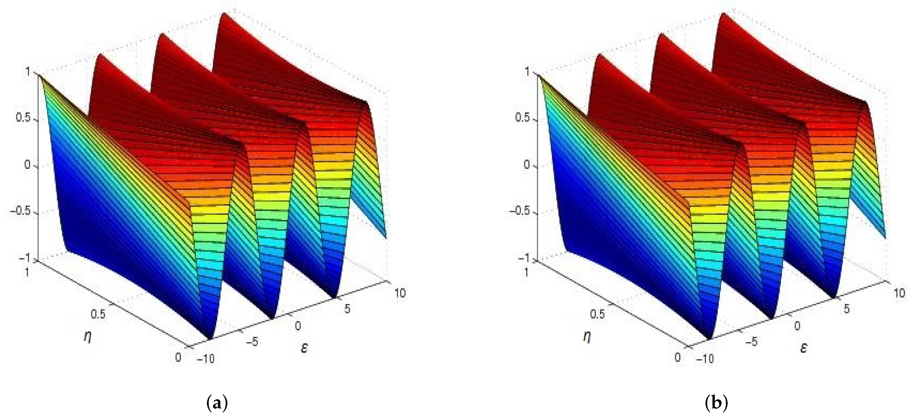
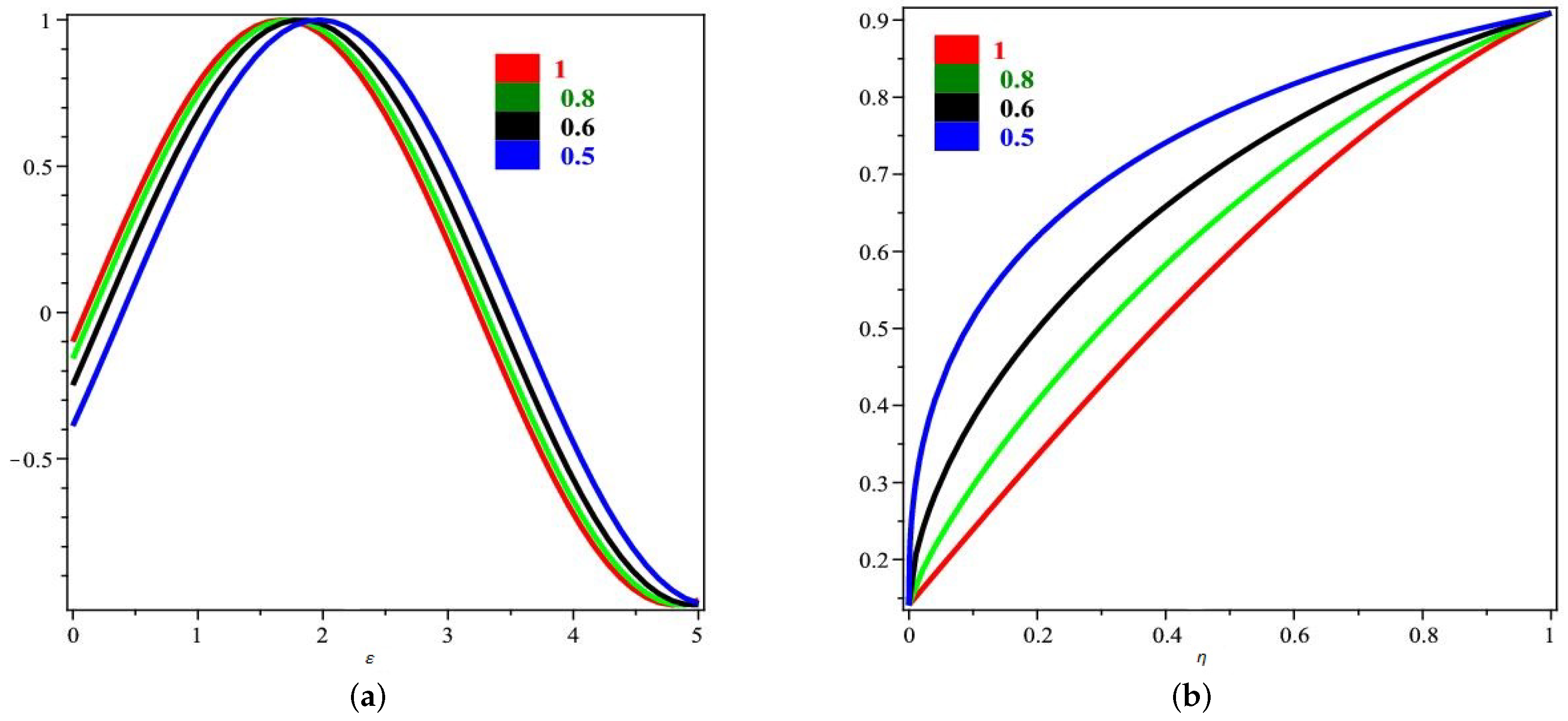
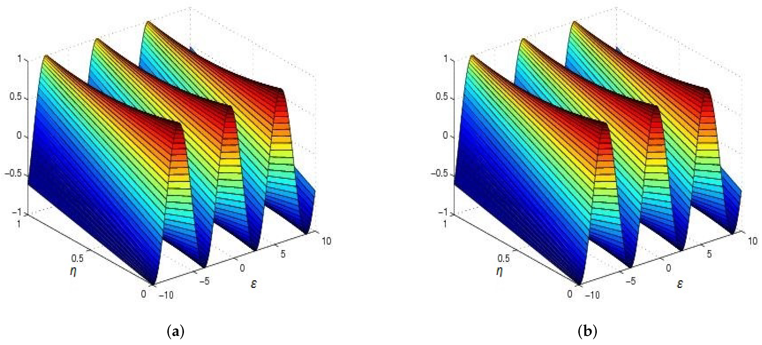
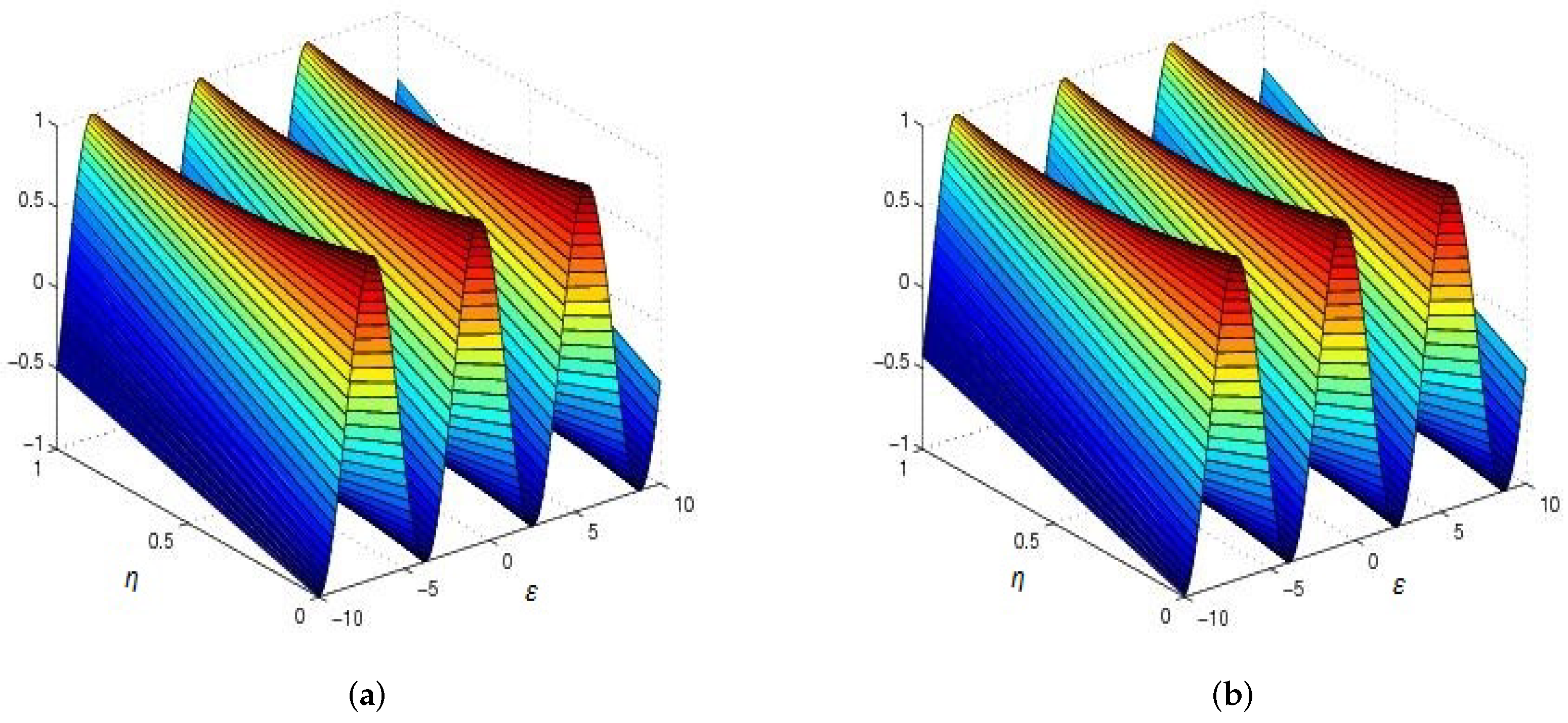
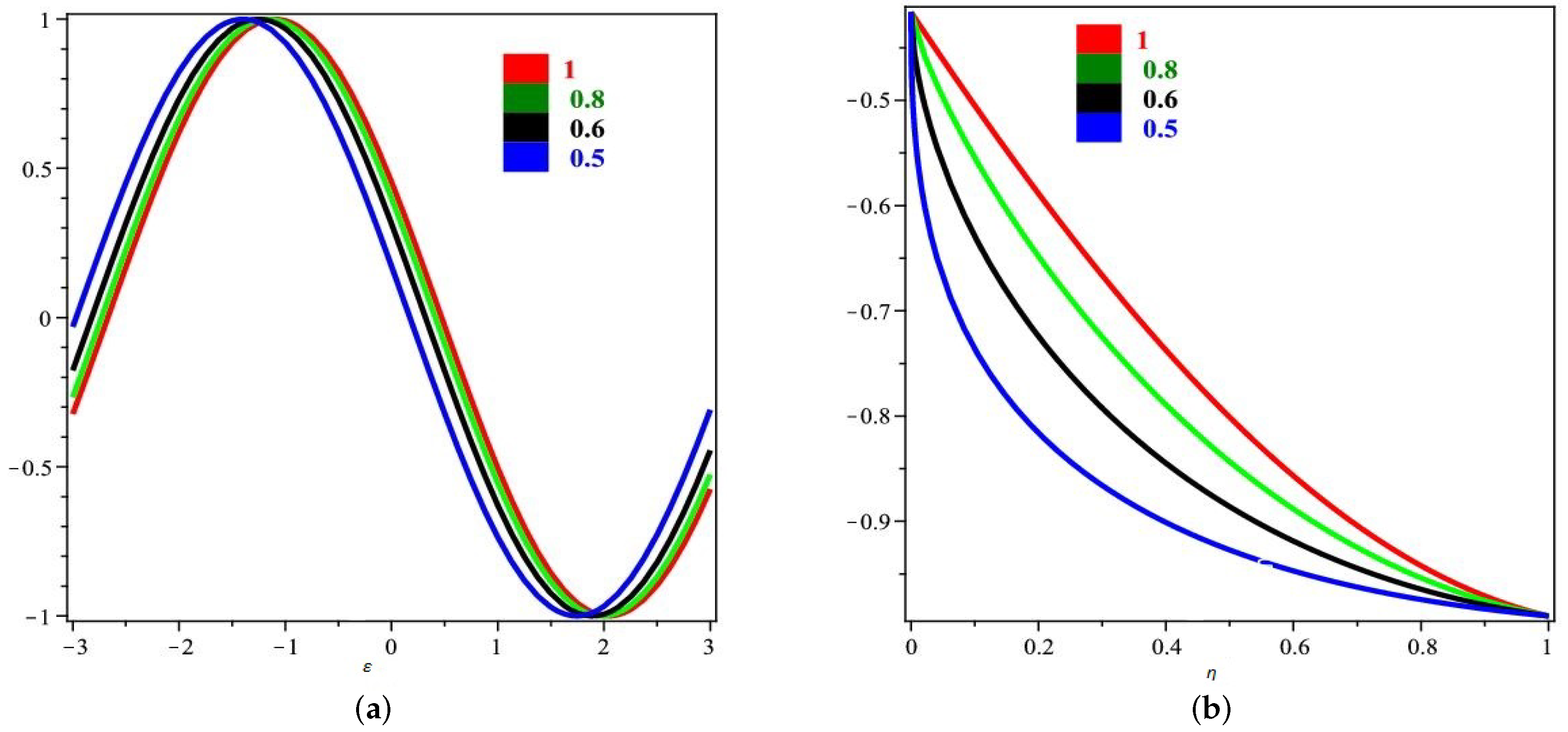
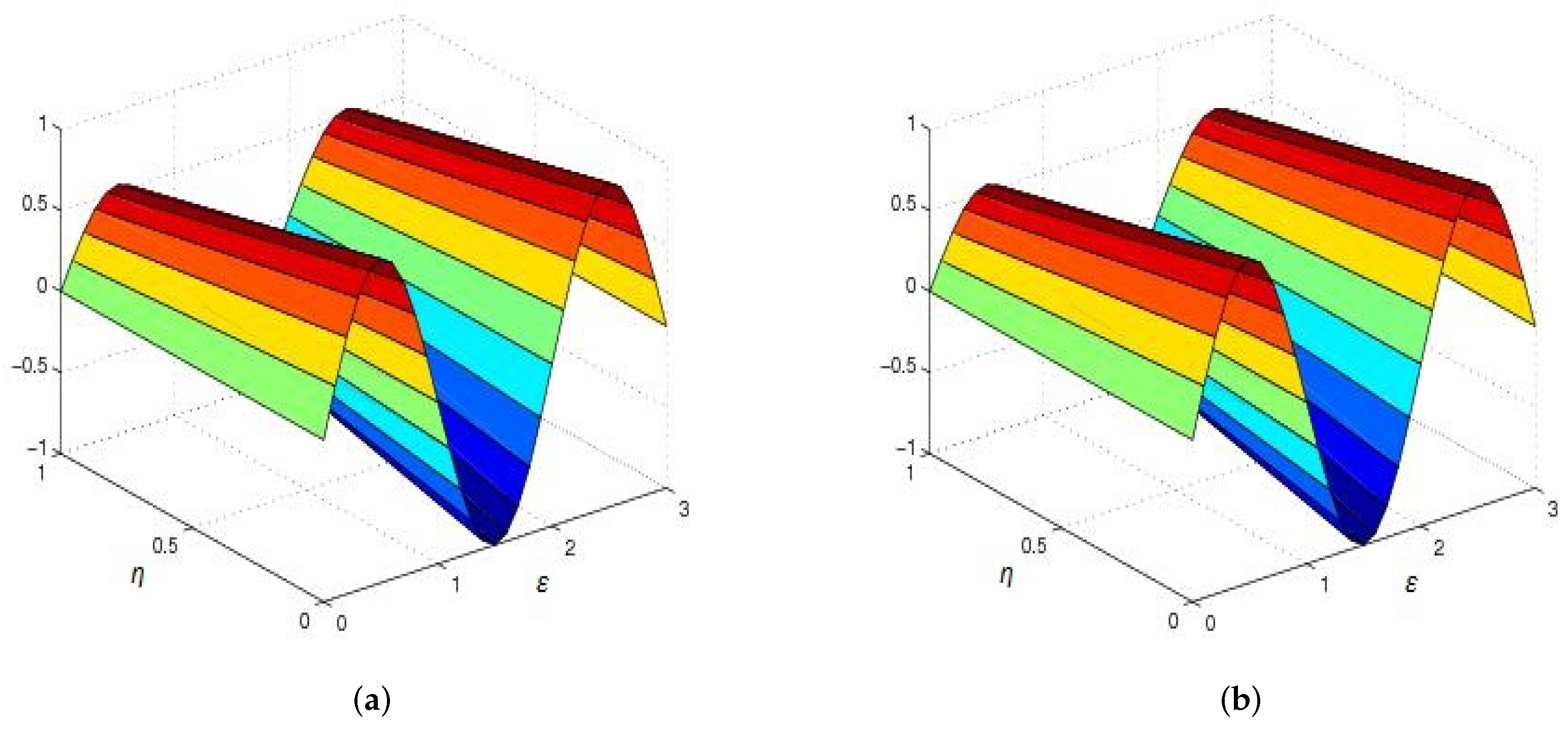
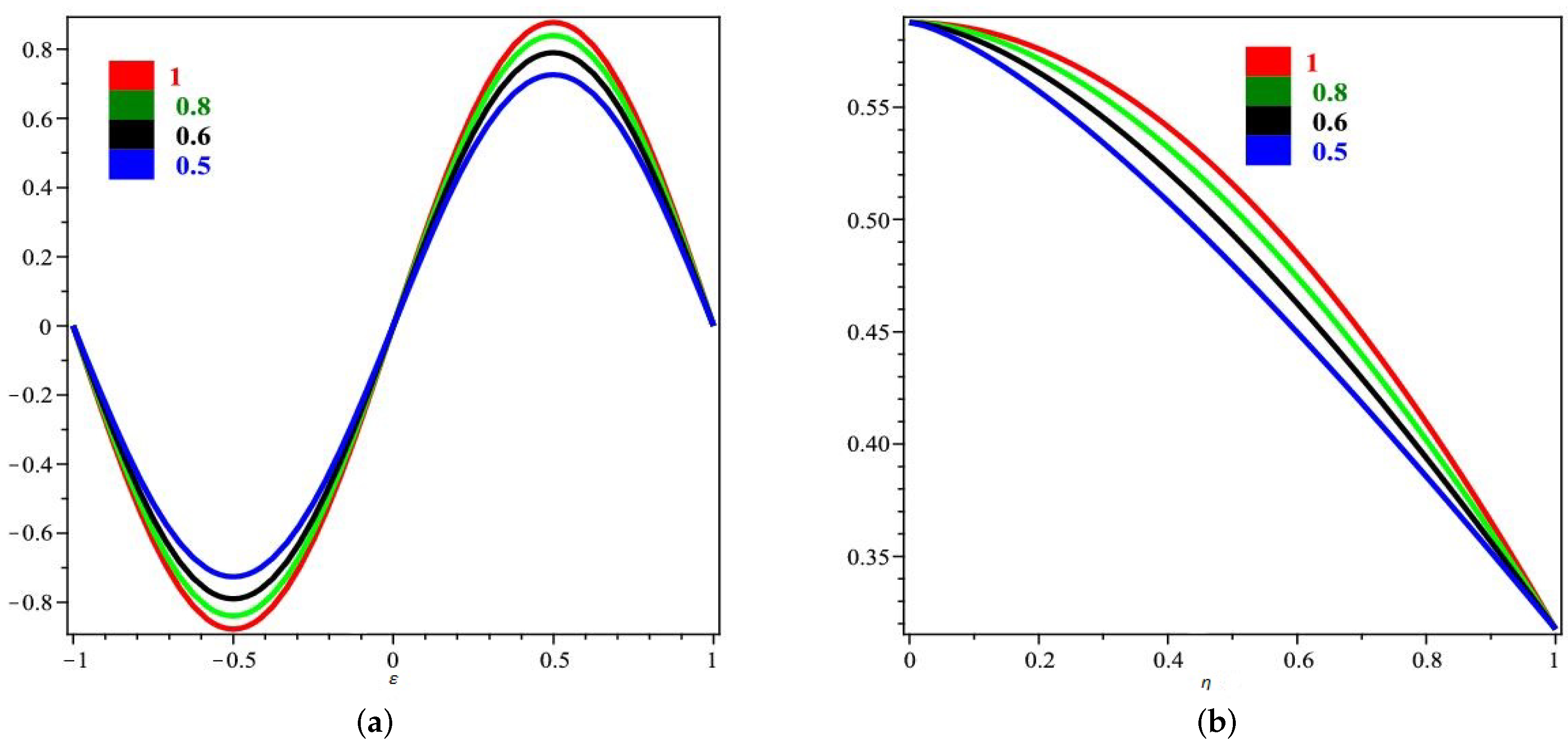
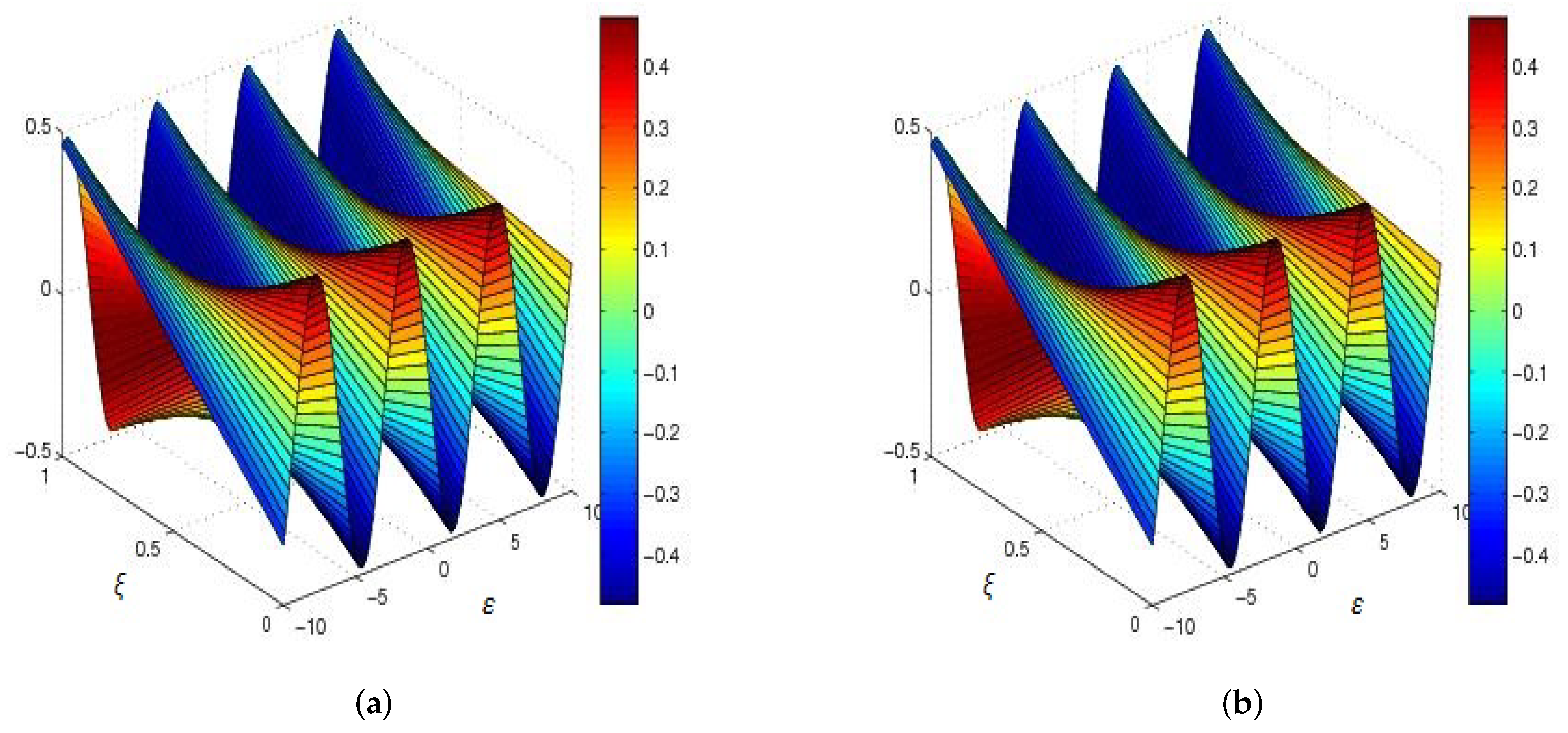
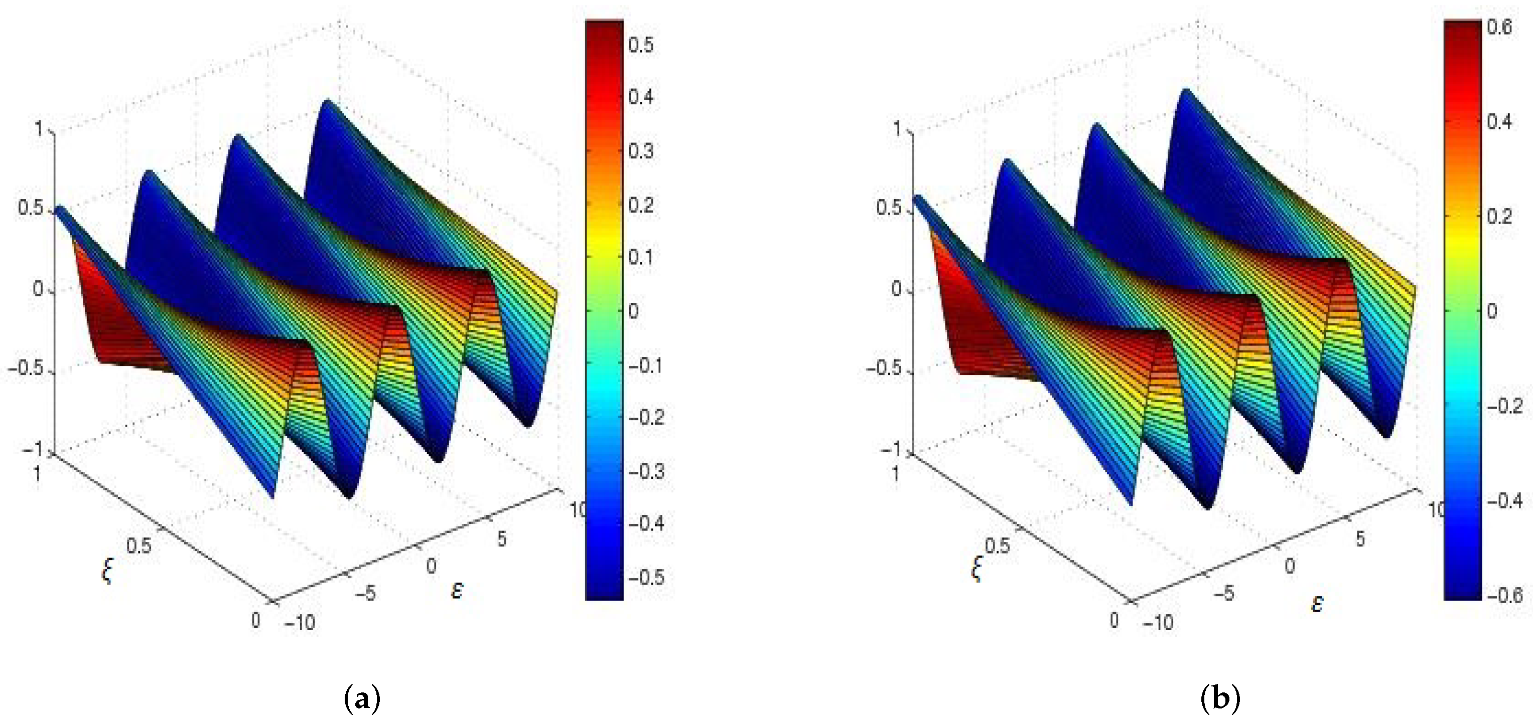
6. Graphical Discussion

The aim this article to investigate an approximate result of the third-order fractional dispersive PDEs, implemented the analytical technique. The new iterative transformation method is applied to analysis of the given problems. The validity show of the suggested method, the result to some illustrative equations are suggested. In Figure 1, (a) the exact result graph of Example 1 at $\delta =1$ and (b) the approximate result graph of $\delta =1$. In Figure 2, (a) the the NITM result of Example 1 at different fractional-order of $\delta =1$ with respective to $ϵ$ and (b) the different fractional-order solution at $\delta =1,0.8,0.6$ and $0.4$ with respect to $\eta$. It is analyzed that the NITM and actual result is in close contact with the exact solution of the propose problem. Also in Figure 3, (a) the exact and (b) NITM solutions plot of Example 2, In Figure 4, (a) and (b) show that are different fractional-order $\gamma =0.8$ and $0.6$. In Figure 5, (a) the the NITM result of Example 2 at different fractional-order of $\delta =1$ with respective to $ϵ$ and (b) the analytical solution of different fractional-order of $\delta =1,0.8,0.6$ and $0.4$ with respect to $\eta$. A similar graphical analysis and discussion can be made for the solutions of Examples 3 and 4 shown in Figure 6, Figure 7, Figure 8 and Figure 9. It has been demonstrated that the suggested methods are similarly accurate It is analyzed whether fractional-order problems, like fractional-order observation, converge to an integer-order result. In

Table 1. $\phi (\epsilon ,\xi ,\eta )$ Comparison of Exact solution, Our methods solution and Absolute Error (AE) of Example 4.

$\mathit{\eta }=0.01$	Exact Solution	Our Methods Soltion	AE of Our Methods	AE of Our Methods	AE of Our Methods
$(\mathbf{\epsilon },\mathbf{\psi })$	$\mathbf{\delta }=\mathbf{1}$	$\mathbf{\delta }=\mathbf{1}$	$\mathbf{\delta }=\mathbf{1}$	$\mathbf{\delta }=\mathbf{0}.\mathbf{9}$	$\delta =0.8$
0	0.000000000000	0.000000000000	0.000000000	0.000000000	0.000000000
0.1	0.03908475646	0.03908475647	8.4147098480$\times {10}^{-12}$	5.8916348320$\times {10}^{-6}$	6.0179783350$\times {10}^{-5}$
0.2	0.07777899096	0.07777899098	1.6829419700$\times {10}^{-11}$	1.1724408770$\times {10}^{-5}$	1.1975827680$\times {10}^{-4}$
0.3	0.11569608350	0.11569608350	0.0000000000	1.7440075190$\times {10}^{-5}$	1.7814016480$\times {10}^{-4}$
0.4	0.15245717900	0.15245717900	0.0000000000	2.2981414070$\times {10}^{-5}$	2.3474221550$\times {10}^{-4}$
0.5	0.18769497280	0.18769497280	8.4147098480$\times {10}^{-11}$	2.8293115510$\times {10}^{-5}$	2.8899866580$\times {10}^{-4}$
0.6	0.22105738040	0.22105738040	0.0000000000	3.3322251000$\times {10}^{-5}$	3.4036760840$\times {10}^{-4}$
0.7	0.25221105580	0.25221105590	8.4147098480$\times {10}^{-11}$	3.8018332270$\times {10}^{-5}$	3.8833574600$\times {10}^{-4}$
0.8	0.28084472170	0.28084472170	8.4147098480$\times {10}^{-11}$	4.2334573540$\times {10}^{-5}$	4.3242369270$\times {10}^{-4}$
0.9	0.30667227990	0.30667228000	8.4147098480$\times {10}^{-11}$	4.6227807340$\times {10}^{-5}$	4.7219102240$\times {10}^{-4}$
1.0	0.32943567010	0.32943567020	8.4147098480$\times {10}^{-11}$	4.9659157730$\times {10}^{-5}$	5.0724039260$\times {10}^{-4}$

show that absolute error of different fractional order represent close contact with each other. The convergence of fractional-order solutions to integral-order approaches is observed in the same way.

7. Conclusions

The iterative transform approach is used to solve fractional-order third-order dispersive partial differential equations in this paper. The resulting findings’ graphical representations have been completed. The improved accuracy of the recommended procedure is clearly demonstrated by this depiction of the acquired findings. The solutions obtained for fractional systems are closely akin to their exact result. It has been demonstrated that fractional answers may be converted to integer-order solutions. The proposed method’s key themes include fewer computations and improved precision. It was later developed to solve various fractional-order linear and nonlinear partial differential equations by the researchers.

References

1. Carpinteri, A.; Mainardi, F. Fractals and Fractional Calculus in Continuum Mechanics; Springer: Wien, NY, USA, 1997. [Google Scholar]
2. Miller, K.S.; Ross, B. An Introduction to the Fractional Calculus and Fractional Differential Equations; Wiley: New York, NY, USA, 1993. [Google Scholar]
3. Shah, R.; Farooq, U.; Khan, H.; Baleanu, D.; Kumam, P.; Arif, M. Fractional View Analysis of Third Order Kortewege-De Vries Equations, Using a New Analytical Technique. Front. Phys. 2020, 7. [Google Scholar] [CrossRef] [Green Version]
4. Shah, R.; Khan, H.; Farooq, U.; Baleanu, D.; Kumam, P.; Arif, M. A New Analytical Technique to Solve System of Fractional-Order Partial Differential Equations. IEEE Access 2019, 7, 150037–150050. [Google Scholar] [CrossRef]
5. Oldham, K.B.; Spanier, J. The Fractional Calculus; Academic Press: New York, NY, USA, 1974. [Google Scholar]
6. Podlubny, I. Fractional Differential Equations; Academic Press: San Diego, CA, USA, 1999. [Google Scholar]
7. Yildirim, E.N.; Akgul, A.; Inc, M. Reproducing kernel method for the solutions of non-linear partial differential equations. Arab. J. Basic Appl. Sci. 2021, 28, 80–86. [Google Scholar] [CrossRef]
8. Qu, H.; She, Z.; Liu, X. Homotopy Analysis Method for Three Types of Fractional Partial Differential Equations. Complexity 2020, 2020, 7232907. [Google Scholar] [CrossRef]
9. Shah, R.; Khan, H.; Baleanu, D.; Kumam, P.; Arif, M. The analytical investigation of time-fractional multi-dimensional Navier–Stokes equation. Alex. Eng. J. 2020, 59, 2941–2956. [Google Scholar] [CrossRef]
10. Okposo, N.I.; Veeresha, P.; Okposo, E.N. Solutions for time-fractional coupled nonlinear Schrodinger equations arising in optical solitons. Chin. J. Phys. 2021, in press. [Google Scholar] [CrossRef]
11. Shah, R.; Khan, H.; Baleanu, D. Fractional Whitham-Broer-Kaup equations within modified analytical approaches. Axioms 2019, 8, 125. [Google Scholar] [CrossRef] [Green Version]
12. Akinyemi, L.; Nisar, K.S.; Saleel, C.A.; Rezazadeh, H.; Veeresha, P.; Khater, M.M.; Inc, M. Novel approach to the analysis of fifth-order weakly nonlocal fractional Schrodinger equation with Caputo derivative. Results Phys. 2021, 31, 104958. [Google Scholar] [CrossRef]
13. Gomez-Aguilar, J.F.; Yepez-Martinez, H.; Torres-Jimenez, J.; Cordova-Fraga, T.; Escobar-Jimenez, R.F.; Olivares-Peregrino, V.H. Homotopy perturbation transform method for nonlinear differential equations involving to fractional operator with exponential kernel. Adv. Differ. Equ. 2017, 2017, 68. [Google Scholar] [CrossRef] [Green Version]
14. Jafari, H.; Khalique, C.M.; Nazari, M. Application of the Laplace decomposition method for solving linear and nonlinear fractional diffusion-wave equations. Appl. Math. Lett. 2011, 24, 1799–1805. [Google Scholar] [CrossRef] [Green Version]
15. Abdou, M.A.; Owyed, S.; Ray, S.S.; Chu, Y.M.; Inc, M.; Ouahid, L. Fractal Ion Acoustic Waves of the Space-Time Fractional Three Dimensional KP Equation. Adv. Math. Phys. 2020, 2020, 8323148. [Google Scholar] [CrossRef]
16. Ali, I.; Khan, H.; Shah, R.; Baleanu, D.; Kumam, P.; Arif, M. Fractional view analysis of acoustic wave equations, using fractional-order differential equations. Appl. Sci. 2020, 10, 610. [Google Scholar] [CrossRef] [Green Version]
17. Alderremy, A.A.; Khan, H.; Shah, R.; Aly, S.; Baleanu, D. The analytical analysis of time-fractional Fornberg-Whitham equations. Mathematics 2020, 8, 987. [Google Scholar] [CrossRef]
18. Baeumer, B.; Benson, D.A.; Meerschaert, M.M.; Wheatcraft, S.W. Subordinated advection-dispersion equation for contaminant transport. Water Resour. Res. 2001, 37, 1543–1550. [Google Scholar] [CrossRef]
19. Benson, D.A.; Wheatcraft, S.W.; Meerschaert, M.M. Application of a fractional advection-dispersion equation. Water Resour. Res. 2000, 36, 1403–1412. [Google Scholar] [CrossRef] [Green Version]
20. Shah, N.A.; Seikh, A.H.; Chung, J.D. The Analysis of Fractional-Order Kersten-Krasil Shchik Coupled KdV System, via a New Integral Transform. Symmetry 2021, 13, 1592. [Google Scholar] [CrossRef]
21. Sunthrayuth, P.; Zidan, A.; Yao, S.; Shah, R.; Inc, M. The Comparative Study for Solving Fractional-Order Fornberg–Whitham Equation via ρ-Laplace Transform. Symmetry 2021, 13, 784. [Google Scholar] [CrossRef]
22. Yang, X.J.; Machado, J.T.; Srivastava, H.M. A new numerical technique for solving the local fractional diffusion equation: Two-dimensional extended differential transform approach. Appl. Math. Comput. 2016, 274, 143–151. [Google Scholar] [CrossRef]
23. Su, W.H.; Yang, X.J.; Jafari, H.; Baleanu, D. Fractional complex transform method for wave equations on Cantor sets within local fractional differential operator. Adv. Differ. Equ. 2013, 2013, 97. [Google Scholar] [CrossRef] [Green Version]
24. Yang, X.J.; Tenreiro Machado, J.A.; Baleanu, D.; Cattani, C. On exact traveling-wave solutions for local fractional Korteweg-de Vries equation. Chaos Interdiscip. J. Nonlinear Sci. 2016, 26, 084312. [Google Scholar] [CrossRef]
25. Sokhanvar, E.; Askari-Hemmat, A.; Yousefi, S.A. Legendre multiwavelet functions for numerical solution of multi-term time-space convection-diffusion equations of fractional order. Eng. Comput. 2021, 37, 1473–1484. [Google Scholar] [CrossRef]
26. Wang, L.; Ma, Y.; Meng, Z. Haar wavelet method for solving fractional partial differential equations numerically. Appl. Math. Comput. 2014, 227, 66–76. [Google Scholar] [CrossRef]
27. Jafari, H.; Seifi, S. Solving a system of nonlinear fractional partial differential equations using homotopy analysis method. Commun. Nonlinear Sci. Numer. Simul. 2009, 14, 1962–1969. [Google Scholar] [CrossRef]
28. Jafari, H.; Nazari, M.; Baleanu, D.; Khalique, C.M. A new approach for solving a system of fractional partial differential equations. Comput. Math. Appl. 2013, 66, 838–843. [Google Scholar] [CrossRef]
29. Baseri, A.; Babolian, E.; Abbasbandy, S. Normalized Bernstein polynomials in solving space-time fractional diffusion equation. Adv. Differ. Equ. 2017, 2017, 346. [Google Scholar] [CrossRef] [Green Version]
30. Jafari, H.; Daftardar-Gejji, V. Solving linear and nonlinear fractional diffusion and wave equations by Adomian decomposition. Appl. Math. Comput. 2006, 180, 488–497. [Google Scholar] [CrossRef]
31. Chen, Y.; Sun, Y.; Liu, L. Numerical solution of fractional partial differential equations with variable coefficients using generalized fractional-order Legendre functions. Appl. Math. Comput. 2014, 244, 847–858. [Google Scholar] [CrossRef]
32. Hajipour, M.; Jajarmi, A.; Baleanu, D. On the accurate discretization of a highly nonlinear boundary value problem. Numer. Algorithms 2018, 79, 679–695. [Google Scholar] [CrossRef]
33. Hajipour, M.; Jajarmi, A.; Malek, A.; Baleanu, D. Positivity-preserving sixth-order implicit finite difference weighted essentially non-oscillatory scheme for the nonlinear heat equation. Appl. Math. Comput. 2018, 325, 146–158. [Google Scholar] [CrossRef]
34. Odibat, Z.; Momani, S. The variational iteration method: An efficient scheme for handling fractional partial differential equations in fluid mechanics. Comput. Math. Appl. 2009, 58, 2199–2208. [Google Scholar] [CrossRef] [Green Version]
35. Nuruddeen, R.I. Elzaki decomposition method and its applications in solving linear and nonlinear Schrodinger equations. Sohag J. Math. 2017, 4, 1–5. [Google Scholar] [CrossRef]
36. Nazari, D.; Shahmorad, S. Application of the fractional differential transform method to fractional-order integro-differential equations with nonlocal boundary conditions. J. Comput. Appl. Math. 2010, 234, 883–891. [Google Scholar] [CrossRef] [Green Version]
37. Khan, H.; Shah, R.; Kumam, P.; Arif, M. Analytical solutions of fractional-order heat and wave equations by the natural transform decomposition method. Entropy 2019, 21, 597. [Google Scholar] [CrossRef] [PubMed] [Green Version]
38. Goswami, A.; Singh, J.; Kumar, D. Numerical simulation of fifth order KdV equations occurring in magneto-acoustic waves. Ain Shams Eng. J. 2018, 9, 2265–2273. [Google Scholar] [CrossRef]
39. Jarad, F.; Abdeljawad, T. A modifi ed Laplace transform for certain generalized fractional operators. Results Nonlinear Anal. 2018, 1, 88–98. [Google Scholar]
40. Bhalekar, S.; Daftardar-Gejji, V. Convergence of the new iterative method. Int. J. Differ. Equ. 2011, 2011, 989065. [Google Scholar] [CrossRef]
41. Shah, R.; Khan, H.; Arif, M.; Kumam, P. Application of Laplace-Adomian decomposition method for the analytical solution of third-order dispersive fractional partial differential equations. Entropy 2019, 21, 335. [Google Scholar] [CrossRef] [Green Version]
Figure 1. (a) The actual result plot of Example 3.1. (b) The approximate result plot of Example 1.
Mathematics 10 00816 g001
Figure 2. (a) The NITM solution graph of different fractional-order δ of Example 1. (b) The NITM solution graph of different fractional-order δ of Example 1.
Mathematics 10 00816 g002
Figure 3. (a) The actual result graph of Example 2. (b) The approximate result plot of Example 2.
Mathematics 10 00816 g003
Figure 4. (a) NITM graph at fractional-order δ = 1.8 of Example 2. (b) NITM plot at fractional-order δ = 1.6 of Example 2.
Mathematics 10 00816 g004
Figure 5. (a) The analytical solution graph of different fractional-order δ of Example 2. (b) The analytical solution graph of different fractional-order δ of Example 2.
Mathematics 10 00816 g005
Figure 6. (a) The actual solution graph of Example 3. (b) The analytical result of figure of Example 3.
Mathematics 10 00816 g006
Figure 7. (a) The analytical solution graph of different fractional-order δ of Example 3. (b) The analytical solution graph of different fractional-order δ of Example 3.
Mathematics 10 00816 g007
Figure 8. (a) The actual result graph Example 4. (b) The analytical result of plot of Example 4.
Mathematics 10 00816 g008
Figure 9. (a) The analytical solution of fractional-order graph δ = 1.8 of Example 4. (b) The analytical solution of fractional-order graph δ = 1.6 of Example 4.
Mathematics 10 00816 g009