The Impact of the Wiener Process on the Analytical Solutions of the Stochastic (2+1)-Dimensional Breaking Soliton Equation by Using Tanh–Coth Method

Abstract

The stochastic (2+1)-dimensional breaking soliton equation (SBSE) is considered in this article, which is forced by the Wiener process. To attain the analytical stochastic solutions such as the polynomials, hyperbolic and trigonometric functions of the SBSE, we use the tanh–coth method. The results provided here extended earlier results. In addition, we utilize Matlab tools to plot 2D and 3D graphs of analytical stochastic solutions derived here to show the effect of the Wiener process on the solutions of the breaking soliton equation.

1. Introduction

Deterministic nonlinear evolution equations (NLEEs) were widely utilized to illustrate some nonlinear phenomena in quantum mechanics, solid-state physics, fluid mechanics, chemical kinematics, plasma physics, the heat flow, optical fibres, etc. Researchers have attempted to find analytic solutions to understand the mechanisms of these phenomena. Therefore, many effective analytical and numerical methods have been proposed by a diverse group of physicists and mathematicians. The Hirota’s [1], Riccati–Bernoulli sub-ODE [2], $exp(-\varphi (\varsigma \left)\right)$-expansion [3], perturbation [4,5,6,7], $(G^{\prime }/G)$-expansion [8,9], Jacobi elliptic function [10], sine–cosine [11,12], tanh–sech [13,14], etc, are some examples of analytical methods. While, a few numerical methods for solving fractional stochastic partial differential equations have been introduced including Galerkin finite element method [15], the meshless method [16,17], finite element method [18], implicit Euler method [19,20], the modified decomposition technique [21], and so on.

In recent years, the validity of including random effects in the study, prediction and simulation of complex phenomena has gained widespread recognition in physics, geophysics, climatic dynamics, biology, chemistry, and other fields. Under noise or random effects, partial differential equations are perfect mathematical problems to represent the complex systems.

It appears to be more crucial to study the NLEEs with some random force. Therefore, we consider here the SBSE in this form [22]:

$$d{\phi }_x-[4{\phi }_x{\phi }_{xy}+2{\phi }_{xx}{\phi }_y-{\phi }_{xxxy}]dt=\sigma {\phi }_{x}d\beta ,$$

(1)

where $\phi$ is a real stochastic function, $\sigma$ is the noise intensity, $\beta$ is the Brownian motion in one variable t, and ${\phi }_{x}d\beta$ is the multiplicative noise in the itô sense.

Many authors have obtained the analytical solutions of the deterministic breaking soliton equation by various methods such as the three-wave [23], Hirota bilinear [24], $\left(\frac{G^{\prime }}{G}\right)$-expansion [25], generalized auxiliary equation [26], tanh–coth [27], improved $\left(\frac{G^{\prime }}{G}\right)$-expansion and extended tanh [28], Jacobi elliptic functions [29], and projective Riccati equation expansion [30]. The solutions to stochastic breaking soliton equations have not been obtained till now.

Our motivation for this work is to acquire the analytical stochastic solutions of the SBSE (1), which has never been considered before in the presence of a stochastic term. To achieve these solutions, we employ the tanh–coth method. Due to the relevance of this equation, which is used to describe the hydrodynamic wave model of shallow-water waves, plasma physics, and the leading flow of fluid, these analytical stochastic solutions are more extensive and crucial in explaining numerous extremely sophisticated physical phenomena. Moreover, the acquired analytical solutions of the SBSE (1) in this article expand several earlier acquired results, such as the result mentioned in [27,28]. We also go over the effects of Wiener process on the analytical solutions of the SBSE (1) via MATLAB tools to display some graphical representations.

This article’s structure is as follows: To obtain the wave equation of the SBSE (1), we use a suitable wave transformation in next section. In Section 3, we apply the tanh–coth method to have the analytical stochastic solution of the SBSE (1). In Section 4, we demonstrate how the Wiener process affects the analytical solutions of the SBSE (1). In Section 5, the physical interpretation is presented. Finally, we provide the article’s conclusions.

2. The Wave Equation of the SBSE

To obtain the wave equation of the SBSE, we employ the next wave transformation:

$$\phi (x,y,t)=\chi \left(\theta \right)e^{(\sigma \beta \left(t\right)-\frac{{\sigma }^2}{2}t)},\theta ={\theta }_{1}x+{\theta }_{2}y+{\theta }_{3}t,$$

(2)

where $\chi$ is a real function, ${\theta }_i$ for all $i=1,2,3$ are constants. We note that:

$$\begin{array}{ccc}\hfill {\phi }_x& =& {\theta }_1{\chi }^{\prime }{e}^{(\sigma \beta \left(t\right)-\frac{{\sigma }^2}{2}t)},\hfill \\ \hfill d{\phi }_x& =& ({\theta }_1{\theta }_3{\chi }^{″}+\frac{1}{2}{\sigma }^2{\theta }_1{\chi }^{\prime }-\frac{1}{2}{\sigma }^2{\theta }_1{\chi }^{\prime })e^{(\sigma \beta \left(t\right)-\frac{{\sigma }^2}{2}t)}dt+\left(\sigma {\theta }_1{\chi }^{\prime }d\beta \right)e^{(\sigma \beta \left(t\right)-\frac{{\sigma }^2}{2}t)},\hfill \\ \hfill \frac{d\phi }{dy}& =& {\theta }_2{\chi }^{\prime }{e}^{(\sigma \beta \left(t\right)-\frac{{\sigma }^2}{2}t)},\frac{d^2\phi }{dxdy}={\theta }_1{\theta }_2{\chi }^{″}{e}^{(\sigma \beta \left(t\right)-\frac{{\sigma }^2}{2}t)},\hfill \\ \hfill \frac{d^2\phi }{d{x}^2}& =& {\theta }_1^2{\chi }^{″}{e}^{(\sigma \beta \left(t\right)-\frac{{\sigma }^2}{2}t)},\frac{d^4\phi }{d{x}^{3}dy}={\theta }_1^3{\theta }_2{\chi }^{⁗}{e}^{(\sigma \beta \left(t\right)-\frac{{\sigma }^2}{2}t)},\hfill \end{array}$$

(3)

where $\frac{1}{2}{\sigma }^{2}dt$ is the Itô correction term. Substituting Equations (2) into (1) and using (3), we obtain the next ordinary differential equation:

$${\theta }_3{\chi }^{″}-6{\theta }_1{\theta }_2{\chi }^{\prime }{\chi }^{″}{e}^{(\sigma \beta \left(t\right)-\frac{{\sigma }^2}{2}t)}+{\theta }_1^2{\theta }_2{\chi }^{⁗}=0.$$

(4)

Recalling that $\chi$ is the deterministic function and taking expectation on both sides of (4), we obtain:

$${\theta }_3{\chi }^{″}-6{\theta }_1{\theta }_2{\chi }^{\prime }{\chi }^{″}{e}^{-\frac{{\sigma }^2}{2}t}\mathbb{E}\left(e^{\sigma \beta \left(t\right)}\right)+{\theta }_1^2{\theta }_2{\chi }^{⁗}=0.$$

(5)

We note for every standard Gaussian process Z that:

$$\mathbb{E}\left(e^{\gamma Z}\right)=e^{\frac{{\gamma }^2}{2}t}$$

(6)

where $\gamma$ is a real number. The identity (6) comes from the fact $\sigma \beta \left(t\right)$ is distributed like $\sigma \sqrt{t}Z.$ Hence, Equation (5) has the following form:

$${\theta }_3{\chi }^{″}-6{\theta }_1{\theta }_2{\chi }^{\prime }{\chi }^{″}+{\theta }_1^2{\theta }_2{\chi }^{⁗}=0.$$

(7)

Integrating Equation (7) once in terms of $\theta ,$ we obtain:

$${\theta }_3{\chi }^{\prime }-3{\theta }_1{\theta }_2{\left[{\chi }^{\prime }\right]}^2+{\theta }_1^2{\theta }_2{\chi }^{‴}=\gamma ,$$

where $\gamma$ is the integration constant. For simplicity, we put $\gamma =0$ to obtain:

$${\theta }_1^2{\theta }_2{\chi }^{‴}+{\theta }_3{\chi }^{\prime }-3{\theta }_1{\theta }_2{\left[{\chi }^{\prime }\right]}^2=0.$$

(8)

Putting

$${\chi }^{\prime }=u,$$

(9)

in Equation (8), we obtain:

$$u^{″}+{\ell }_{1}u-{\ell }_2{u}^2=0,$$

(10)

where

$${\ell }_1=\frac{{\theta }_3}{{\theta }_1^2{\theta }_2}\mathrm{and}{\ell }_2=\frac{3}{{\theta }_1}.$$

3. Tanh–Coth Method

To find the analytical stochastic solutions of the SBSE (1), we employ here the tanh–coth method [14]. Let us define the solution u of (10) as follows:

$$u\left(\theta \right)=\sum _{j=0}^M{a}_k{Y}^j$$

(11)

where $Y=coth\left(\rho \theta \right)$ or $Y=tanh\left(\rho \theta \right)$. Balancing $u^{″}$ with $u^2$ to calculate the parameter M, we obtain:

$$M=2.$$

Rewriting Equation (11) as follows:

$$u\left(\theta \right)=a_0+a_{1}Y+a_2{Y}^2.$$

(12)

Differentiating Equation (12) twice, we have:

$$\begin{array}{ccc}\hfill u^{\prime }& =& \rho a_1+2\rho a_{2}Y-a_1\rho Y^2-2a_2\rho Y^3,\hfill \\ \hfill u^{″}& =& 2{\rho }^2{a}_2-2a_1{\rho }^{2}Y-8a_2{\rho }^2{Y}^2+2a_1{\rho }^2{Y}^3+6a_2{\rho }^2{Y}^4.\hfill \end{array}$$

(13)

Substituting Equations (12) and (13) into Equation (10), we obtain:

$$\begin{array}{ccc}& & (6a_2{\rho }^2-a_2^2{\ell }_2)Y^4+(2a_1{\rho }^2-2a_2{a}_1{\ell }_2)Y^3\hfill \\ & & -(8a_2{\rho }^2+a_1^2{\ell }_2+2a_0{a}_2{\ell }_2-a_2{\ell }_1)Y^2\hfill \end{array}$$

$$-(2a_1{\rho }^2+2a_0{a}_1{\ell }_2-a_1{\ell }_1)Y+(2{\rho }^2{a}_2+a_0{\ell }_1-{\ell }_2{a}_0^2)=0.$$

Equating each coefficient of $Y^j$ to zero for $j=0,1,2,3,4$, we have:

$$(2{\rho }^2{a}_2+a_0{\ell }_1-{\ell }_2{a}_0^2)=0,$$

$$(2a_1{\rho }^2+2a_0{a}_1{\ell }_2-a_1{\ell }_1)=0,$$

$$(8a_2{\rho }^2+a_1^2{\ell }_2+2a_0{a}_2{\ell }_2-a_2{\ell }_1)=0,$$

$$2a_1{\rho }^2-2a_2{a}_1{\ell }_2=0,$$

and

$$(6a_2{\rho }^2-a_2^2{\ell }_2)=0.$$

Solving these equations, we have the next three groups of solutions:

$$a_0=\frac{3{\ell }_1}{2{\ell }_2},a_1=0,a_2=\frac{-3{\ell }_1}{2{\ell }_2},\rho =\frac{1}{2}\sqrt{-{\ell }_1},$$

(14)

$$a_0=\frac{-{\ell }_1}{2{\ell }_2},a_1=0,a_2=\frac{3{\ell }_1}{2{\ell }_2},\mathrm{and}\rho =\frac{1}{2}\sqrt{{\ell }_1},$$

(15)

and

$$a_0=\frac{{\ell }_1}{{\ell }_2},a_1=0,a_2=0,\mathrm{and}\rho =\rho .$$

(16)

For the solutions of Equation (10), the first set (14) provides the following two cases:

Case 1-1: Let ${\ell }_1<0$; then, Equation (10) has the following solutions:

$$u\left(\theta \right)=\frac{3{\ell }_1}{2{\ell }_2}[1-{tanh}^2\left(\frac{1}{2}\sqrt{-{\ell }_1}\theta \right)]=\frac{3{\ell }_1}{2{\ell }_2}sec{h}^2\left(\frac{1}{2}\sqrt{-{\ell }_1}\theta \right),$$

(17)

or

$$u\left(\theta \right)=\frac{3{\ell }_1}{2{\ell }_2}[1-{coth}^2\left(\frac{1}{2}\sqrt{-{\ell }_1}\theta \right)]=\frac{-3{\ell }_1}{2{\ell }_2}csc{h}^2\left(\frac{1}{2}\sqrt{-{\ell }_1}\theta \right).$$

(18)

Integrating Equations (17) and (18) once with respect to $\theta ,$ we obtain:

$${\chi }_{1,1}=\frac{3\sqrt{-{\ell }_1}}{{\ell }_2}tanh\left(\frac{1}{2}\sqrt{-{\ell }_1}\theta \right)+C,$$

(19)

or

$${\chi }_{1,2}=\frac{3\sqrt{-{\ell }_1}}{{\ell }_2}coth\left(\frac{1}{2}\sqrt{-{\ell }_1}\theta \right)+C,$$

(20)

where C is the integral constant. Hence, the analytical stochastic solutions of the SBSE (1) are:

$${\phi }_{1,1}(x,y,t)=[\frac{3\sqrt{-{\ell }_1}}{{\ell }_2}tanh\left(\frac{1}{2}\sqrt{-{\ell }_1}({\theta }_{1}x+{\theta }_{2}y+{\theta }_{3}t)\right)+C]e^{(-\sigma \beta \left(t\right)-\frac{{\sigma }^2}{2}t)},$$

(21)

or

$${\phi }_{1,2}(x,y,t)=[\frac{3\sqrt{-{\ell }_1}}{{\ell }_2}coth\left(\frac{1}{2}\sqrt{-{\ell }_1}({\theta }_{1}x+{\theta }_{2}y+{\theta }_{3}t)\right)+C]e^{(-\sigma \beta \left(t\right)-\frac{{\sigma }^2}{2}t)},$$

(22)

Case 1-2: Let ${\ell }_1>0$, then Equation (10) has the following solutions:

$$u\left(\theta \right)=\frac{3{\ell }_1}{2{\ell }_2}[1+{tan}^2\left(\frac{1}{2}\sqrt{{\ell }_1}\theta \right)]=\frac{3{\ell }_1}{2{\ell }_2}{sec}^2\left(\frac{1}{2}\sqrt{{\ell }_1}\theta \right),$$

(23)

or

$$u\left(\theta \right)=\frac{3{\ell }_1}{2{\ell }_2}[1+{cot}^2\left(\frac{1}{2}\sqrt{{\ell }_1}\theta \right)]=\frac{3{\ell }_1}{2{\ell }_2}{csc}^2\left(\frac{1}{2}\sqrt{{\ell }_1}\theta \right).$$

(24)

Integrating Equations (23) and (24) once with respect to $\theta ,$ we obtain:

$${\chi }_{1,3}=\frac{3\sqrt{{\ell }_1}}{{\ell }_2}tan\left(\frac{1}{2}\sqrt{{\ell }_1}\theta \right)+C,$$

(25)

or

$${\chi }_{1,4}=\frac{-3\sqrt{{\ell }_1}}{{\ell }_2}cot\left(\frac{1}{2}\sqrt{{\ell }_1}\theta \right)+C.$$

(26)

Therefore, the analytical stochastic solutions of the SBSE (1) are:

$${\phi }_{1,3}(x,y,t)=[\frac{3\sqrt{{\ell }_1}}{{\ell }_2}tan\left(\frac{1}{2}\sqrt{{\ell }_1}({\theta }_{1}x+{\theta }_{2}y+{\theta }_{3}t)\right)+C]e^{(\sigma \beta \left(t\right)-\frac{{\sigma }^2}{2}t)},$$

(27)

or

$${\phi }_{1,4}(x,y,t)=[\frac{-3\sqrt{{\ell }_1}}{{\ell }_2}cot\left(\frac{1}{2}\sqrt{{\ell }_1}({\theta }_{1}x+{\theta }_{2}y+{\theta }_{3}t)\right)+C]e^{(\sigma \beta \left(t\right)-\frac{{\sigma }^2}{2}t)}.$$

(28)

The second set (15) provides also two cases as follows:

Case 2-1: Let ${\ell }_1<0$, then Equation (10) has the following solutions:

$$u\left(\theta \right)=\frac{{\ell }_1}{2{\ell }_2}[-1+3{tan}^2\left(\frac{1}{2}\sqrt{-{\ell }_1}\theta \right)]=\frac{{\ell }_1}{2{\ell }_2}[-4+3{sec}^2\left(\frac{1}{2}\sqrt{-{\ell }_1}\theta \right)],$$

(29)

or

$$u\left(\theta \right)=\frac{{\ell }_1}{2{\ell }_2}[-1+3{cot}^2\left(\frac{1}{2}\sqrt{-{\ell }_1}\theta \right)]=\frac{{\ell }_1}{2{\ell }_2}[-4+3{csc}^2\left(\frac{1}{2}\sqrt{-{\ell }_1}\theta \right)],$$

(30)

where $tanh\left(ix\right)=itan\left(x\right)$ and $coth\left(ix\right)=-icot\left(x\right).$

Integrating Equations (29) and (30) once with respect to $\theta ,$ we obtain:

$${\chi }_{2,1}\left(\theta \right)=\frac{{\ell }_1}{{\ell }_2}[-2\theta +\frac{3}{\sqrt{-{\ell }_1}}tan\left(\frac{1}{2}\sqrt{-{\ell }_1}\theta \right)]+C,$$

(31)

or

$${\chi }_{2,2}\left(\theta \right)=\frac{-{\ell }_1}{{\ell }_2}[2\theta -\frac{3}{\sqrt{-{\ell }_1}}cot\left(\frac{1}{2}\sqrt{-{\ell }_1}\theta \right)]+C.$$

(32)

Therefore, the analytical stochastic solutions of the SBSE (1) are

$${\phi }_{2,1}(x,y,t)=[\frac{{\ell }_1}{{\ell }_2}\{-2\theta +\frac{3}{\sqrt{-{\ell }_1}}tan\left(\frac{\sqrt{-{\ell }_1}}{2}\theta \right)\}+C]e^{(\sigma \beta \left(t\right)-\frac{{\sigma }^2}{2}t)},$$

(33)

and

$${\phi }_{2,2}(x,y,t)=\frac{[-{\ell }_1}{{\ell }_2}\{2\theta -\frac{3}{\sqrt{-{\ell }_1}}cot\left(\frac{\sqrt{-{\ell }_1}}{2}\theta \right)\}+C]e^{(\sigma \beta \left(t\right)-\frac{{\sigma }^2}{2}t)},$$

(34)

where $\theta ={\theta }_{1}x+{\theta }_{2}y+{\theta }_{3}t.$

Case 2-2: Let ${\ell }_1>0$, then Equation (10) has the following solutions:

$$u\left(\theta \right)=\frac{{\ell }_1}{2{\ell }_2}[-1+3{tanh}^2\left(\frac{1}{2}\sqrt{{\ell }_1}\theta \right)]=\frac{{\ell }_1}{2{\ell }_2}[2+3sec{h}^2\left(\frac{1}{2}\sqrt{{\ell }_1}\theta \right)],$$

(35)

or

$$u\left(\theta \right)=\frac{{\ell }_1}{2{\ell }_2}[-1+3{coth}^2\left(\frac{1}{2}\sqrt{{\ell }_1}\theta \right)]=\frac{{\ell }_1}{2{\ell }_2}[2+3csc{h}^2\left(\frac{1}{2}\sqrt{{\ell }_1}\theta \right)].$$

(36)

Integrating Equations (17) and (18) once with respect to $\theta ,$ we obtain:

$${\chi }_{2,3}=\frac{{\ell }_1}{{\ell }_2}[\theta +\frac{3}{\sqrt{{\ell }_1}}tanh\left(\frac{1}{2}\sqrt{{\ell }_1}\theta \right)]+C,$$

(37)

or

$${\chi }_{2,4}=\frac{{\ell }_1}{{\ell }_2}[\theta -\frac{3}{\sqrt{{\ell }_1}}coth\left(\frac{1}{2}\sqrt{{\ell }_1}\theta \right)]+C.$$

(38)

Therefore, the analytical stochastic solutions of the SBSE (1) are:

$${\phi }_{2,3}(x,y,t)=[\frac{{\ell }_1}{{\ell }_2}\{\theta +\frac{3}{\sqrt{{\ell }_1}}tanh\left(\frac{1}{2}\sqrt{{\ell }_1}\theta \right)\}+C]e^{(\sigma \beta \left(t\right)-\frac{{\sigma }^2}{2}t)},$$

(39)

and

$${\phi }_{2,4}(x,y,t)=[\frac{{\ell }_1}{{\ell }_2}\{\theta -\frac{3}{\sqrt{{\ell }_1}}coth\left(\frac{1}{2}\sqrt{{\ell }_1}\theta \right)\}+C]e^{(\sigma \beta \left(t\right)-\frac{{\sigma }^2}{2}t)},$$

(40)

where $\theta ={\theta }_{1}x+{\theta }_{2}y+{\theta }_{3}t.$

Meanwhile, the third set (16) gives the solution of Equation (10) as follows:

$$u\left(\theta \right)=\frac{{\ell }_1}{{\ell }_2}.$$

(41)

Integrating Equation (35) once with respect to $\theta ,$ we obtain:

$${\chi }_3\left(\theta \right)=\frac{{\ell }_1}{{\ell }_2}\theta +C.$$

(42)

Therefore, the exact stochastic solutions of the SBSE (1) is

$${\phi }_3(x,y,t)=[\frac{{\ell }_1}{{\ell }_2}({\theta }_{1}x+{\theta }_{2}y+{\theta }_{3}t)+C]e^{(\sigma \beta \left(t\right)-\frac{{\sigma }^2}{2}t)}.$$

(43)

Remark 1.

If we insert $\sigma =0,$ ${\theta }_1={\theta }_2=1$ and ${\theta }_3=-4$ in Equations (21) and (22), then we obtain the same solutions stated in [27] (see Equations (3.10) and (3.11)) and [28] (see, Equation (60)).

Remark 2.

If we insert $\sigma =0,$ ${\theta }_1={\theta }_2=1$ and ${\theta }_3=4$ in Equations (27) and (28), then we obtain the same solutions stated in [28] (see Equations (40) and (61)).

4. The Impact of Wiener Process on the Solutions of SBSE

We demonstrate here the impact of the Wiener process on the analytical solutions of the SBSE (1). The following are some graphs of the behavior of these solutions. We plot the solutions (27), (33) and (39) for various (noise intensity) and fixed parameters ${\theta }_1={\theta }_2=1$ and ${\theta }_3=-4$ (or ${\theta }_3=4)$ by using the MATLAB package, $y=1,$ for $x\in [-5,5]$ and $t\in [0,5],$ as follows:

In the Figure 1, Figure 2 and Figure 3 below, when we look at the surface at $\sigma =0$, we can see that there is some fluctuation and that it is not perfectly flat. However, when the noise is included and its strength increases $\sigma =0.5,1,2$, the surface becomes much more planar after small transit patterns. This shows that the Wiener process affects and stabilizes the solutions.

Finally, in Figure 4, we display a 2D graph of the solution of Equations (27) and (39) with various $\sigma =0,0.5,1,2$ to indicate the impact of the Wiener process on these solutions. We note from Figure 4 that the solution of Equation (1) goes to zero as the noise intensity increases.

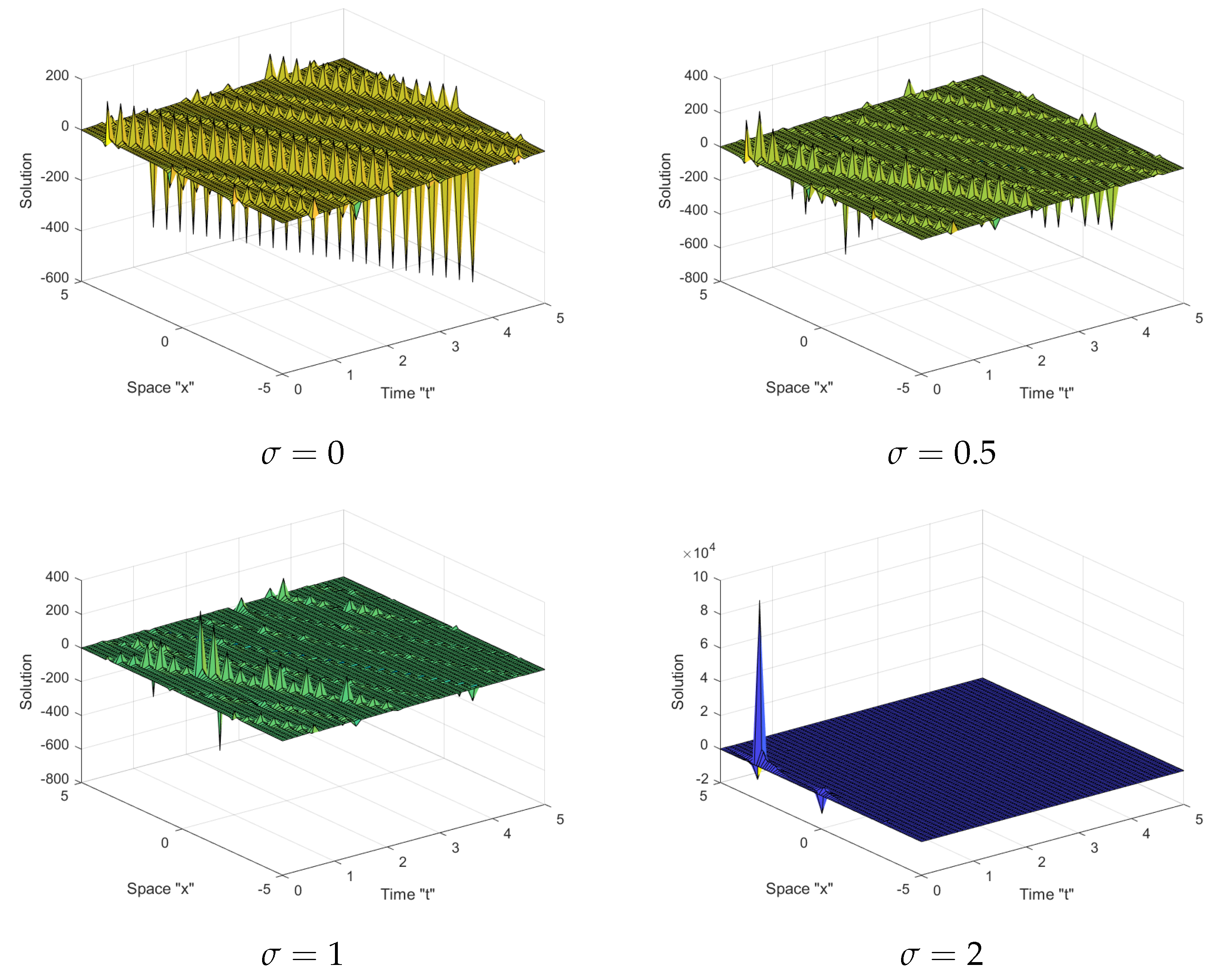
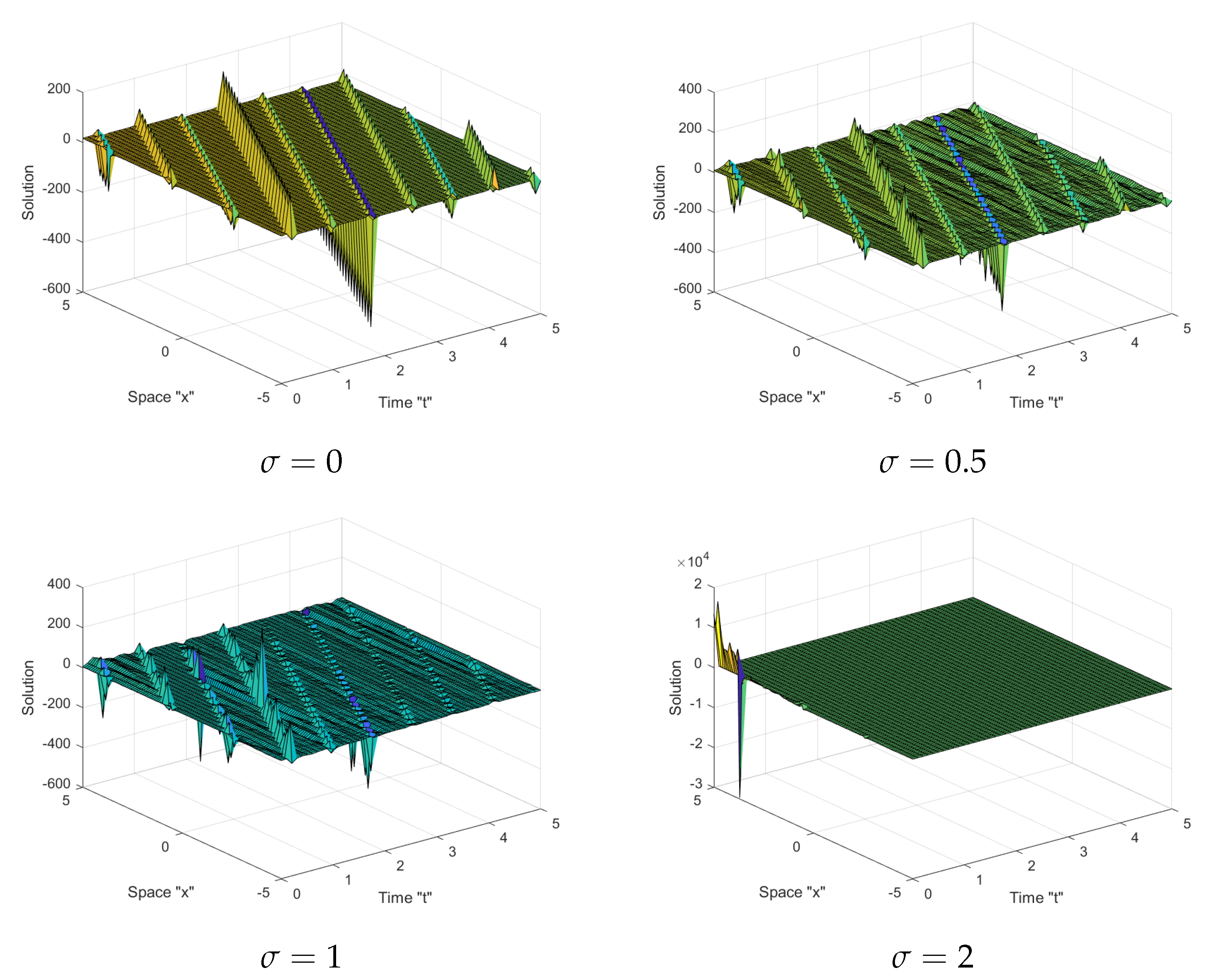
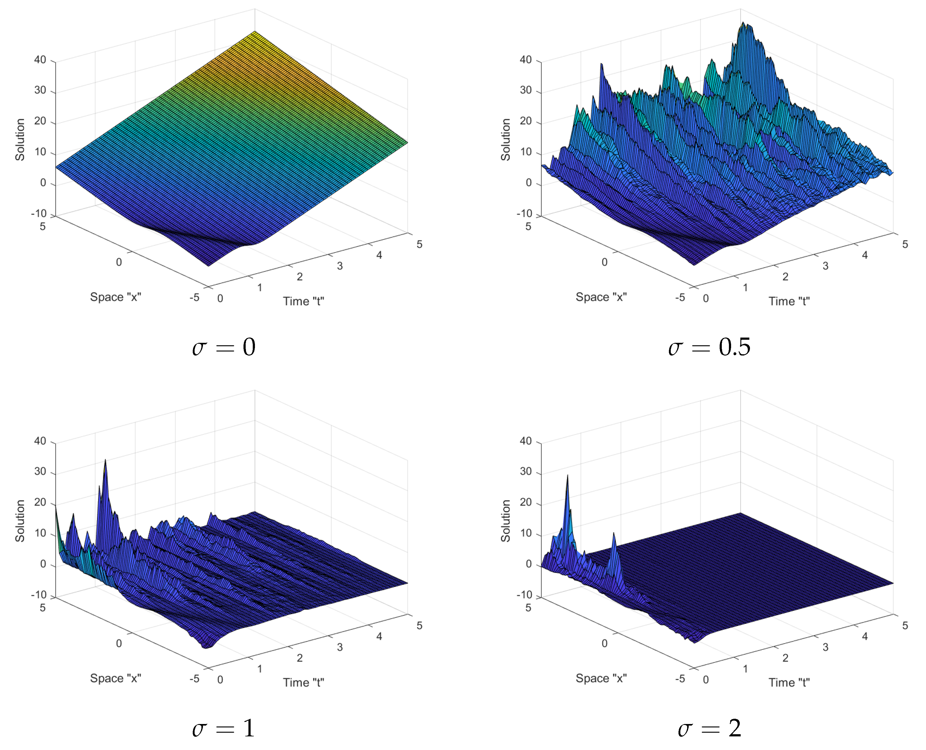
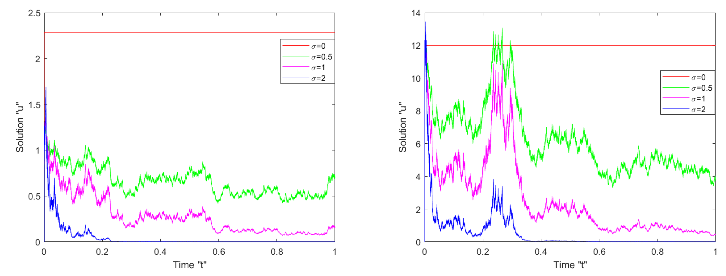
5. Physical Interpretation

The deterministic breaking soliton equation (i.e., (1) with $\sigma =0)$ is utilized to explain the hydrodynamic problem of shallow-water waves, the wave of leading flow of fluid, and plasma physics. The behavior of these waves changes when some external effect (random fluctuations) is considered in (1) as shown in Figure 1, Figure 2 and Figure 3 with $\sigma =0$. As we explained before, the external influence has an impact on the waves and makes them stable as shown in Figure 1, Figure 2 and Figure 3 with $\sigma \ne 0.$

6. Conclusions

In this paper, we got the analytical stochastic solutions including the hyperbolic functions, trigonometric functions, and polynomials for the SBSE (1) via the tanh–coth method. Some previously obtained results were reported in [27,28]. Due to the importance of this equation, which is used to describe the wave of leading fluid flow, plasma physics and the hydrodynamic equation of shallow-water waves, these analytical stochastic solutions are more comprehensive and vital in describing various highly intricate physical phenomena. In the end, we applied the Matlab tools to display the impact of the Wiener process on the obtained solutions of the SBSE, and we deduced that multiplicative Wiener process, in the itô sense, stabilizes the solutions of SBSE. In future studies, we can look at the breaking soliton equation with an additive Wiener process or with a higher dimensional Wiener process.

References

1. Hirota, R. Exact solution of the Korteweg-de Vries equation for multiple collisions of solitons. Phys. Rev. Lett. 1971, 27, 1192–1194. [Google Scholar] [CrossRef]
2. Yang, X.F.; Deng, Z.C.; Wei, Y. A Riccati-Bernoulli sub-ODE method for nonlinear partial differential equations and its application. Adv. Differ. Equ. 2015, 2015, 117–133. [Google Scholar] [CrossRef] [Green Version]
3. Khan, K.; Akbar, M.A. The exp(-ϕ(ς))-expansion method for finding travelling wave solutions of Vakhnenko-Parkes equation. Int. J. Dyn. Syst. Differ. Equ. 2014, 5, 72–83. [Google Scholar]
4. Mohammed, W.W. Approximate solution of the Kuramoto-Shivashinsky equation on an unbounded domain. Chin. Ann. Math. Ser. B 2018, 39, 145–162. [Google Scholar] [CrossRef]
5. Mohammed, W.W. Modulation Equation for the Stochastic Swift–Hohenberg Equation with Cubic and Quintic Nonlinearities on the Real Line. Mathematics 2019, 7, 1217. [Google Scholar] [CrossRef] [Green Version]
6. Mohammed, W.W. Approximate solutions for stochastic time-fractional reaction–diffusion equations with multiplicative noise. Math. Methods Appl. Sci. 2021, 44, 2140–2157. [Google Scholar] [CrossRef]
7. Mohammed, W.W.; Blömker, D. Fast diffusion limit for reaction-diffusion systems with stochastic Neumann boundary conditions. SIAM J. Math. Anal. 2016, 48, 3547–3578. [Google Scholar] [CrossRef] [Green Version]
8. Wang, M.L.; Li, X.Z.; Zhang, J.L. The ( G G )-expansion method and travelling wave solutions of nonlinear evolution equations in mathematical physics. Phys. Lett. A 2008, 372, 417–423. [Google Scholar] [CrossRef]
9. Zhang, H. New application of the ( G G )-expansion method. Commun. Nonlinear Sci. Numer. Simul. 2009, 14, 3220–3225. [Google Scholar] [CrossRef]
10. Yan, Z.L. Abunbant families of Jacobi elliptic function solutions of the-dimensional integrable Davey-Stewartson-type equation via a new method. Chaos Solitons Fractals 2003, 18, 299–309. [Google Scholar] [CrossRef]
11. Wazwaz, A.M. A sine-cosine method for handling nonlinear wave equations. Math. Comput. Model. 2004, 40, 499–508. [Google Scholar] [CrossRef]
12. Yan, C. A simple transformation for nonlinear waves. Phys. Lett. A 1996, 224, 77–84. [Google Scholar] [CrossRef]
13. Wazwaz, A.M. The tanh method: Exact solutions of the Sine–Gordon and Sinh–Gordon equations. Appl. Math. Comput. 2005, 167, 1196–1210. [Google Scholar] [CrossRef]
14. Malfliet, W.; Hereman, W. The tanh method: I. Exact solutions of nonlinear evolution and wave equations. Phys. Scr. 1996, 54, 563–568. [Google Scholar] [CrossRef]
15. Zou, G. Galerkin finite element method for time-fractional stochastic diffusion equations. Comput. Appl. Math. 2018, 37, 4877–4898. [Google Scholar] [CrossRef]
16. Lin, J. Simulation of 2D and 3D inverse source problems of nonlinear time-fractional wave equation by the meshless homogenization function method. Eng. Comput. 2021. [Google Scholar] [CrossRef]
17. Lin, J.; Bai, J.; Reutskiy, S.; Lu, J. A novel RBF-based meshless method for solving time-fractional transport equations in 2D and 3D arbitrary domains. Eng. Comput. 2022. [Google Scholar] [CrossRef]
18. Ford, N.J.; Xiao, J.; Yan, Y. A finite element method for time fractional partial differential equation. Fract. Calc. Aplied Anal. 2011, 14, 454–474. [Google Scholar] [CrossRef] [Green Version]
19. Tambue, A.; Mukam, J.D. Strong convergence of the linear implicit Euler method for the finite element discretization of semilinear SPDEs driven by multiplicative or additive noise. Appl. Math. Comput. 2019, 346, 23–40. [Google Scholar] [CrossRef]
20. Blömker, D.; Mohammed, W.W.; Nolde, C.; Wxoxhrl, F. Numerical study of amplitude equations for SPDEs with degenerate forcing. Int. J. Comput. Math. 2012, 89, 2499–2516. [Google Scholar] [CrossRef]
21. Iqbal, N.; Yasmin, H.; Ali, A.; Bariq, A.; Al-Sawalha, M.M.; Mohammed, W.W. Numerical Methods for Fractional-Order Fornberg-Whitham Equations in the Sense of Atangana-Baleanu Derivative. J. Funct. Spaces 2021, 2021, 2197247. [Google Scholar] [CrossRef]
22. Wazwaz, A.M. Integrable (2+1)-dimensional and (3+1)-dimensional breaking soliton equations. Phys. Scr. 2010, 81, 035005. [Google Scholar] [CrossRef]
23. Darvishi, M.T.; Najafi, M. Some exact solutions of the (2+1)-dimensional breaking soliton equation using the three-wave method. Int. J. Math. Comput. Sci. 2012, 87, 31–34. [Google Scholar]
24. Ilhan, O.P.; Manafian, J. Periodic type and periodic cross-kink wave solutions to the (2+1)-dimensional breaking soliton equation arising in fluid dynamics. Mod. Phys. Lett. B 2019, 33, 1950277. [Google Scholar] [CrossRef]
25. Chen, Y.; Ma, S. Non-Traveling Wave Solutions for the (2+1)-Dimensional Breaking Soliton System. Appl. Math. 2012, 3, 813–818. [Google Scholar] [CrossRef] [Green Version]
26. Zhang, S. New exact non-traveling wave and coefficient function solutions of the (2+1)-dimensional breaking soliton equations. Phys. Lett. A 2007, 368, 470–475. [Google Scholar] [CrossRef]
27. Bekir, A. Exact solutions for some (2+1)-dimensional nonlinear evolution equations by using tanh-coth method. World Appl. Sci. J. 2010, 9, 1–6. [Google Scholar]
28. Akbar, M.A.; Ali, N.H.M.; Mohyud-Din, S.T. Assessment of the further improved ( G G )-expansion method and the extended tanh-method in probing exact solutions ofnonlinear PDEs. SpringerPlus 2013, 2, 326. [Google Scholar] [CrossRef] [PubMed] [Green Version]
29. Peng, Y.-Z. New Exact Solutions for (2+1)-Dimensional Breaking Soliton Equation. Commun. Theor. Phys. 2005, 43, 205–207. [Google Scholar] [CrossRef]
30. Mei, J.Q.; Zhang, H.Q. New types of exact solutions for a breaking soliton equation. Chaos Solitons Fractals 2004, 20, 771. [Google Scholar] [CrossRef]
Figure 1. 3D plot of the obtained solution φ 1 , 3 ( x , 1 , t ) of Equation (27).
Mathematics 10 00817 g001
Figure 2. 3D plot of the obtained solution φ 2 , 1 ( x , 1 , t ) of Equation (33).
Mathematics 10 00817 g002
Figure 3. 3D plot of the obtained solution φ 2 , 3 ( x , 1 , t ) of Equation (39).
Mathematics 10 00817 g003
Figure 4. Two-dimensional plot of the solution of Equations (27) and (39) for different σ = 0 , 0.5 , 1 , 2 .
Mathematics 10 00817 g004
Publisher’s Note: MDPI stays neutral with regard to jurisdictional claims in published maps and institutional affiliations.