
Self-Adaptive Constrained Multi-Objective Differential Evolution Algorithm Based on the State–Action–Reward–State–Action Method


Abstract
:1. Introduction
2. Literature Review
2.1. Constrained Multi-Objective Evolutionary Algorithms
2.2. Self-Adaptive Evolutionary Algorithms
3. Basic Concepts
3.1. Constrained Multi-Objective Optimization Problem
3.2. Concepts in Multi-Objective Optimization Problem
3.3. Constraint Handling Strategies
3.3.1. SP
3.3.2. CDP
- Any feasible solution is preferred to any infeasible solution.
- For two feasible solutions, the Pareto non-dominant individual is preferred.
- For two infeasible solutions, the one with a smaller degree of constraint violation is preferred.
3.3.3. ATM
- The infeasible situation: The constraint violation is considered as an additional objective. The nondominated sorting is applied, and then half of the individuals with fewer constraint violations in the first layer are sorted in the offspring population, then deleted from the population. The same operation is performed on the remaining individuals until the number of offspring reaches population size.
- The semi-feasible situation: Similar to SP, ATM uses a new function, which is calculated as follows:
- The feasible situation: Nondominated sorting is used to select individuals.
3.4. Performance Metric
3.4.1. IGD
3.4.2. HV
3.5. Basics of DE
3.5.1. Generation Strategy
3.5.2. Selection
4. Proposed Algorithm
4.1. Adaptive Constraint Handling Technology
| Algorithm 1: Adaptive Constraint Handling Technique | |
| Input: the state vector SV and the reward chain RC | |
| Output: action chain AC | |
| 1 | Determine the number of individuals selecting each CHT via AC; |
| 2 | Calculate mIGD value according to Equation (12). |
| 3 | Obtain the s′ and r according to mIGD value, and update SV and RC; |
| 4 | Use ε-greedy method to predict individual action a′ according to s′; |
| 5 | Update Q-table: ; |
| 6 | Update action chain AC; |
4.2. Adaptive Generation Strategy
4.3. Overall Implementation of the Proposed Algorithm
| Algorithm 2: ACMODE | |
| Input: Gmax: the maximum number of iterations | |
| Output: final solution set P | |
| 1 | Initialize population ; |
| 2 | Initialize the external archive B, Q-table, the state vector AV and GV, the action chain AC and GC and the reward chain RC and GRC; |
| 3 | for G=1: Gmax do |
| 4 | Each individual selects a F value from the set {0.6, 0.8, 1.0}; |
| 5 | Each individual selects a CR value from the set {0.1, 0.2, 1.0}; |
| 6 | Implement the adaptation of generation strategies according to Section 4.2; |
| 7 | Implement the adaptation of CHTs according to algorithm 1; |
| 8 | Save the feasible solutions at the first level of non-dominated sorting to B; |
| 9 | end for |
| 10 | Output final solution set P according to B. |
5. Experimental Studies
5.1. Benchmark Test Functions and Parameter Settings
5.2. Comparison Results
5.2.1. Comparison Results on CF Test Suite
5.2.2. Comparison Results on LIR-CMOP Test Suite
5.2.3. Comparison Results on NCTP Test Suite
5.2.4. Comparison Results on MW Test Suite
5.2.5. Comparison Results on DAS-CMOP Test Suite
5.2.6. Overall Comparison Results on All Test Suites
5.3. Experimental Analysis
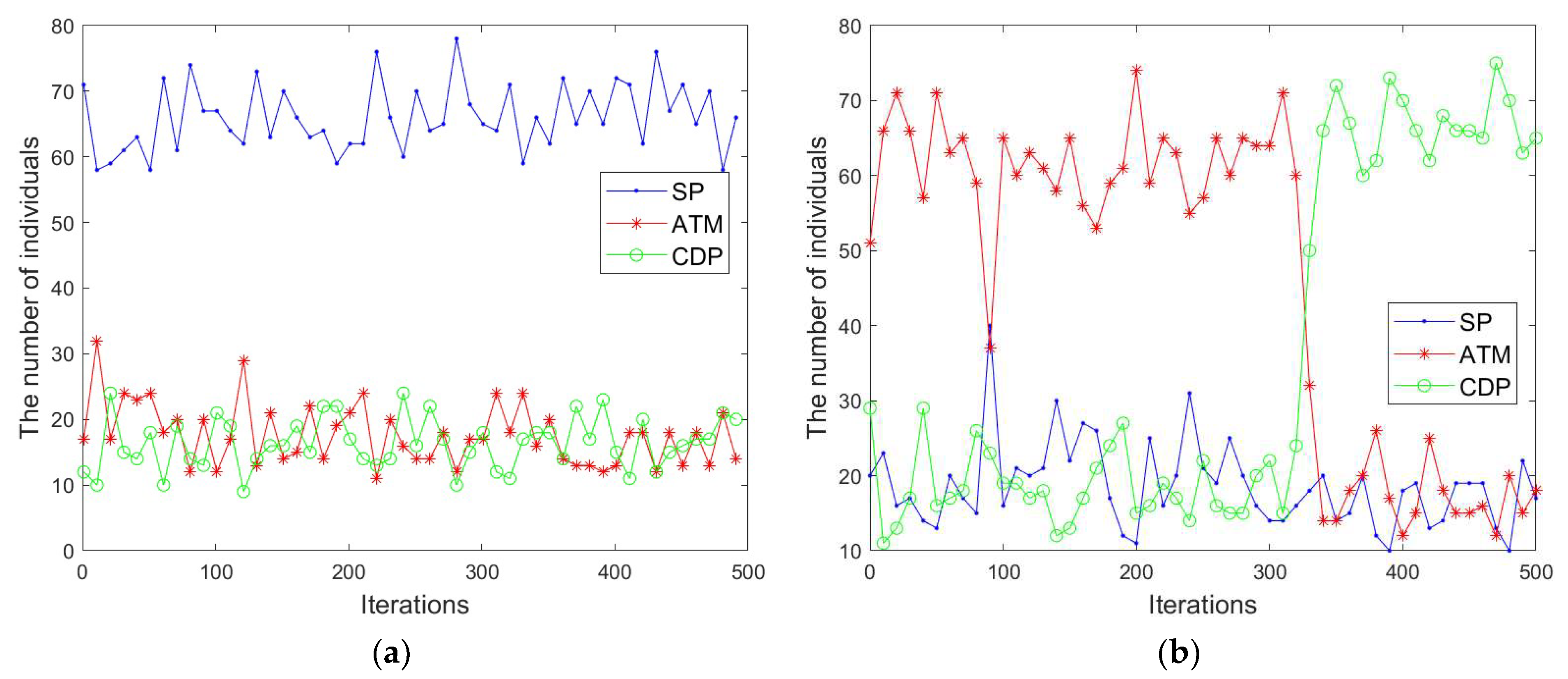
5.3.1. The Effectiveness of Adaptive Constraint Handling Technology
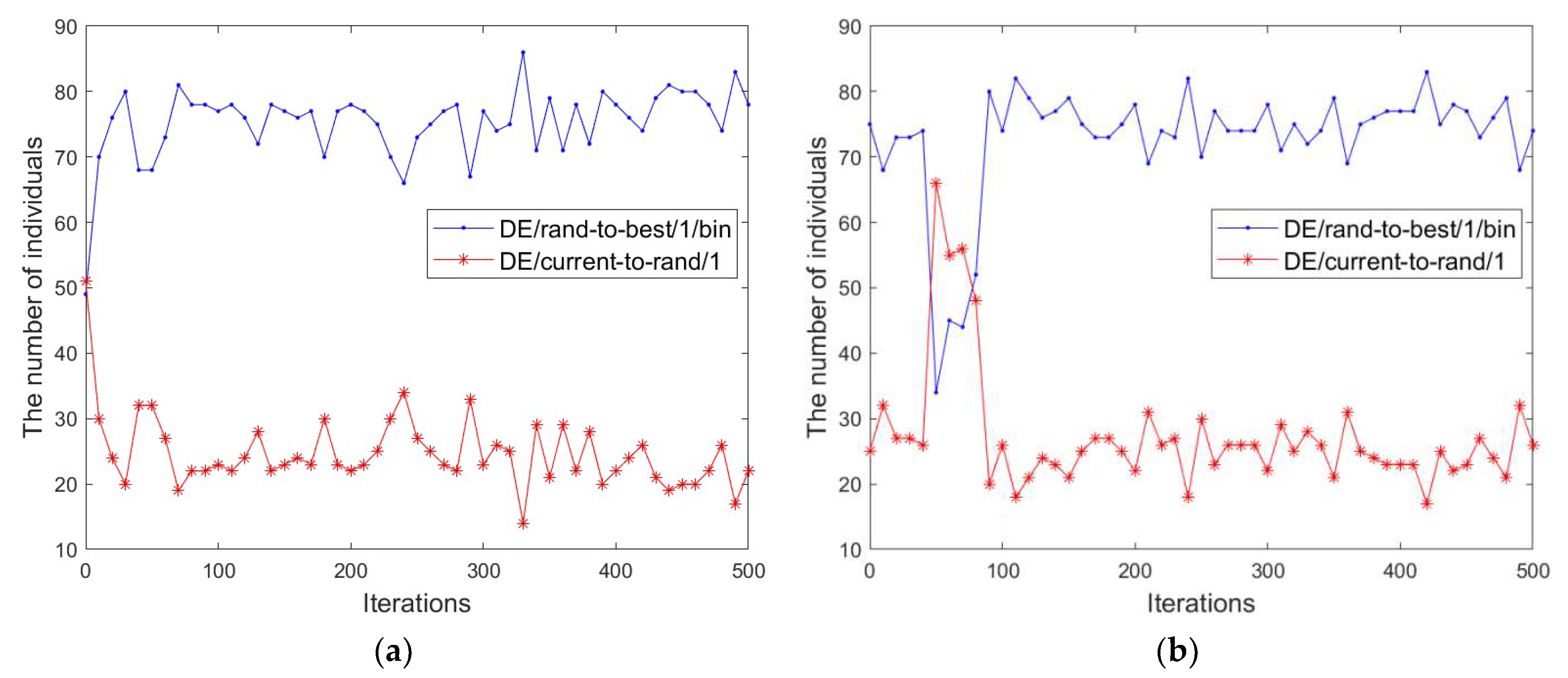
5.3.2. The Effectiveness of Adaptive Generation Strategy
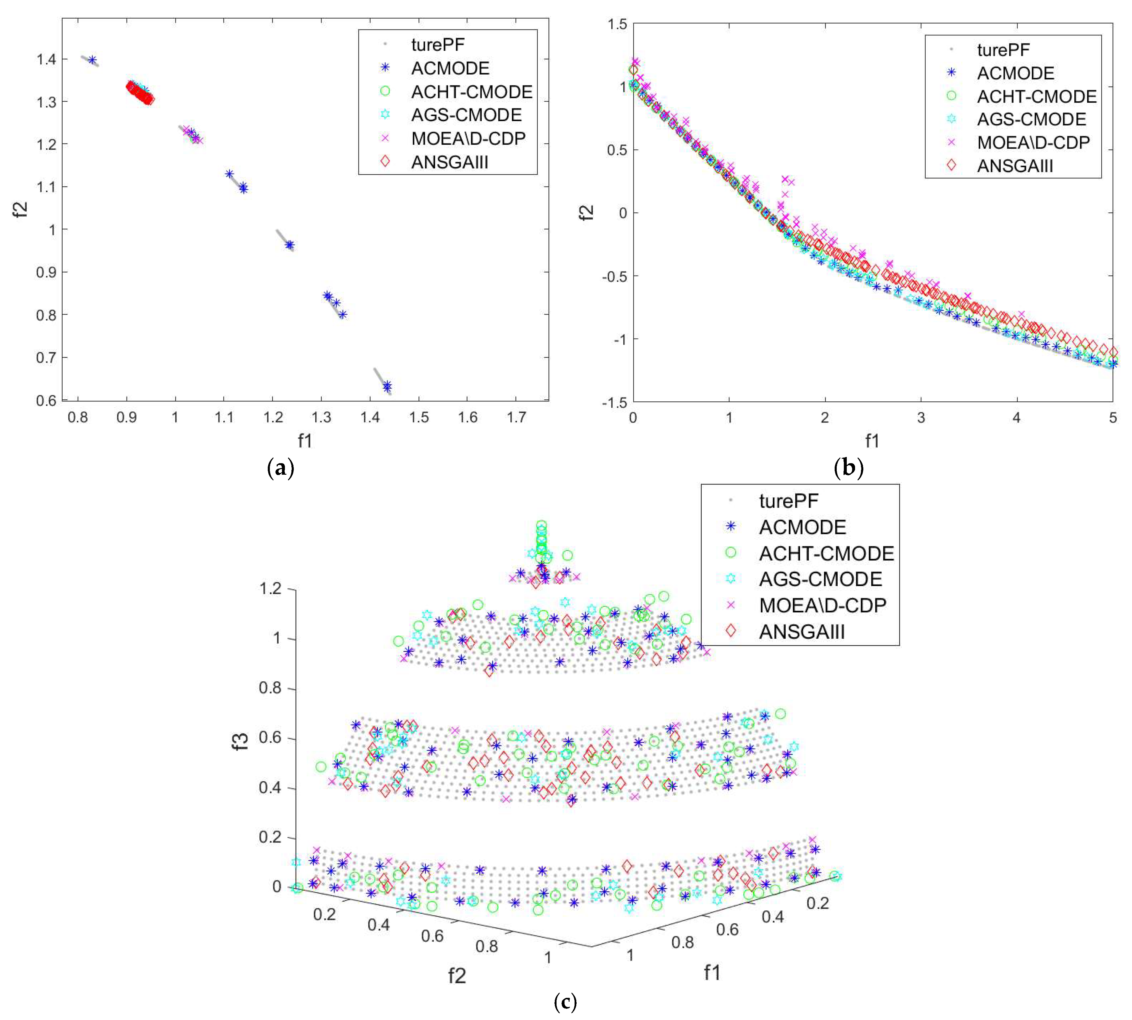
5.3.3. Visual Comparison on PF approximation
5.3.4. Parameter Analysis
6. Discussion
- Compared with the AGS-CMODE, the experimental results show that using adaptive CHTs can assist the proposed algorithm in improving its performance on CMOPs. Moreover, using an adaptive generation strategy can help enhance the performance of the proposed algorithm when compared with the ACHT-CMODE. Therefore, it can be concluded that adaptive CHT and generation strategy is useful for ACOMDE to solve different types of CMOPs.
- MOEA/D-CDP works well on the CMOPs with a low feasibility ratio, and ANSGAIII is a self-adaptive evolutionary algorithm, in which reference points can adaptively update. Compared with these two algorithms, although they are effective on some specific CMOPs, the proposed algorithm outperforms them on most functions.
- The effectiveness of the proposed algorithm is also analyzed. The results demonstrate that the computational resources can be self-adaptively allocated to different CHTs and DE’s generation strategies via the SARSA method during the entire evolutionary process.
7. Conclusions
Author Contributions
Funding
Institutional Review Board Statement
Informed Consent Statement
Data Availability Statement
Acknowledgments
Conflicts of Interest
References
- Maminov, A.; Posypkin, M. Constrained Multi-objective Robot’s Design Optimization. In Proceedings of the 2020 IEEE Conference of Russian Young Researchers in Electrical and Electronic Engineering (EIConRus), St. Petersburg, Russia, 27–30 January 2020; pp. 1992–1995. [Google Scholar]
- Liu, J.; Yang, Y.; Tan, S.; Wang, H. Application of Constrained Multi-objective Evolutionary Algorithm in a Compressed-air Station Scheduling Problem. In Proceedings of the 2019 Chinese Control Conference (CCC), Guangzhou, China, 27–30 July 2019; pp. 2023–2028. [Google Scholar]
- Li, B.; Wang, J.; Xia, N. Dynamic Optimal Scheduling of Microgrid Based on ε constraint multi-objective Biogeography-based Optimization Algorithm. In Proceedings of the 2020 5th International Conference on Automation, Control and Robotics Engineering (CACRE), Dalian, China, 19–20 September 2020; pp. 389–393. [Google Scholar]
- Wang, J.; Li, Y.; Zhang, Q.; Zhang, Z.; Gao, S. Cooperative Multiobjective Evolutionary Algorithm With Propulsive Population for Constrained Multiobjective Optimization. IEEE Trans. Syst. Man Cybern. Syst. 2021, 1–16. [Google Scholar] [CrossRef]
- Datta, R.; Deb, K.; Segev, A. A bi-objective hybrid constrained optimization (HyCon) method using a multi-objective and penalty function approach. In Proceedings of the 2017 IEEE Congress on Evolutionary Computation (CEC), Donostia-San Sebastián, Spain, 5–8 June 2017; pp. 317–324. [Google Scholar]
- Yuan, J.; Liu, H.L.; Ong, Y.S.; He, Z. Indicator-based Evolutionary Algorithm for Solving Constrained Multi-objective Optimization Problems. IEEE Trans. Evol. Comput. 2021, 1. [Google Scholar] [CrossRef]
- Cui, C.X.; Fan, Q.Q. Constrained Multi-objective Differential Evolutionary Algorithm with Adaptive Constraint Handling Technique. World Sci. Res. J. 2021, 7, 322–339. [Google Scholar] [CrossRef]
- Richard, S.S.; Andrew, G.B. Temporal-Difference Learning. In Reinforcement Learning: An Introduction; MIT Press: Cambridge, MA, USA, 1998; pp. 133–160. [Google Scholar]
- Yu, X.B.; Lu, Y.Q. A corner point-based algorithm to solve constrained multi-objective optimization problems. Appl. Intell. 2018, 48, 3019–3037. [Google Scholar] [CrossRef]
- Xiang, Y.; Yang, X.W.; Huang, H.; Wang, J.H. Balancing Constraints and Objectives by Considering Problem Types in Constrained Multiobjective Optimization. IEEE Trans. Cybern. 2021, 1–14. [Google Scholar] [CrossRef]
- Fan, Z.; Li, W.J.; Cai, X.Y.; Li, H.; Wei, C.M.; Zhang, Q.F.; Deb, K.; Goodman, E. Push and pull search for solving constrained multi-objective optimization problems. Swarm Evol. Comput. 2019, 44, 665–679. [Google Scholar] [CrossRef] [Green Version]
- Uribe, L.; Lara, A.; Deb, K.; Schutze, O. A new gradient free local search mechanism for constrained multi-objective optimization problems. Swarm Evol. Comput. 2021, 67, 100938. [Google Scholar] [CrossRef]
- Liu, Z.Z.; Wang, Y.; Wang, B.C. Indicator-Based Constrained Multiobjective Evolutionary Algorithms. IEEE Trans. Syst. Man Cybern. Syst. 2021, 51, 5414–5426. [Google Scholar] [CrossRef]
- Tian, Y.; Zhang, T.; Xiao, J.; Zhang, X.; Jin, Y. A Coevolutionary Framework for Constrained Multiobjective Optimization Problems. IEEE Trans. Evol. Comput. 2021, 25, 102–116. [Google Scholar] [CrossRef]
- Liu, Z.Z.; Wang, Y. Handling Constrained Multiobjective Optimization Problems With Constraints in Both the Decision and Objective Spaces. IEEE Trans. Evol. Comput. 2019, 23, 870–884. [Google Scholar] [CrossRef]
- Ming, M.; Wang, R.; Ishibuchi, H.; Zhang, T. A Novel Dual-Stage Dual-Population Evolutionary Algorithm for Constrained Multi-Objective Optimization. IEEE Trans. Evol. Comput. 2021, 1. [Google Scholar] [CrossRef]
- Storn, R.; Price, K. Differential evolution—A simple and efficient heuristic for global optimization over continuous spaces. J. Glob. Optim. 1997, 11, 341–359. [Google Scholar] [CrossRef]
- Xu, B.; Duan, W.; Zhang, H.F.; Li, Z.Q. Differential evolution with infeasible-guiding mutation operators for constrained multi-objective optimization. Appl. Intell. 2020, 50, 4459–4481. [Google Scholar] [CrossRef]
- Yu, K.; Liang, J.; Qu, B.; Luo, Y.; Yue, C. Dynamic Selection Preference-Assisted Constrained Multiobjective Differential Evolution. IEEE Trans. Syst. Man Cybern. Syst. 2021, 1–12. [Google Scholar] [CrossRef]
- Yang, Y.K.; Liu, J.C.; Tan, S.B. A partition-based constrained multi-objective evolutionary algorithm. Swarm Evol. Comput. 2021, 66, 100940. [Google Scholar] [CrossRef]
- Lin, Y.; Du, W.; Du, W. Multi-objective differential evolution with dynamic hybrid constraint handling mechanism. Soft Comput. 2019, 23, 4341–4355. [Google Scholar] [CrossRef]
- Yu, X.B.; Yu, X.R.; Lu, Y.Q.; Yen, G.G.; Cai, M. Differential evolution mutation operators for constrained multi-objective optimization. Appl. Soft Comput. 2018, 67, 452–466. [Google Scholar] [CrossRef]
- Wang, J.; Liang, G.; Zhang, J. Cooperative Differential Evolution Framework for Constrained Multiobjective Optimization. IEEE Trans. Cybern. 2019, 49, 2060–2072. [Google Scholar] [CrossRef]
- Moniz, N.; Monteiro, H. No Free Lunch in imbalanced learning. Knowl.-Based Syst. 2021, 227, 107222. [Google Scholar] [CrossRef]
- Yang, Y.K.; Liu, J.C.; Tan, S.B.; Wang, H.H. A multi-objective differential evolutionary algorithm for constrained multi-objective optimization problems with low feasible ratio. Appl. Soft Comput. 2019, 80, 42–56. [Google Scholar] [CrossRef]
- Yang, N.; Liu, H.L. Adaptively Allocating Constraint-Handling Techniques for Constrained Multi-objective Optimization Problems. Int. J. Pattern Recognit. Artif. Intell. 2021, 35, 2159032. [Google Scholar] [CrossRef]
- Liu, B.J.; Bi, X.J. Adaptive ε-Constraint Multi-Objective Evolutionary Algorithm Based on Decomposition and Differential Evolution. IEEE Access 2021, 9, 17596–17609. [Google Scholar] [CrossRef]
- Mashwani, W.K.; Salhi, A.; Yeniay, O.; Jan, M.A.; Khanum, R.A. Hybrid adaptive evolutionary algorithm based on decomposition. Appl. Soft Comput. 2017, 57, 363–378. [Google Scholar] [CrossRef] [Green Version]
- Zhang, L.; Bi, X.J.; Wang, Y.J. Adaptive Truncation technique for Constrained Multi-Objective Optimization. Ksii Trans. Internet Inf. Syst. 2019, 13, 5489–5511. [Google Scholar] [CrossRef]
- Samanipour, F.; Jelovica, J. Adaptive repair method for constraint handling in multi-objective genetic algorithm based on relationship between constraints and variables. Appl. Soft Comput. 2020, 90, 106143. [Google Scholar] [CrossRef]
- Fan, Q.; Zhang, Y.; Li, N. An Autoselection Strategy of Multiobjective Evolutionary Algorithms Based on Performance Indicator and Its Application. IEEE Trans. Autom. Sci. Eng. 2021, 1–15. [Google Scholar] [CrossRef]
- Woldesenbet, Y.G.; Yen, G.G.; Tessema, B.G. Constraint Handling in Multiobjective Evolutionary Optimization. IEEE Trans. Evol. Comput. 2009, 13, 514–525. [Google Scholar] [CrossRef]
- Deb, K.; Pratap, A.; Agarwal, S.; Meyarivan, T. A fast and elitist multiobjective genetic algorithm: NSGA-II. IEEE Trans. Evol. Comput. 2002, 6, 182–197. [Google Scholar] [CrossRef] [Green Version]
- Wang, Y.; Cai, Z.; Zhou, Y.; Zeng, W. An Adaptive Tradeoff Model for Constrained Evolutionary Optimization. IEEE Trans. Evol. Comput. 2008, 12, 80–92. [Google Scholar] [CrossRef]
- Bosman, P.A.N.; Thierens, D. The balance between proximity and diversity in multiobjective evolutionary algorithms. IEEE Trans. Evol. Comput. 2003, 7, 174–188. [Google Scholar] [CrossRef] [Green Version]
- Yuan, J.; Liu, H.-L.; He, Z. A constrained multi-objective evolutionary algorithm using valuable infeasible solutions. Swarm Evol. Comput. 2022, 68, 101020. [Google Scholar] [CrossRef]
- Zitzler, E.; Thiele, L. Multiobjective evolutionary algorithms: A comparative case study and the strength Pareto approach. IEEE Trans. Evol. Comput. 1999, 3, 257–271. [Google Scholar] [CrossRef] [Green Version]
- Fan, Q.; Yan, X.; Zhang, Y.; Zhu, C. A Variable Search Space Strategy Based on Sequential Trust Region Determination Technique. IEEE Trans. Cybern. 2021, 51, 2712–2724. [Google Scholar] [CrossRef] [PubMed]
- Fan, Q.Q.; Wang, W.L.; Yan, X.F. Multi-objective differential evolution with performance-metric-based self-adaptive mutation operator for chemical and qbiochemical dynamic optimization problems. Appl. Soft Comput. 2017, 59, 33–44. [Google Scholar] [CrossRef]
- Shahrabi, J.; Adibi, M.A.; Mahootchi, M. A reinforcement learning approach to parameter estimation in dynamic job shop scheduling. Comput. Ind. Eng. 2017, 110, 75–82. [Google Scholar] [CrossRef]
- Jan, M.A.; Khanum, R.A. A study of two penalty-parameterless constraint handling techniques in the framework of MOEA/D. Appl. Soft Comput. 2013, 13, 128–148. [Google Scholar] [CrossRef]
- Jain, H.; Deb, K. An Evolutionary Many-Objective Optimization Algorithm Using Reference-Point Based Nondominated Sorting Approach, Part II: Handling Constraints and Extending to an Adaptive Approach. IEEE Trans. Evol. Comput. 2014, 18, 602–622. [Google Scholar] [CrossRef]
- Wilcoxon, F. Individual Comparisons by Ranking Methods. Biom. Bull. 1945, 1, 80–83. [Google Scholar] [CrossRef]
- Friedman, M. The Use of Ranks to Avoid the Assumption of Normality Implicit in the Analysis of Variance. J. Am. Stat. Assoc. 1937, 32, 675–701. [Google Scholar] [CrossRef]
- Zhang, Q.; Zhou, A.; Zhao, S.; Suganthan, P.N.; Tiwari, S. Multiobjective optimization Test Instances for the CEC 2009 Special Session and Competition. Mech. Eng. 2008, 264, 1–30. [Google Scholar]
- Fan, Z.; Fang, Y.; Li, W.; Cai, X.; Wei, C.; Goodman, E. MOEA/D with angle-based constrained dominance principle for constrained multi-objective optimization problems. Appl. Soft Comput. J. 2018, 74, 621–633. [Google Scholar] [CrossRef] [Green Version]
- Li, J.P.; Wang, Y.; Yang, S.; Cai, Z. A comparative study of constraint-handling techniques in evolutionary constrained multiobjective optimization. In Proceedings of the 2016 IEEE Congress on Evolutionary Computation (CEC), Vancouver, BC, Canada, 24–29 July 2016; pp. 4175–4182. [Google Scholar]
- Ma, Z.; Wang, Y. Evolutionary Constrained Multiobjective Optimization: Test Suite Construction and Performance Comparisons. IEEE Trans. Evol. Comput. 2019, 23, 972–986. [Google Scholar] [CrossRef]
- Fan, Z.; Li, W.J.; Cai, X.Y.; Li, H.; Wei, C.M.; Zhang, Q.F.; Deb, K.; Goodman, E. Difficulty Adjustable and Scalable Constrained Multiobjective Test Problem Toolkit. Evol. Comput. 2020, 28, 339–378. [Google Scholar] [CrossRef] [PubMed] [Green Version]
- Liu, Y.; Cao, B.; Li, H. Improving ant colony optimization algorithm with epsilon greedy and Levy flight. Complex Intell. Syst. 2021, 7, 1711–1722. [Google Scholar] [CrossRef] [Green Version]


| Q-Table | SP | CDP | ATM |
|---|---|---|---|
| excellent | Q (1,1) | Q (1,2) | Q (1,3) |
| medium | Q (2,1) | Q (2,2) | Q (2,3) |
| poor | Q (3,1) | Q (3,2) | Q (3,3) |
| ACHT-CMODE | AGS-CMODE | MOEA/D-CDP | ANSGAIII | ACMODE | |
|---|---|---|---|---|---|
| CF1 | 5.2867 × 10⁻² | 3.7910 × 10⁻² | 3.7102 × 10⁻² | 3.4372 × 10⁻² | 1.0970 × 10⁻² |
| (7.62 × 10⁻³) − | (1.19 × 10⁻²) − | (4.12 × 10⁻³) − | (3.22 × 10⁻³) − | (1.70 × 10⁻³) | |
| CF2 | 9.0126 × 10⁻² | 3.0672 × 10⁻² | 1.8108 × 10⁻¹ | 8.2723 × 10⁻² | 3.0182 × 10⁻² |
| (3.69 × 10⁻²) − | (1.15 × 10⁻²) = | (5.59 × 10⁻²) − | (4.15 × 10⁻²) − | (1.00 × 10⁻²) | |
| CF3 | 2.9612 × 10⁻¹ | 2.6593 × 10⁻¹ | 3.3179 × 10⁻¹ | 2.2112 × 10⁻¹ | 1.4216 × 10⁻¹ |
| (9.80 × 10⁻²) − | (1.10 × 10⁻¹) − | (1.21 × 10⁻¹) − | (5.41 × 10⁻²) − | (1.11 × 10⁻¹) | |
| CF4 | 7.6876 × 10⁻² | 7.3348 × 10⁻² | 1.6755 × 10⁻¹ | 1.0219 × 10⁻¹ | 7.0695 × 10⁻² |
| (1.79 × 10⁻²) = | (9.28 × 10⁻³) = | (4.40 × 10⁻²) − | (3.14 × 10⁻²) − | (1.01 × 10⁻²) | |
| CF5 | 3.8964 × 10⁻¹ | 2.5490 × 10⁻¹ | 3.7316 × 10⁻¹ | 2.9797 × 10⁻¹ | 2.2979 × 10⁻¹ |
| (1.77 × 10⁻¹) − | (1.02 × 10⁻¹) = | (1.45 × 10⁻¹) − | (1.22 × 10⁻¹) − | (1.41 × 10⁻¹) | |
| CF6 | 6.6338 × 10⁻² | 6.1696 × 10⁻² | 1.7894 × 10⁻¹ | 7.5225 × 10⁻² | 5.0066 × 10⁻² |
| (2.31 × 10⁻²) − | (2.76 × 10⁻²) − | (5.31 × 10⁻²) − | (2.96 × 10⁻²) − | (2.14 × 10⁻²) | |
| CF7 | 3.0948 × 10⁻¹ | 2.5622 × 10⁻¹ | 4.1771 × 10⁻¹ | 3.2974 × 10⁻¹ | 2.1991 × 10⁻¹ |
| (1.59 × 10⁻¹) − | (1.86 × 10⁻¹) = | (1.62 × 10⁻¹) − | (1.25 × 10⁻¹) − | (1.20 × 10⁻¹) | |
| CF8 | 4.0369 × 10⁻¹ | 3.2016 × 10⁻¹ | NaN | NaN | 3.0085 × 10⁻¹ |
| (1.01 × 10⁻¹) − | (2.46 × 10⁻²) − | (NaN) | (NaN) | (3.02 × 10⁻²) | |
| CF9 | 2.2998 × 10⁻¹ | 1.9144 × 10⁻¹ | 1.6194 × 10⁻¹ | 1.9518 × 10⁻¹ | 1.6347 × 10⁻¹ |
| (2.75 × 10⁻²) − | (1.63 × 10⁻²) − | (2.33 × 10⁻²) = | (1.08 × 10⁻¹) = | (2.48 × 10⁻²) | |
| CF10 | 4.8295 × 100 | 6.1970 × 10⁻¹ | NaN | NaN | 5.8169 × 10⁻¹ |
| (4.96 × 100) − | (8.87 × 10⁻²) = | (NaN) | (NaN) | (9.69 × 10⁻²) | |
| +/=/− | 0/1/9 | 0/5/5 | 0/1/9 | 0/1/9 | / |
| ACHT-CMODE | AGS-CMODE | MOEA/D-CDP | ANSGAIII | ACMODE | |
|---|---|---|---|---|---|
| CF1 | 5.0226 × 10⁻¹ | 5.3020 × 10⁻¹ | 5.1961 × 10⁻¹ | 5.2354 × 10⁻¹ | 5.5277 × 10⁻¹ |
| (7.44 × 10⁻³) − | (1.35 × 10⁻²) − | (4.77 × 10⁻³) − | (4.12 × 10⁻³) − | (2.06 × 10⁻³) | |
| CF2 | 6.1541 × 10⁻¹ | 6.3414 × 10⁻¹ | 5.5158 × 10⁻¹ | 5.9870 × 10⁻¹ | 6.3741 × 10⁻¹ |
| (2.87 × 10⁻²) − | (1.64 × 10⁻²) = | (3.16 × 10⁻²) − | (2.31 × 10⁻²) − | (1.21 × 10⁻²) | |
| CF3 | 1.4263 × 10⁻¹ | 6.2928 × 10⁻² | 1.4502 × 10⁻¹ | 1.6713 × 10⁻¹ | 2.2932 × 10⁻¹ |
| (4.49 × 10⁻²) − | (5.37 × 10⁻²) − | (3.71 × 10⁻²) − | (3.70 × 10⁻²) − | (6.97 × 10⁻²) | |
| CF4 | 4.1802 × 10⁻¹ | 4.2951 × 10⁻¹ | 3.6115 × 10⁻¹ | 4.1346 × 10⁻¹ | 4.4357 × 10⁻¹ |
| (2.82 × 10⁻²) − | (1.88 × 10⁻²) − | (3.64 × 10⁻²) − | (3.10 × 10⁻²) − | (1.33 × 10⁻²) | |
| CF5 | 1.7365 × 10⁻¹ | 2.1278 × 10⁻¹ | 2.5767 × 10⁻¹ | 2.6832 × 10⁻¹ | 3.0478 × 10⁻¹ |
| (1.16 × 10⁻¹) − | (7.31 × 10⁻²) − | (7.95 × 10⁻²) − | (6.40 × 10⁻²) − | (8.62 × 10⁻²) | |
| CF6 | 6.3664 × 10⁻¹ | 6.4217 × 10⁻¹ | 5.9050 × 10⁻¹ | 6.3067 × 10⁻¹ | 6.5454 × 10⁻¹ |
| (1.30 × 10⁻²) − | (1.17 × 10⁻²) − | (3.13 × 10⁻²) − | (1.78 × 10⁻²) − | (1.13 × 10⁻²) | |
| CF7 | 3.0291 × 10⁻¹ | 4.5368 × 10⁻¹ | 3.6811 × 10⁻¹ | 4.2346 × 10⁻¹ | 4.8571 × 10⁻¹ |
| (1.75 × 10⁻¹) − | (1.14 × 10⁻¹) = | (1.18 × 10⁻¹) − | (7.56 × 10⁻²) − | (8.66 × 10⁻²) | |
| CF8 | 1.6747 × 10⁻¹ | 1.7895 × 10⁻¹ | NaN | NaN | 2.1303 × 10⁻¹ |
| (5.29 × 10⁻²) − | (2.12 × 10⁻²) − | (NaN) | (NaN) | (2.79 × 10⁻²) | |
| CF9 | 3.8431 × 10⁻¹ | 3.3650 × 10⁻¹ | 3.6784 × 10⁻¹ | 3.6594 × 10⁻¹ | 3.9182 × 10⁻¹ |
| (5.47 × 10⁻²) = | (3.04 × 10⁻²) − | (2.87 × 10⁻²) − | (6.20 × 10⁻²) − | (3.27 × 10⁻²) | |
| CF10 | 6.2801 × 10⁻² | 9.8047 × 10⁻² | NaN | NaN | 1.0148 × 10⁻¹ |
| (8.36 × 10⁻²) = | (1.45 × 10⁻²) = | (NaN) | (NaN) | (2.46 × 10⁻²) | |
| +/=/− | 0/2/8 | 0/3/7 | 0/0/10 | 0/0/10 | / |
| ACHT-CMODE | AGS-CMODE | MOEA/D-CDP | ANSGAIII | ACMODE | |
|---|---|---|---|---|---|
| LIR-CMOP1 | 3.6782 × 10⁻¹ | 2.3948 × 10⁻¹ | 2.8261 × 10⁻¹ | 3.1440 × 10⁻¹ | 1.2279 × 10⁻¹ |
| (3.26 × 10⁻²) − | (2.93 × 10⁻²) − | (2.59 × 10⁻²) − | (3.53 × 10⁻²) − | (1.23 × 10⁻¹) | |
| LIR-CMOP2 | 3.1322 × 10⁻¹ | 2.1796 × 10⁻¹ | 2.4263 × 10⁻¹ | 2.6801 × 10⁻¹ | 9.6984 × 10⁻² |
| (4.71 × 10⁻²) − | (4.85 × 10⁻²) − | (2.63 × 10⁻²) − | (2.32 × 10⁻²) − | (9.13 × 10⁻²) | |
| LIR-CMOP3 | 3.5187 × 10⁻¹ | 2.8157 × 10⁻¹ | 2.8272 × 10⁻¹ | 3.1967 × 10⁻¹ | 1.3190 × 10⁻¹ |
| (3.17 × 10⁻²) − | (4.36 × 10⁻²) − | (3.83 × 10⁻²) − | (3.25 × 10⁻²) − | (1.14 × 10⁻¹) | |
| LIR-CMOP4 | 3.2254 × 10⁻¹ | 2.7900 × 10⁻¹ | 2.6684 × 10⁻¹ | 2.9089 × 10⁻¹ | 1.6098 × 10⁻¹ |
| (7.29 × 10⁻³) − | (4.83 × 10⁻²) = | (3.91 × 10⁻²) = | (2.94 × 10⁻²) = | (1.09 × 10⁻¹) | |
| LIR-CMOP5 | 1.2205 × 100 | 1.2156 × 100 | 1.4539 × 100 | 1.2484 × 100 | 1.1738 × 100 |
| (7.48 × 10⁻³) − | (2.33 × 10⁻²) = | (5.10 × 10⁻¹) − | (6.88 × 10⁻²) − | (1.94 × 10⁻¹) | |
| LIR-CMOP6 | 1.3471 × 100 | 1.2726 × 100 | 1.4029 × 100 | 1.3460 × 100 | 1.1320 × 100 |
| (1.02 × 10⁻³) − | (2.38 × 10⁻¹) − | (2.59 × 10⁻¹) = | (3.32 × 10⁻⁴) = | (3.99 × 10⁻¹) | |
| LIR-CMOP7 | 8.4456 × 10⁻¹ | 1.0911 × 100 | 1.5268 × 100 | 1.4345 × 100 | 2.3164 × 10⁻¹ |
| (7.45 × 10⁻¹) − | (7.23 × 10⁻¹) − | (4.09 × 10⁻¹) − | (5.53 × 10⁻¹) − | (2.95 × 10⁻¹) | |
| LIR-CMOP8 | 1.1796 × 100 | 1.2161 × 100 | 1.6403 × 100 | 1.5431 × 100 | 8.1410 × 10⁻¹ |
| (6.73 × 10⁻¹) − | (6.40 × 10⁻¹) − | (2.10 × 10⁻¹) − | (4.10 × 10⁻¹) − | (7.27 × 10⁻¹) | |
| LIR-CMOP9 | 1.0273 × 100 | 5.5734 × 10⁻¹ | 9.0252 × 10⁻¹ | 1.0191 × 100 | 5.3120 × 10⁻¹ |
| (7.07 × 10⁻²) − | (7.24 × 10⁻²) = | (1.10 × 10⁻¹) − | (4.95 × 10⁻²) − | (4.73 × 10⁻²) | |
| LIR-CMOP10 | 9.2893 × 10⁻¹ | 4.4541 × 10⁻¹ | 7.9612 × 10⁻¹ | 1.0207 × 100 | 3.2702 × 10⁻¹ |
| (4.32 × 10⁻²) − | (8.36 × 10⁻²) − | (1.46 × 10⁻¹) − | (5.34 × 10⁻²) − | (7.42 × 10⁻²) | |
| LIR-CMOP11 | 8.9470 × 10⁻¹ | 5.1836 × 10⁻¹ | 8.6793 × 10⁻¹ | 9.2118 × 10⁻¹ | 3.7547 × 10⁻¹ |
| (6.88 × 10⁻²) − | (1.19 × 10⁻¹) − | (8.18 × 10⁻²) − | (7.37 × 10⁻²) − | (1.51 × 10⁻¹) | |
| LIR-CMOP12 | 7.2041 × 10⁻¹ | 3.6486 × 10⁻¹ | 6.8840 × 10⁻¹ | 8.6910 × 10⁻¹ | 3.4246 × 10⁻¹ |
| (1.19 × 10⁻¹) − | (5.08 × 10⁻²) = | (1.64 × 10⁻¹) − | (1.61 × 10⁻¹) − | (5.85 × 10⁻²) | |
| LIR-CMOP13 | 1.3443 × 100 | 1.3369 × 100 | 1.3056 × 100 | 1.3182 × 100 | 1.2505 × 100 |
| (5.97 × 10⁻³) − | (3.90 × 10⁻²) − | (4.43 × 10⁻⁴) − | (4.62 × 10⁻³) − | (2.54 × 10⁻¹) | |
| LIR-CMOP14 | 1.3018 × 100 | 1.2980 × 100 | 1.2618 × 100 | 1.2753 × 100 | 1.2762 × 100 |
| (5.25 × 10⁻³) − | (5.31 × 10⁻³) − | (4.42 × 10⁻⁴) + | (3.67 × 10⁻³) − | (3.77 × 10⁻²) | |
| +/=/− | 0/0/14 | 0/4/10 | 1/2/11 | 0/2/12 |
| ACHT-CMODE | AGS-CMODE | MOEA/D-CDP | ANSGAIII | ACMODE | |
|---|---|---|---|---|---|
| LIR-CMOP-1 | 1.0470 × 10⁻¹ | 1.3078 × 10⁻¹ | 1.1914 × 10⁻¹ | 1.0895 × 10⁻¹ | 1.9034 × 10⁻¹ |
| (7.03 × 10⁻³) − | (1.08 × 10⁻²) − | (8.23 × 10⁻³) − | (9.82 × 10⁻³) − | (3.67 × 10⁻²) | |
| LIR-CMOP-2 | 1.9590 × 10⁻¹ | 2.4336 × 10⁻¹ | 2.3581 × 10⁻¹ | 2.2184 × 10⁻¹ | 3.1171 × 10⁻¹ |
| (2.60 × 10⁻²) − | (3.18 × 10⁻²) − | (1.23 × 10⁻²) − | (1.07 × 10⁻²) − | (4.40 × 10⁻²) | |
| LIR-CMOP-3 | 9.2036 × 10⁻² | 1.0801 × 10⁻¹ | 1.0552 × 10⁻¹ | 9.8475 × 10⁻² | 1.6380 × 10⁻¹ |
| (1.01 × 10⁻²) − | (1.52 × 10⁻²) − | (1.07 × 10⁻²) − | (8.47 × 10⁻³) − | (3.04 × 10⁻²) | |
| LIR-CMOP-4 | 1.7758 × 10⁻¹ | 1.9572 × 10⁻¹ | 2.0185 × 10⁻¹ | 1.9483 × 10⁻¹ | 2.5029 × 10⁻¹ |
| (6.21 × 10⁻³) − | (2.39 × 10⁻²) = | (1.59 × 10⁻²) = | (1.28 × 10⁻²) = | (5.06 × 10⁻²) | |
| LIR-CMOP-5 | 0.0000 × 100 | 0.0000 × 100 | 0.0000 × 100 | 0.0000 × 100 | 2.4662 × 10⁻¹ |
| (0.00 × 100) − | (0.00 × 100) − | (0.00 × 100) − | (0.00 × 100) − | (9.96 × 10⁻²) | |
| LIR-CMOP-6 | 0.0000 × 100 | 4.2375 × 10⁻³ | 0.0000 × 100 | 0.0000 × 100 | 6.3365 × 10⁻² |
| (0.00 × 100) − | (1.63 × 10⁻²) − | (0.00 × 100) − | (0.00 × 100) − | (1.73 × 10⁻²) | |
| LIR-CMOP-7 | 1.3136 × 10⁻¹ | 9.0241 × 10⁻² | 2.2081 × 10⁻² | 4.5117 × 10⁻² | 2.3786 × 10⁻¹ |
| (1.17 × 10⁻¹) − | (1.18 × 10⁻¹) − | (6.09 × 10⁻²) − | (9.18 × 10⁻²) − | (2.69 × 10⁻²) | |
| LIR-CMOP-8 | 7.4568 × 10⁻² | 6.9517 × 10⁻² | 5.1055 × 10⁻³ | 1.9617 × 10⁻² | 2.2895 × 10⁻¹ |
| (1.01 × 10⁻¹) − | (9.96 × 10⁻²) − | (2.80 × 10⁻²) − | (5.99 × 10⁻²) − | (3.90 × 10⁻²) | |
| LIR-CMOP-9 | 1.0130 × 10⁻¹ | 3.1252 × 10⁻¹ | 1.5118 × 10⁻¹ | 1.0356 × 10⁻¹ | 3.3605 × 10⁻¹ |
| (3.17 × 10⁻²) − | (4.57 × 10⁻²) = | (5.40 × 10⁻²) − | (2.38 × 10⁻²) − | (3.16 × 10⁻²) | |
| LIR-CMOP-10 | 7.7537 × 10⁻² | 4.5558 × 10⁻¹ | 1.4128 × 10⁻¹ | 5.6946 × 10⁻² | 5.2440 × 10⁻¹ |
| (2.52 × 10⁻²) − | (5.70 × 10⁻²) − | (7.65 × 10⁻²) − | (1.03 × 10⁻²) − | (4.21 × 10⁻²) | |
| LIR-CMOP-11 | 1.7900 × 10⁻¹ | 3.4756 × 10⁻¹ | 2.0844 × 10⁻¹ | 1.7725 × 10⁻¹ | 4.4958 × 10⁻¹ |
| (1.49 × 10⁻²) − | (1.07 × 10⁻¹) − | (5.00 × 10⁻²) − | (2.22 × 10⁻²) − | (1.20 × 10⁻¹) | |
| LIR-CMOP-12 | 3.1138 × 10⁻¹ | 4.2061 × 10⁻¹ | 3.2802 × 10⁻¹ | 2.4222 × 10⁻¹ | 4.3065 × 10⁻¹ |
| (5.58 × 10⁻²) − | (4.38 × 10⁻²) = | (7.24 × 10⁻²) − | (8.08 × 10⁻²) − | (4.98 × 10⁻²) | |
| LIR-CMOP-13 | 4.6953 × 10⁻⁵ | 6.8231 × 10⁻⁴ | 4.2034 × 10⁻⁴ | 2.0855 × 10⁻⁴ | 3.0773 × 10⁻² |
| (1.00 × 10⁻⁴) − | (3.51 × 10⁻³) − | (3.94 × 10⁻⁵) = | (1.75 × 10⁻⁴) − | (8.88 × 10⁻²) | |
| LIR-CMOP-14 | 1.7391 × 10⁻⁴ | 2.8551 × 10⁻⁴ | 9.5720 × 10⁻⁴ | 6.3627 × 10⁻⁴ | 2.2823 × 10⁻³ |
| (2.35 × 10⁻⁴) − | (2.64 × 10⁻⁴) − | (4.84 × 10⁻⁵) − | (3.57 × 10⁻⁴) = | (8.72 × 10⁻³) | |
| +/=/− | 0/0/14 | 0/3/11 | 0/2/12 | 0/2/12 |
| ACHT-CMODE | AGS-CMODE | MOEA/D-CDP | ANSGAIII | ACMODE | |
|---|---|---|---|---|---|
| NCTP1 | 1.3860 × 10⁻¹ | 1.0771 × 10⁻¹ | 2.4462 × 10⁻¹ | NaN | 1.5979 × 10⁻¹ |
| (3.74 × 10⁻²) = | (9.01 × 10⁻³) + | (1.78 × 10⁻¹) = | (NaN) | (6.96 × 10⁻²) | |
| NCTP2 | 2.1228 × 10⁻¹ | 2.3431 × 10⁻¹ | 3.3089 × 10⁻¹ | NaN | 2.5951 × 10⁻¹ |
| (4.01 × 10⁻²) + | (1.85 × 10⁻²) + | (9.41 × 10⁻²) = | (NaN) | (3.15 × 10⁻²) | |
| NCTP3 | 1.0298 × 10⁻¹ | 1.0074 × 10⁻¹ | 1.7656 × 10⁻¹ | 5.9349 × 10⁻¹ | 7.4401 × 10⁻² |
| (6.58 × 10⁻²) − | (1.87 × 10⁻²) − | (1.48 × 10⁻¹) − | (8.93 × 10⁻¹) − | (1.62 × 10⁻²) | |
| NCTP4 | 1.3090 × 10⁻¹ | 1.0642 × 10⁻¹ | 4.3209 × 10⁻¹ | 4.6246 × 10⁻¹ | 1.0313 × 10⁻¹ |
| (1.83 × 10⁻²) + | (7.71 × 10⁻³) = | (8.37 × 10⁻¹) − | (7.31 × 10⁻¹) − | (8.84 × 10⁻³) | |
| NCTP5 | 2.1392 × 10⁻¹ | 2.3318 × 10⁻¹ | 5.0585 × 10⁻¹ | 7.6896 × 10⁻¹ | 2.3259 × 10⁻¹ |
| (4.81 × 10⁻²) + | (1.69 × 10⁻²) = | (6.93 × 10⁻¹) − | (9.25 × 10⁻¹) − | (2.19 × 10⁻²) | |
| NCTP6 | 1.0380 × 10⁻¹ | 9.2220 × 10⁻² | 5.7480 × 10⁻¹ | 7.5063 × 10⁻¹ | 7.2113 × 10⁻² |
| (4.20 × 10⁻²) − | (1.78 × 10⁻²) − | (1.01 × 100) − | (8.24 × 10⁻¹) − | (1.91 × 10⁻²) | |
| NCTP7 | 2.7279 × 10⁻¹ | 8.2332 × 10⁻² | 5.4114 × 10⁻¹ | NaN | 7.6018 × 10⁻² |
| (2.99 × 10⁻¹) − | (2.11 × 10⁻²) − | (4.56 × 10⁻¹) − | (NaN) | (2.79 × 10⁻²) | |
| NCTP8 | 2.0817 × 10⁻¹ | 8.0694 × 10⁻² | 6.6398 × 10⁻¹ | NaN | 6.9113 × 10⁻² |
| (1.04 × 10⁻¹) − | (2.61 × 10⁻²) − | (5.79 × 10⁻¹) − | (NaN) | (2.51 × 10⁻²) | |
| NCTP9 | 1.1628 × 10⁻¹ | 1.0837 × 10⁻¹ | 8.1585 × 10⁻¹ | 4.4256 × 10⁻¹ | 7.0539 × 10⁻² |
| (5.60 × 10⁻²) − | (3.46 × 10⁻²) − | (1.13 × 100) − | (5.35 × 10⁻¹) − | (3.59 × 10⁻²) | |
| NCTP10 | 1.4095 × 10⁻¹ | 7.7485 × 10⁻² | 5.3551 × 10⁻¹ | 8.6430 × 10⁻¹ | 4.1228 × 10⁻² |
| (1.59 × 10⁻¹) − | (1.90 × 10⁻²) − | (1.10 × 100) − | (1.08 × 100) − | (5.25 × 10⁻³) | |
| NCTP11 | 2.2205 × 10⁻¹ | 6.9075 × 10⁻² | 6.7656 × 10⁻¹ | 8.6755 × 10⁻¹ | 4.9439 × 10⁻² |
| (2.11 × 10⁻¹) − | (1.39 × 10⁻²) − | (5.20 × 10⁻¹) − | (1.41 × 100) − | (1.17 × 10⁻²) | |
| NCTP12 | 1.6543 × 10⁻¹ | 1.1236 × 10⁻¹ | 5.8721 × 10⁻¹ | 8.9402 × 10⁻¹ | 4.9613 × 10⁻² |
| (1.78 × 10⁻¹) − | (2.77 × 10⁻²) − | (8.06 × 10⁻¹) − | (1.40 × 100) − | (8.68 × 10⁻³) | |
| NCTP13 | 1.9554 × 10⁻¹ | 4.4096 × 10⁻² | NaN | 5.3113 × 10⁻¹ | 5.4671 × 10⁻² |
| (3.87 × 10⁻¹) − | (4.56 × 10⁻³) + | (NaN) | (5.81 × 10⁻¹) − | (2.72 × 10⁻²) | |
| NCTP14 | 2.2531 × 10⁻¹ | 4.4640 × 10⁻² | 5.9747 × 10⁻¹ | NaN | 6.1650 × 10⁻² |
| (3.94 × 10⁻¹) − | (8.54 × 10⁻³) + | (6.17 × 10⁻¹) − | (NaN) | (1.40 × 10⁻²) | |
| NCTP15 | 1.5001 × 10⁻¹ | 4.2951 × 10⁻² | 4.5939 × 10⁻¹ | NaN | 3.8772 × 10⁻² |
| (2.02 × 10⁻¹) − | (4.80 × 10⁻³) − | (5.08 × 10⁻¹) − | (NaN) | (3.05 × 10⁻³) | |
| NCTP16 | 1.3413 × 10⁻¹ | 4.4146 × 10⁻² | 5.0853 × 10⁻¹ | 4.9278 × 10⁻¹ | 3.6088 × 10⁻² |
| (1.77 × 10⁻¹) − | (4.35 × 10⁻³) − | (7.36 × 10⁻¹) − | (6.87 × 10⁻¹) − | (2.31 × 10⁻³) | |
| NCTP17 | 1.0507 × 10⁻¹ | 4.4572 × 10⁻² | 3.8320 × 10⁻¹ | 4.8897 × 10⁻¹ | 3.6699 × 10⁻² |
| (1.01 × 10⁻¹) − | (6.69 × 10⁻³) − | (4.51 × 10⁻¹) − | (5.88 × 10⁻¹) − | (2.63 × 10⁻³) | |
| NCTP18 | 1.4100 × 10⁻¹ | 4.4446 × 10⁻² | 6.8239 × 10⁻¹ | 6.9280 × 10⁻¹ | 3.6178 × 10⁻² |
| (1.82 × 10⁻¹) − | (6.20 × 10⁻³) − | (1.11 × 100) − | (9.53 × 10⁻¹) − | (2.93 × 10⁻³) | |
| +/=/− | 3/1/14 | 4/2/12 | 0/2/16 | 0/0/18 | / |
| ACHT-CMODE | AGS-CMODE | MOEA/D-CDP | ANSGAIII | ACMODE | |
|---|---|---|---|---|---|
| NCTP1 | 5.4088 × 10⁻¹ | 5.6237 × 10⁻¹ | 6.0289 × 10⁻¹ | NaN | 5.7718 × 10⁻¹ |
| (2.76 × 10⁻²) − | (8.20 × 10⁻³) − | (6.26 × 10⁻²) = | (NaN) | (1.79 × 10⁻²) | |
| NCTP2 | 5.4146 × 10⁻¹ | 5.6460 × 10⁻¹ | 5.7051 × 10⁻¹ | NaN | 5.5957 × 10⁻¹ |
| (1.98 × 10⁻²) − | (1.25 × 10⁻²) = | (4.09 × 10⁻²) = | (NaN) | (9.94 × 10⁻³) | |
| NCTP3 | 5.5944 × 10⁻¹ | 6.0019 × 10⁻¹ | 6.2467 × 10⁻¹ | 6.2739 × 10⁻¹ | 5.9190 × 10⁻¹ |
| (3.51 × 10⁻²) − | (1.14 × 10⁻²) = | (5.64 × 10⁻²) = | (1.83 × 10⁻¹) + | (1.09 × 10⁻²) | |
| NCTP4 | 5.4199 × 10⁻¹ | 5.6015 × 10⁻¹ | 5.5349 × 10⁻¹ | 5.4983 × 10⁻¹ | 5.5990 × 10⁻¹ |
| (1.96 × 10⁻²) − | (8.50 × 10⁻³) = | (1.09 × 10⁻¹) = | (1.94 × 10⁻¹) − | (8.87 × 10⁻³) | |
| NCTP5 | 5.3512 × 10⁻¹ | 5.6368 × 10⁻¹ | 5.4810 × 10⁻¹ | 5.7141 × 10⁻¹ | 5.5636 × 10⁻¹ |
| (2.34 × 10⁻²) − | (1.12 × 10⁻²) = | (1.09 × 10⁻¹) = | (2.15 × 10⁻¹) + | (1.23 × 10⁻²) | |
| NCTP6 | 5.6637 × 10⁻¹ | 5.9506 × 10⁻¹ | 5.5482 × 10⁻¹ | 6.5762 × 10⁻¹ | 5.9033 × 10⁻¹ |
| (3.18 × 10⁻²) − | (1.10 × 10⁻²) = | (1.92 × 10⁻¹) − | (2.03 × 10⁻¹) + | (9.67 × 10⁻³) | |
| NCTP7 | 6.2801 × 10⁻¹ | 6.4922 × 10⁻¹ | 6.5732 × 10⁻¹ | NaN | 5.1276 × 10⁻¹ |
| (6.24 × 10⁻²) + | (2.70 × 10⁻³) + | (1.58 × 10⁻¹) + | (NaN) | (2.71 × 10⁻¹) | |
| NCTP8 | 6.1795 × 10⁻¹ | 6.2606 × 10⁻¹ | 5.7234 × 10⁻¹ | NaN | 5.3824 × 10⁻¹ |
| (1.88 × 10⁻²) + | (4.21 × 10⁻³) + | (1.54 × 10⁻¹) + | (NaN) | (2.03 × 10⁻¹) | |
| NCTP9 | 6.0831 × 10⁻¹ | 6.0372 × 10⁻¹ | 6.0243 × 10⁻¹ | 5.7150 × 10⁻¹ | 6.1349 × 10⁻¹ |
| (4.51 × 10⁻³) = | (4.75 × 10⁻³) − | (1.86 × 10⁻¹) = | (1.80 × 10⁻¹) = | (1.70 × 10⁻¹) | |
| NCTP10 | 6.4548 × 10⁻¹ | 6.4932 × 10⁻¹ | 6.0053 × 10⁻¹ | 4.8179 × 10⁻¹ | 6.5318 × 10⁻¹ |
| (2.30 × 10⁻²) − | (2.52 × 10⁻³) − | (1.77 × 10⁻¹) = | (2.16 × 10⁻¹) = | (1.64 × 10⁻³) | |
| NCTP11 | 6.1443 × 10⁻¹ | 6.2653 × 10⁻¹ | 5.6357 × 10⁻¹ | 5.3849 × 10⁻¹ | 6.2895 × 10⁻¹ |
| (4.21 × 10⁻²) = | (3.53 × 10⁻³) − | (1.67 × 10⁻¹) = | (1.98 × 10⁻¹) = | (5.15 × 10⁻³) | |
| NCTP12 | 6.4981 × 10⁻¹ | 6.5731 × 10⁻¹ | 6.2751 × 10⁻¹ | 5.2498 × 10⁻¹ | 6.6473 × 10⁻¹ |
| (3.01 × 10⁻²) − | (3.24 × 10⁻³) − | (1.84 × 10⁻¹) − | (2.49 × 10⁻¹) = | (1.99 × 10⁻³) | |
| NCTP13 | 6.6543 × 10⁻¹ | 7.0834 × 10⁻¹ | NaN | 5.2705 × 10⁻¹ | 6.1506 × 10⁻¹ |
| (1.38 × 10⁻¹) + | (8.72 × 10⁻⁴) + | (NaN) | (2.16 × 10⁻¹) − | (2.15 × 10⁻¹) | |
| NCTP14 | 5.7668 × 10⁻¹ | 5.0439 × 10⁻¹ | NaN | NaN | 6.4519 × 10⁻¹ |
| (1.32 × 10⁻¹) − | (2.72 × 10⁻¹) − | (NaN) | (NaN) | (1.45 × 10⁻³) | |
| NCTP15 | 4.0668 × 10⁻¹ | 4.3265 × 10⁻¹ | 3.2546 × 10⁻¹ | NaN | 4.3636 × 10⁻¹ |
| (5.02 × 10⁻²) − | (5.45 × 10⁻⁴) − | (1.16 × 10⁻¹) − | (NaN) | (1.26 × 10⁻³) | |
| NCTP16 | 6.8158 × 10⁻¹ | 7.0841 × 10⁻¹ | 5.8498 × 10⁻¹ | 5.6543 × 10⁻¹ | 7.0887 × 10⁻¹ |
| (6.86 × 10⁻²) = | (9.34 × 10⁻⁴) = | (1.89 × 10⁻¹) − | (2.23 × 10⁻¹) − | (7.29 × 10⁻⁴) | |
| NCTP17 | 6.1449 × 10⁻¹ | 5.5516 × 10⁻¹ | 5.2751 × 10⁻¹ | 4.8065 × 10⁻¹ | 6.4505 × 10⁻¹ |
| (4.32 × 10⁻²) − | (1.41 × 10⁻³) − | (1.49 × 10⁻¹) − | (2.05 × 10⁻¹) − | (7.83 × 10⁻⁴) | |
| NCTP18 | 4.0931 × 10⁻¹ | 4.3727 × 10⁻¹ | 3.2606 × 10⁻¹ | 3.0694 × 10⁻¹ | 4.3741 × 10⁻¹ |
| (4.69 × 10⁻²) − | (8.19 × 10⁻⁴) = | (1.46 × 10⁻¹) − | (1.43 × 10⁻¹) − | (5.31 × 10⁻⁴) | |
| +/=/− | 3/3/12 | 3/7/8 | 2/8/8 | ¾/11 | / |
| ACHT-CMODE | AGS-CMODE | MOEA/D-CDP | ANSGAIII | ACMODE | |
|---|---|---|---|---|---|
| MW1 | 3.5685 × 10⁻² | 2.8590 × 10⁻² | NaN | NaN | 3.6886 × 10⁻³ |
| (1.25 × 10⁻¹) − | (1.26 × 10⁻¹) − | (NaN) | (NaN) | (3.42 × 10⁻⁴) | |
| MW2 | 1.2796 × 10⁻¹ | 9.4127 × 10⁻² | 2.0047 × 10⁻² | 2.5678 × 10⁻² | 6.0942 × 10⁻³ |
| (5.40 × 10⁻²) − | (4.26 × 10⁻²) − | (7.02 × 10⁻³) − | (2.12 × 10⁻²) − | (3.31 × 10⁻⁴) | |
| MW3 | 1.1164 × 10⁻² | 6.0933 × 10⁻² | 1.0535 × 10⁻² | 1.6396 × 10⁻² | 7.2653 × 10⁻³ |
| (8.37 × 10⁻⁴) − | (1.86 × 10⁻¹) − | (1.73 × 10⁻²) − | (2.55 × 10⁻²) − | (7.04 × 10⁻⁴) | |
| MW4 | 6.1867 × 10⁻² | 8.4142 × 10⁻² | 4.9103 × 10⁻² | NaN | 7.9096 × 10⁻² |
| (3.35 × 10⁻³) + | (3.31 × 10⁻³) = | (3.18 × 10⁻²) + | (NaN) | (5.38 × 10⁻²) | |
| MW5 | 1.0475 × 10⁻¹ | 1.7277 × 10⁻¹ | 1.2854 × 10⁻¹ | NaN | 1.9151 × 10⁻² |
| (2.51 × 10⁻¹) − | (3.14 × 10⁻¹) − | (2.71 × 10⁻¹) − | (NaN) | (6.58 × 10⁻²) | |
| MW6 | 4.9754 × 10⁻¹ | 3.8194 × 10⁻¹ | 1.6465 × 10⁻² | 8.3408 × 10⁻² | 5.3924 × 10⁻³ |
| (2.12 × 10⁻¹) − | (2.44 × 10⁻¹) − | (7.24 × 10⁻³) − | (1.46 × 10⁻¹) − | (8.97 × 10⁻⁴) | |
| MW7 | 1.5003 × 10⁻² | 1.5839 × 10⁻² | 5.2247 × 10⁻³ | 7.0319 × 10⁻² | 9.0254 × 10⁻³ |
| (1.55 × 10⁻³) − | (1.84 × 10⁻³) − | (2.17 × 10⁻⁴) + | (1.47 × 10⁻¹) − | (7.36 × 10⁻⁴) | |
| MW8 | 3.9036 × 10⁻¹ | 2.5627 × 10⁻¹ | 5.2612 × 10⁻² | 1.1601 × 10⁻¹ | 6.4412 × 10⁻² |
| (3.97 × 10⁻¹) − | (2.58 × 10⁻¹) − | (3.02 × 10⁻³) = | (1.59 × 10⁻¹) − | (3.61 × 10⁻³) | |
| MW9 | 1.8159 × 10⁻² | 2.6656 × 10⁻² | 4.3805 × 10⁻² | 1.4554 × 10⁻¹ | 2.0545 × 10⁻² |
| (4.22 × 10⁻³) = | (4.22 × 10⁻³) = | (1.16 × 10⁻¹) − | (2.31 × 10⁻¹) − | (4.97 × 10⁻³) | |
| MW10 | 5.4517 × 10⁻¹ | 4.7261 × 10⁻¹ | 5.7076 × 10⁻² | NaN | 5.0451 × 10⁻² |
| (3.49 × 10⁻¹) − | (1.24 × 10⁻¹) − | (9.91 × 10⁻²) − | (NaN) | (1.40 × 10⁻¹) | |
| MW11 | 3.1015 × 10⁻² | 1.7603 × 10⁻² | 3.1642 × 10⁻¹ | 6.5410 × 10⁻¹ | 1.1193 × 10⁻² |
| (3.07 × 10⁻²) − | (2.47 × 10⁻³) − | (3.49 × 10⁻¹) − | (1.92 × 10⁻¹) − | (1.88 × 10⁻³) | |
| MW12 | 1.4828 × 10⁻² | 1.5529 × 10⁻² | 9.1041 × 10⁻³ | 2.4633 × 10⁻¹ | 8.1329 × 10⁻³ |
| (2.13 × 10⁻³) − | (2.29 × 10⁻³) − | (9.61 × 10⁻³) = | (2.16 × 10⁻¹) − | (1.31 × 10⁻³) | |
| MW13 | 4.2169 × 10⁻¹ | 1.1238 × 100 | 1.0992 × 10⁻¹ | 2.8903 × 10⁻¹ | 5.4055 × 10⁻¹ |
| (6.07 × 10⁻¹) − | (1.14 × 100) − | (9.78 × 10⁻²) + | (2.28 × 10⁻¹) + | (5.71 × 10⁻¹) | |
| MW14 | 2.0062 × 10⁻¹ | 5.9693 × 10⁻¹ | 2.0936 × 10⁻¹ | 1.4393 × 10⁻¹ | 2.9577 × 10⁻¹ |
| (5.33 × 10⁻²) + | (8.59 × 10⁻¹) − | (3.13 × 10⁻³) + | (6.22 × 10⁻²) + | (5.87 × 10⁻²) | |
| +/=/− | 2/1/11 | 0/2/12 | 4/2/8 | 2/0/12 | / |
| ACHT-CMODE | AGS-CMODE | MOEA/D-CDP | ANSGAIII | ACMODE | |
|---|---|---|---|---|---|
| MW1 | 3.8045 × 10⁻¹ | 4.7016 × 10⁻¹ | NaN | NaN | 4.8900 × 10⁻¹ |
| (2.03 × 10⁻¹) − | (9.04 × 10⁻²) = | (NaN) | (NaN) | (2.05 × 10⁻⁴) | |
| MW2 | 3.9179 × 10⁻¹ | 4.5204 × 10⁻¹ | 5.5505 × 10⁻¹ | 5.4544 × 10⁻¹ | 5.7959 × 10⁻¹ |
| (8.73 × 10⁻²) − | (5.21 × 10⁻²) − | (1.15 × 10⁻²) − | (2.97 × 10⁻²) − | (4.00 × 10⁻⁴) | |
| MW3 | 5.3649 × 10⁻¹ | 5.0459 × 10⁻¹ | 5.3963 × 10⁻¹ | 5.3463 × 10⁻¹ | 5.4508 × 10⁻¹ |
| (1.47 × 10⁻³) − | (1.12 × 10⁻¹) − | (1.30 × 10⁻²) − | (1.94 × 10⁻²) − | (8.20 × 10⁻²) | |
| MW4 | 8.1170 × 10⁻¹ | 7.7877 × 10⁻¹ | 8.3018 × 10⁻¹ | NaN | 7.9922 × 10⁻¹ |
| (5.91 × 10⁻³) = | (6.46 × 10⁻³) − | (4.80 × 10⁻²) + | (NaN) | (2.29 × 10⁻²) | |
| MW5 | 2.8276 × 10⁻¹ | 2.6895 × 10⁻¹ | 2.9676 × 10⁻¹ | NaN | 3.1409 × 10⁻¹ |
| (7.62 × 10⁻²) − | (9.99 × 10⁻²) − | (7.04 × 10⁻²) = | (NaN) | (3.17 × 10⁻²) | |
| MW6 | 1.2894 × 10⁻¹ | 1.4219 × 10⁻¹ | 3.0778 × 10⁻¹ | 2.8431 × 10⁻¹ | 3.2721 × 10⁻¹ |
| (7.70 × 10⁻²) − | (7.45 × 10⁻²) − | (1.06 × 10⁻²) = | (4.58 × 10⁻²) − | (1.69 × 10⁻³) | |
| MW7 | 4.0222 × 10⁻¹ | 4.0040 × 10⁻¹ | 4.1054 × 10⁻¹ | 3.8371 × 10⁻¹ | 4.0999 × 10⁻¹ |
| (2.04 × 10⁻³) = | (1.82 × 10⁻³) = | (3.39 × 10⁻⁴) = | (5.71 × 10⁻²) − | (2.99 × 10⁻²) | |
| MW8 | 5.1365 × 10⁻¹ | 3.1684 × 10⁻¹ | 5.3025 × 10⁻¹ | 5.0202 × 10⁻¹ | 5.4384 × 10⁻¹ |
| (5.89 × 10⁻³) − | (1.09 × 10⁻¹) − | (1.35 × 10⁻²) = | (5.97 × 10⁻²) − | (1.89 × 10⁻¹) | |
| MW9 | 3.7959 × 10⁻¹ | 3.6561 × 10⁻¹ | 3.5258 × 10⁻¹ | 3.5021 × 10⁻¹ | 3.7506 × 10⁻¹ |
| (7.01 × 10⁻³) = | (5.48 × 10⁻³) = | (8.63 × 10⁻²) − | (4.71 × 10⁻²) − | (6.58 × 10⁻³) | |
| MW10 | 4.2631 × 10⁻¹ | 1.7716 × 10⁻¹ | 4.0371 × 10⁻¹ | NaN | 4.4409 × 10⁻¹ |
| (7.77 × 10⁻²) = | (5.88 × 10⁻²) − | (5.71 × 10⁻²) − | (NaN) | (6.81 × 10⁻³) | |
| MW11 | 4.3838 × 10⁻¹ | 4.4266 × 10⁻¹ | 3.7572 × 10⁻¹ | 2.8696 × 10⁻¹ | 4.4538 × 10⁻¹ |
| (1.47 × 10⁻²) − | (1.17 × 10⁻³) = | (8.38 × 10⁻²) − | (4.44 × 10⁻²) − | (1.10 × 10⁻³) | |
| MW12 | 5.9577 × 10⁻¹ | 5.9427 × 10⁻¹ | 6.0002 × 10⁻¹ | 4.3413 × 10⁻¹ | 6.0154 × 10⁻¹ |
| (1.37 × 10⁻³) = | (2.44 × 10⁻³) = | (7.64 × 10⁻³) = | (1.20 × 10⁻¹) − | (1.09 × 10⁻³) | |
| MW13 | 3.8252 × 10⁻¹ | 1.9149 × 10⁻¹ | 4.3410 × 10⁻¹ | 3.8801 × 10⁻¹ | 3.8573 × 10⁻¹ |
| (1.42 × 10⁻¹) = | (1.67 × 10⁻¹) − | (3.39 × 10⁻²) + | (4.65 × 10⁻²) = | (1.66 × 10⁻¹) | |
| MW14 | 4.2247 × 10⁻¹ | 3.2069 × 10⁻¹ | 4.3603 × 10⁻¹ | 4.5033 × 10⁻¹ | 4.4174 × 10⁻¹ |
| (3.60 × 10⁻²) − | (1.08 × 10⁻¹) − | (3.70 × 10⁻³) = | (2.99 × 10⁻²) + | (1.00 × 10⁻¹) | |
| +/=/− | 0/6/8 | 0/5/9 | 2/6/6 | 1/1/12 | / |
| ACHT-CMODE | AGS-CMODE | MOEA/D-CDP | ANSGAIII | ACMODE | |
|---|---|---|---|---|---|
| DAS-CMOP1 | 6.8402 × 10⁻¹ | 3.0521 × 10⁻¹ | 7.0233 × 10⁻¹ | 7.2659 × 10⁻¹ | 9.7386 × 10⁻² |
| (3.95 × 10⁻²) − | (3.01 × 10⁻¹) − | (2.86 × 10⁻²) − | (3.20 × 10⁻²) − | (2.12 × 10⁻¹) | |
| DAS-CMOP2 | 2.0314 × 10⁻¹ | 1.4664 × 10⁻¹ | 2.0182 × 10⁻¹ | 2.3340 × 10⁻¹ | 5.6632 × 10⁻² |
| (2.47 × 10⁻²) − | (7.51 × 10⁻²) − | (2.51 × 10⁻²)− | (2.52 × 10⁻²) − | (6.61 × 10⁻²) | |
| DAS-CMOP3 | 4.5027 × 10⁻¹ | 4.7333 × 10⁻¹ | 3.4909 × 10⁻¹ | 3.6324 × 10⁻¹ | 3.9314 × 10⁻¹ |
| (1.94 × 10⁻¹) − | (2.50 × 10⁻¹) − | (2.85 × 10⁻²) + | (7.28 × 10⁻²) + | (2.16 × 10⁻¹) | |
| DAS-CMOP4 | 5.8602 × 10⁻¹ | NaN | 3.7875 × 10⁻¹ | 5.2573 × 10⁻¹ | 4.0609 × 10⁻¹ |
| (2.50 × 10⁻¹) − | (NaN) | (1.59 × 10⁻¹) + | (7.70 × 10⁻²) − | (3.22 × 10⁻¹) | |
| DAS-CMOP5 | 5.4619 × 10⁻¹ | NaN | NaN | NaN | 5.1266 × 10⁻¹ |
| (2.66 × 10⁻¹) − | (NaN) | (NaN) | (NaN) | (1.56 × 10⁻²) | |
| DAS-CMOP6 | 5.7986 × 10⁻¹ | NaN | NaN | NaN | 5.4968 × 10⁻¹ |
| (2.70 × 10⁻¹) − | (NaN) | (NaN) | (NaN) | (2.89 × 10⁻¹) | |
| DAS-CMOP7 | 4.3361 × 10⁻¹ | NaN | 7.5066 × 10⁻² | 8.0605 × 10⁻² | 5.0813 × 10⁻¹ |
| (3.71 × 10⁻¹) + | (NaN) | (3.53 × 10⁻²) + | (4.30 × 10⁻²) + | (4.22 × 10⁻¹) | |
| DAS-CMOP8 | 4.2182 × 10⁻¹ | 1.3639 × 100 | 2.1033 × 10⁻¹ | 1.3997 × 10⁻¹ | 2.8305 × 10⁻¹ |
| (3.30 × 10⁻¹) − | (1.94 × 10⁻¹) − | (2.39 × 10⁻¹) + | (1.25 × 10⁻¹) + | (2.29 × 10⁻¹) | |
| DAS-CMOP9 | 2.8285 × 10⁻¹ | 1.7237 × 10⁻¹ | 3.0124 × 10⁻¹ | 3.4032 × 10⁻¹ | 2.0376 × 10⁻¹ |
| (5.11 × 10⁻²) − | (1.20 × 10⁻¹) = | (9.30 × 10⁻²) − | (4.87 × 10⁻²) − | (1.30 × 10⁻¹) | |
| +/=/− | 1/0/8 | 0/1/8 | 4/0/5 | 3/0/6 | / |
| ACHT-CMODE | AGS-CMODE | MOEA/D-CDP | ANSGAIII | ACMODE | |
|---|---|---|---|---|---|
| DAS-CMOP1 | 1.1540 × 10⁻² | 1.2188 × 10⁻¹ | 7.7281 × 10⁻³ | 5.1066 × 10⁻³ | 1.8329 × 10⁻¹ |
| (8.16 × 10⁻³) − | (9.03 × 10⁻²) − | (5.66 × 10⁻³) − | (6.26 × 10⁻³) − | (6.23 × 10⁻²) | |
| DAS-CMOP2 | 2.5058 × 10⁻¹ | 2.8191 × 10⁻¹ | 2.5360 × 10⁻¹ | 2.4274 × 10⁻¹ | 3.2420 × 10⁻¹ |
| (6.81 × 10⁻³) − | (3.16 × 10⁻²) − | (9.27 × 10⁻³) − | (5.00 × 10⁻³) − | (3.47 × 10⁻²) | |
| DAS-CMOP3 | 1.6687 × 10⁻¹ | 1.5288 × 10⁻¹ | 2.0953 × 10⁻¹ | 2.0341 × 10⁻¹ | 1.8499 × 10⁻¹ |
| (8.48 × 10⁻²) = | (1.05 × 10⁻¹) = | (6.74 × 10⁻³) + | (3.40 × 10⁻²) + | (8.86 × 10⁻²) | |
| DAS-CMOP4 | 3.4570 × 10⁻² | NaN | 8.0763 × 10⁻² | 3.4611 × 10⁻² | 7.3804 × 10⁻² |
| (3.94 × 10⁻²) − | (NaN) | (5.22 × 10⁻²) + | (1.29 × 10⁻²) − | (8.53 × 10⁻²) | |
| DAS-CMOP5 | 1.0397 × 10⁻¹ | NaN | NaN | NaN | 8.4077 × 10⁻² |
| (9.64 × 10⁻²) = | (NaN) | (NaN) | (NaN) | (4.31 × 10⁻³) | |
| DAS-CMOP6 | 9.3738 × 10⁻² | NaN | NaN | NaN | 1.3128 × 10⁻¹ |
| (1.02 × 10⁻¹) − | (NaN) | (NaN) | (NaN) | (1.18 × 10⁻¹) | |
| DAS-CMOP7 | 1.4421 × 10⁻¹ | NaN | 2.6506 × 10⁻¹ | 2.4506 × 10⁻¹ | 1.2062 × 10⁻¹ |
| (1.05 × 10⁻¹) + | (NaN) | (2.56 × 10⁻²) + | (1.52 × 10⁻²) + | (1.14 × 10⁻¹) | |
| DAS-CMOP8 | 8.6964 × 10⁻² | 0.0000 × 100 | 1.5944 × 10⁻¹ | 1.7561 × 10⁻¹ | 1.1666 × 10⁻¹ |
| (7.86 × 10⁻²) − | (0.00 × 100) − | (5.54 × 10⁻²) = | (2.69 × 10⁻²) + | (8.19 × 10⁻²) | |
| DAS-CMOP9 | 1.2571 × 10⁻¹ | 1.6214 × 10⁻¹ | 1.0977 × 10⁻¹ | 1.0218 × 10⁻¹ | 1.5383 × 10⁻¹ |
| (1.02 × 10⁻²) − | (3.63 × 10⁻²) = | (2.84 × 10⁻²) − | (1.54 × 10⁻²) − | (3.95 × 10⁻²) | |
| +/=/− | 1/2/6 | 0/2/7 | 3/1/5 | 3/0/6 | / |
| Function | Algorithm | IGD | HV | ||
|---|---|---|---|---|---|
| Mean | Deviation | Mean | Deviation | ||
| CF6 | ACMODE-ATM | 5.9609 × 10⁻² | 1.53 × 10⁻² | 6.1250 × 10⁻¹ | 1.16 × 10⁻² |
| ACMODE-CDP | 5.7884 × 10⁻² | 1.77 × 10⁻² | 6.1339 × 10⁻¹ | 1.00 × 10⁻² | |
| ACMODE-SP | 5.3083 × 10⁻² | 6.98 × 10⁻³ | 6.2135 × 10⁻¹ | 6.30 × 10⁻³ | |
| NCTP11 | ACMODE-ATM | 5.2470 × 10⁻² | 1.11 × 10⁻² | 5.9944 × 10⁻¹ | 3.58 × 10⁻³ |
| ACMODE-CDP | 4.9925 × 10⁻² | 1.00 × 10⁻² | 5.9846 × 10⁻¹ | 4.36 × 10⁻³ | |
| ACMODE-SP | 5.4795 × 10⁻² | 1.32 × 10⁻² | 5.9595 × 10⁻¹ | 3.50 × 10⁻³ | |
| Function | Algorithm | IGD | HV | ||
|---|---|---|---|---|---|
| Mean | Deviation | Mean | Deviation | ||
| CF5 | ACMODE-best | 2.5039 × 10⁻¹ | 1.34 × 10⁻¹ | 2.9561 × 10⁻¹ | 9.24 × 10⁻² |
| ACMODE-current | 2.9198 × 10⁻¹ | 1.37 × 10⁻¹ | 2.5686 × 10⁻¹ | 9.23 × 10⁻² | |
| LIR-CMOP9 | ACMODE-best | 5.4438 × 10⁻¹ | 3.98 × 10⁻² | 3.1653 × 10⁻¹ | 2.02 × 10⁻² |
| ACMODE-current | 5.4840 × 10⁻¹ | 6.61 × 10⁻² | 3.1859 × 10⁻¹ | 3.98 × 10⁻² | |
Publisher’s Note: MDPI stays neutral with regard to jurisdictional claims in published maps and institutional affiliations. |
© 2022 by the authors. Licensee MDPI, Basel, Switzerland. This article is an open access article distributed under the terms and conditions of the Creative Commons Attribution (CC BY) license (https://creativecommons.org/licenses/by/4.0/).
Share and Cite
Liu, Q.; Cui, C.; Fan, Q. Self-Adaptive Constrained Multi-Objective Differential Evolution Algorithm Based on the State–Action–Reward–State–Action Method. Mathematics 2022, 10, 813. https://doi.org/10.3390/math10050813
Liu Q, Cui C, Fan Q. Self-Adaptive Constrained Multi-Objective Differential Evolution Algorithm Based on the State–Action–Reward–State–Action Method. Mathematics. 2022; 10(5):813. https://doi.org/10.3390/math10050813
Chicago/Turabian StyleLiu, Qingqing, Caixia Cui, and Qinqin Fan. 2022. "Self-Adaptive Constrained Multi-Objective Differential Evolution Algorithm Based on the State–Action–Reward–State–Action Method" Mathematics 10, no. 5: 813. https://doi.org/10.3390/math10050813