Design Plan for an Evolution Study of Related Characteristics of a Population

Abstract

The objective is to study the evolution of different characteristics of a population through time. These response variables may be related for each experimental unit, and in addition, the observations for each response may as well be correlated with time, producing a complex correlation structure. The number of responses that can be observed is usually limited for budget, resources, or time reasons, and thus the selection of the most informative time points when data must be taken is quite convenient. This will be performed by using the optimal design of experiments techniques. Some analytical results will be shown, and the results will be applied to obtain the most convenient points when tests about two variables related with the capability of the resolution of mathematical problems in primary school students should be performed.

1. Introduction

When studying several characteristics from a group of experimental units, one of the main concerns is the independence of the obtained data, since most of the usual techniques assume independence between the observations. However, this assumption may be difficult to maintain when observing different variables of a specific subject through time. In this situation, at least two kind of covariance structures may arise, one between the different types of observations taken on the same subject at every temporal point and another one between the values of a specific type of characteristic observed through time [1,2]. This may be a complex problem even when only one experimental unit is observed. Considering a group of units in the study means the addition of another layer to the structure, a problem that will be addressed in the present work.

The origin was the study of small children’s capacity of solving mathematical problems and the evolution of this skill in students through the years they spent in primary school. This variable is very often related with some others that could be observed as well in the same students in order to check the kind of relationship or estimate the model linking the variables. However, obtaining the data has certain costs, especially those coming from the time that teachers and administrative personal will spend in designing and performing the tests, correction, the translation of the outcomes to a computer program, and analyzing the results. It will be very difficult to have these tests performed very often, or even once a year. For this reason, a design plan stating the conditions under which these observations should be taken is quite convenient.

In this work, such designs will be studied for a general case in which some variables will be observed on a cohort of subjects at different time periods, trying to decide the most informative time-points where observations/tests should be collected using optimal experimental design techniques.

In Section 2, the main concepts and latest results of the optimal design of experiments theory applied to models describing several response variables for one subject will be outlined, and new analytical results for a general case with N subjects and k variables of interest will be obtained. In Section 3, the theory will be applied to the joint study of the variables ’Ability in problem solving’ (PS) and ’Mental representation capacity’ (MR) of the primary school students [3], and the results will be commented on in Section 4. Finally, the main conclusions and further applications will be addressed in Section 5.

2. Background and New Results

Let x denote the experimental conditions, with possible values in the experimental domain Χ. An exact design $\xi$ is a collection of points $\left\{x_1,\dots ,x_n\right\}$ where samples are to be taken. For n observations $Y={\{y_1,\dots ,y_n\}}^T$ of the one-response linear model $y=f{(x)}^T\beta +u$, the system can be expressed in matrix notation as

$$Y=X\beta +U,$$

(1)

where $\beta$ is the m-parameter vector, $U={\{u_1,\dots ,u_n\}}^T$ the vector of error terms, and $X={(f\left(x_1\right),\dots ,f\left(x_n\right))}^T$ the design matrix, with $f\left(x\right)={(f_1\left(x\right),\dots ,f_m\left(x\right))}^T$ and the $f_i\left(x\right)$ linearly independent in Χ. When there exists a correlation structure $\Sigma =Var\left(Y\right)$ between the samples, the estimator of the parameters for normal-distributed errors is $\widehat{\beta }={(X^T{\Sigma }^{-1}X)}^{-1}{X}^T{\Sigma }^{-1}Y$. One of the most important tools in the optimal design of experiments framework is the information matrix of the design $\xi$;

$$M\left(\xi \right)=X^T{\Sigma }^{-1}X,$$

(2)

which is proportional to the inverse of the variance of $\widehat{\beta }.$ Usually the objective of practitioners is to find optimal designs that produce precise estimators of the model parameters, thus minimizing $Var\left(\widehat{\beta }\right)$ or equivalently maximizing $M\left(\xi \right)$. Different criterion functions may be considered, usually convex functions of $M^{-1}\left(\xi \right)$. The most popular criterion is $D$-optimality, which pays attention to the determinant of $M^{-1}\left(\xi \right)$, and that will be the criterion used in this work. When a design is $D$-optimal, it minimizes the volume of the confidence ellipsoid of the estimators of the model parameters. For non-linear models, the information matrix will depend on the unknown parameters. In this case, nominal values are needed for them, and locally optimal designs will be obtained. Reference books on the topic are, for instance, [4,5,6]. To compute optimal designs, from the analytical expression of the model the linearized version is obtained by computing the derivatives with respect to the parameters. When it is not possible to obtain the analytical expression, alternative methods for computing the derivatives can be employed [7].

When the observations are correlated, the size of the design (number of samples to be taken) should be decided in advance. Furthermore, for an evolution study, the design variable is time, and thus it will be assumed that $x_i\ne x_j$ for all $i$, $j$ because there is no reason to take several observations on the same subject at the same time. When different responses are of interest (multiresponse models), the usual assumption was to consider that the k responses observed on the same experimental unit under the conditions x, $y\left(x\right)={(y_1\left(x\right),\dots ,y_k\left(x\right))}^T$ were correlated, but the measures taken at different points, $y\left(x\right)$ and $y\left(x’\right)$, were independent. However, when the design variable is time, this last assumption is no longer valid [2], and two types of correlation should be considered: a static or intra covariance structure between different responses observed at the same time and a longitudinal or inter correlation between the same type of response obtained at different times.

Thus, let us assume that we observe $k$ characteristics of one subject at different times, and for each time $t$ let $S\left(t\right)$ denote the covariance matrix of the sample $y\left(t\right)=(y_1\left(t\right),\dots ,y_k\left(t\right))$, that is, $S\left(t\right)=cov\left[y_1\left(t\right),\dots ,y_k\left(t\right)\right]$. It is usual to assume that the relation between the different variables is similar for every $t$; thus, following that, a constant covariance $S$ will be considered (intra correlation). On the other hand, the covariance between the same type of observations taken at different points will be assumed to be dependent only on the distance between points, that is,

$$Cov\left[y_i\left(t_j\right),y_i\left(t_l\right)\right]=\rho \left(\left|t_j-t_l\right|\right),\hspace{1em}i=1,\dots ,k;\hspace{1em}j,l=1,\dots ,n,$$

where $\rho$ is a known stationary covariance kernel (different proposals of these functions can be found, for instance, in [8,9]; thus, the longitudinal covariance will be the same for the $k$ different responses, $R=Cov\left[y_i\left(t_1\right),\dots ,y_i\left(t_n\right)\right]$ $\forall i$. The assumption of a known covariance function may be a controversial issue; however, it becomes more acceptable when restricting to a local consideration of the model, thus finally obtaining locally optimal designs.

In previous studies [1,2], the double (inter and intra) covariance structure has been taken into account for measures over a single experimental unit through time. Now, a multisubject scenario will be considered, observing $N$ subjects at different times $t_1,\dots ,t_n$, (design $\xi$). Balanced designs will be considered, that is, for each $t_i$ in $\xi$ several variables, $Y_1,\dots ,Y_k$ will be observed for every subject; for unbalanced designs, a procedure similar to the one employed in Example 2 of [1] can the employed. The aim will be to select the most informative design for the models describing the evolution of the variables.

The Kronecker product of the different covariance structures can be used to express the covariance matrix of the $N$ $k n$ observations. Throughout this work, a non-trivial $R$ (but constant for every variable $k$) will be assumed; therefore, for each subject it will be more convenient to use the order $y_1\left(t_1\right),\dots ,y_1\left(t_n\right),\dots ,y_k\left(t_1\right),\dots ,y_k\left(t_n\right)$, getting the covariance matrix ${\Sigma }_0=S\otimes R$. Furthermore, it is quite usual to assume as well that the $N$ subjects are independent, thus the covariance matrix of the $N k n$ observations can be expressed as

$$\Sigma =I_N\otimes S\otimes R=I_N\otimes {\Sigma }_0,$$

(3)

where $I_N$ is the identity matrix of order $N$. That is, $\Sigma$ is the block-diagonal (BD) matrix $BD\left\{{\Sigma }_0,\dots ,{\Sigma }_0\right\}$.

• Let us now fix the notation and the models that will be studied for the case of several subjects: let $y_{ij}^{\left(v\right)}=y_i^{\left(v\right)}\left(t_j\right)$ denote the value of the $i$-th variable observed on the $v$-th subject at time $t_j$, $y_i^{\left(v\right)}={(y_{i1}^{\left(v\right)},\dots ,y_{in}^{\left(v\right)})}^T$ the observations of type $i$ taken on the $v$-th subject, and $y^{\left(v\right)}={(y_1^{\left(v\right)}{}^T,\dots ,y_k^{\left(v\right)}{}^T)}^T$ all the observations taken on the $v$-th subject, ordered by type. Then $\Sigma$ in Equation (3) denotes the covariance matrix of the $N$ $k n$ observations vector $Y={(y^{\left(1\right)}{}^T,\dots ,y^{\left(N\right)}{}^T)}^T$. It seems convenient to remember here some properties of the Kronecker product of matrices that will be used later; they can be checked, for instance, in [10]:
• $\left(A\otimes B\right)\otimes C=A\otimes \left(B\otimes C\right)$.
• $\left(A\otimes B\right)\left(C\otimes D\right)=\left(AC\right)\otimes \left(BD\right)$.

In particular, ${(A\otimes B)}^{-1}=\left(A^{-1}\otimes B^{-1}\right)$ and ${(A\otimes B)}^{\top }=\left(A^{\top }\otimes B^{\top }\right)$

• If $A$ and $B$ are squared matrices of respective dimensions $n_A$ and $n_B$, then

  $$\det \left(A\otimes B\right)=\det {(A)}^{n_B}\det {(B)}^{n_A}$$
• $\left(A\otimes B\right)=P\left(B\otimes A\right)Q$ for certain permutation matrices $P$ and $Q$.

If both $A$ and $B$ are square matrices, then $Q=P^{\top }$.

with $A$, $B$, $C$, $D$, $P$, and $Q$ having the right dimensions for the product of matrices.

The aim is to obtain D-optimal designs for fitting the models of the $k$ variables involved, assuming $m$-parameter linear models with the same structure. The setup is somehow similar to that in [11], where the double covariance structure was applied to a compositional-response model. That case was roughly equivalent to a one-subject model, and the samples of the same variable were assumed independent, while here a non-trivial correlation is considered between the different observations of the same variable, and multiple subjects are observed. Two scenarios will be considered:

Model I.—Different models of the variables for each subject ($Nk$ models):

$${\widehat{y_i}}^{\left(v\right)}\left(t\right)=f{(t)}^T{\beta }_i^{\left(v\right)},$$

(4)

with ${\beta }_i^{\left(v\right)}={({\beta }_1^{\left(v\right)},\dots ,{\beta }_m^{\left(v\right)})}^T$ $i=1,\dots ,k$, $v=1,\dots ,N$.

Model II.—The model of each variable is valid for all the subjects ($k$ models):

$${\widehat{y_i}}^{\left(v\right)}\left(t\right)=f{(t)}^T{\beta }_i,$$

(5)

with ${\beta }_i={({\beta }_1,\dots ,{\beta }_m)}^T$ $i=1,\dots ,k$, $v=1,\dots ,N$.

In the following, analytical results will be obtained for the two scenarios, beginning with Model I:

Theorem 1.

The $D$-optimal designs for the individual models of each variable in each subject are also $D$-optimal for Model I, given by Equation (4).

Proof. 

If $n$ observations are taken for each variable and subject at times $t_1,\dots ,t_n$, the model can be expressed as (1) with $\beta ={\left({\beta }^{\left(1\right)}{}^T,\dots ,{\beta }^{\left(N\right)}{}^T\right)}^T$, ${\beta }^{\left(v\right)}={\left({\beta }_1^{\left(v\right)}{}^T,\dots ,{\beta }_k^{\left(v\right)}{}^T\right)}^T$, and ${\beta }_i^{\left(v\right)}={\left({\beta }_{i1}^{\left(v\right)},\dots ,{\beta }_{im}^{\left(v\right)}\right)}^T$), and the design matrix is

$$X=BD\left\{X_0,\dots ,X_0\right\}=I_{Nk}\otimes X_0,$$

where $X_0={\left(f{(t_1)}^T,\dots ,f{(t_n)}^T\right)}^T$ is the design matrix for each individual model. Then, the information matrix (2) is given by

$$\begin{array}{rrr}\hfill M& \hfill =& \hfill X^T{\Sigma }^{-1}X\\ \hfill & \hfill =& \hfill \left(I_N\otimes I_k\otimes X_0{}^T\right)\left(I_N\otimes S^{-1}\otimes R^{-1}\right)\left(I_N\otimes I_k\otimes X_0\right)\\ \hfill & \hfill =& \hfill I_N\otimes S^{-1}\otimes M_0,\end{array}$$

where $M_0=X_0{}^T{R}^{-1}{X}_0$ is the information matrix of the model of each variable for each subject. Thus $\det \left[M\right]={\left(\det \left[S{]}^{-m}\det \right[M_0{]}^k\right)}^N$, which finishes the proof since $S$ does not depend on the design. □

Theorem 2.

The parameters of the individual models (4) can be estimated independently and do not depend on $\mathit{S}$. However, the variance of the set of the parameter estimators for each subject does depend on $\mathit{S}$ because $Var\left({\mathit{\beta }}^{\left(\mathit{v}\right)}\right)=\mathit{S}\otimes {\mathit{M}}_{\mathbf{0}}{}^{-1}$.

Proof. 

The estimator of the parameter vector is:

$$\begin{array}{rrr}\hfill \widehat{\beta }& \hfill =& \hfill {(X^T{\Sigma }^{-1}X)}^{-1}{X}^T{\Sigma }^{-1}Y\\ \hfill & \hfill =& \hfill \left(I_N\otimes S\otimes M_0{}^{-1}\right)\left(I_N\otimes I_k\otimes X_0{}^T\right)\left(I_N\otimes S^{-1}\otimes R^{-1}\right)Y\\ \hfill & \hfill =& \hfill \left(I_N\otimes I_k\otimes W\right)Y,\end{array}$$

where $W=M_0{}^{-1}{X}_0{}^T{R}^{-1}$ is such that ${\beta }_i^{\left(v\right)}=W{y}_i^{\left(v\right)}$ for all $i=1,\dots ,k$, $v=1,\dots ,N$, and $Var\left(\widehat{\beta }\right)=M^{-1}=I_N\otimes S\otimes M_0{}^{-1}$. □

Let us now pay attention to Model II given in (5). In this case the parameter vector is $\tilde{\beta }={\left({\tilde{\beta }}_1{}^T,\dots ,{\tilde{\beta }}_k{}^T\right)}^T$, with ${\tilde{\beta }}_i={\left({\tilde{\beta }}_{i1},\dots ,{\tilde{\beta }}_{im}\right)}^T$. There are only $k$x$m$ parameters since the model of each variable $Y_i$ is the same for all the subjects. For this reason, it will be convenient to place together all the observations of each variable, that is, consider the following observations vector:

$$\tilde{Y}={\left(\underset{\underset{obs.variable1}{⏟}}{y_{\mathbf{1}}^{\left(\mathbf{1}\right)}{}^T,\dots ,y_{\mathbf{1}}^{\left(N\right)}{}^T},\dots ,\underset{\underset{obs.variablek}{⏟}}{y_k^{\left(\mathbf{1}\right)}{}^T,\dots ,y_k^{\left(N\right)}{}^T}\right)}^T$$

The following results can be derived, the first one similar to that of Theorem 1, but now consider the second model:

Theorem 3.

The $D$-optimal designs for the individual models of each variable in each subject are also $D$-optimal for Model II, given by Equation (5).

Proof. 

The design matrix $\tilde{X}$ corresponding to the ordering given by $\tilde{Y}$ will be

$$\tilde{X}=\left(\begin{array}{cccc}{X}_0& 0& \dots & 0\\ ⋮& ⋮& \dots & ⋮\\ X_0& 0& \dots & 0\\ 0& X_0& \dots & 0\\ ⋮& ⋮& \dots & ⋮\\ 0& X_0& \dots & 0\\ ⋮& ⋮& \ddots & ⋮\\ 0& 0& \dots & X_0\\ ⋮& ⋮& \dots & ⋮\\ 0& 0& \dots & X_0\end{array}\right)=A\otimes X_0,$$

with $A=I_k\otimes 1_N$, where $1_N$ denotes a column vector of ‘1′s of length $N$.

Let $P$ be the $N k n$ permutation matrix that turns $Y$ into $\tilde{Y}$, that is, $PY=\tilde{Y}$. Since $P$ permutes in fact the vectors of observations $y_i^{\left(v\right)}$, it can be expressed as $P=Q\otimes I_n$, with $Q$ the $N k$ permutation matrix expressed by vector $v_Q$,

$$\begin{array}{rrr}\hfill v_Q& \hfill =& \hfill (1,k+1,2k+1,\dots ,\left(N-1\right)k+1,\\ \hfill & \hfill & \hfill 2,k+2,2k+2,\dots ,\left(N-1\right)k+2,\\ \hfill & \hfill & \hfill \dots \dots \dots \\ \hfill & \hfill & \hfill k,2k,3k,\dots ,Nk),\end{array}$$

meaning that for every row $i$ of $Q$ ($i=1,\dots ,Nk$), we have $Q_{i,v_Q\left(i\right)}=1$ and $Q_{i,j}=0$ if $j\ne v_Q\left(i\right)$.

Now the covariance matrix of $\tilde{Y}$ is

$$\begin{array}{rrr}\hfill \tilde{\Sigma }& \hfill =& \hfill {\Sigma }_{\tilde{Y}}={\Sigma }_{PY}=P{\Sigma }_Y{P}^T\\ \hfill & \hfill =& \hfill \left(Q\otimes I_n\right)\left[\left(I_N\otimes S\right)\otimes R\right]\left(Q^T\otimes I_n\right)\\ \hfill & \hfill =& \hfill \left[Q\left(I_N\otimes S\right)Q^T\right]\otimes R\\ \hfill & \hfill =& \hfill S\otimes I_N\otimes R,\end{array}$$

and the information matrix can be computed as

$$\begin{array}{rrr}\hfill \tilde{M}& \hfill =& \hfill {\tilde{X}}^T{\tilde{\Sigma }}^{-1}\tilde{X}\\ \hfill & \hfill =& \hfill \left(A^T\otimes X_0{}^T\right)\left[\left(S^{-1}\otimes I_N\right)\otimes R^{-1}\right]\left(A\otimes X_0\right)\\ \hfill & \hfill =& \hfill \left[A^T\left(S^{-1}\otimes I_N\right)A\right]\left(X_0{}^T{R}^{-1}{X}_0\right)\\ \hfill & \hfill =& \hfill N{S}^{-1}\otimes M_0,\end{array}$$

With the last expression obtained using that $A=I_k\otimes 1_N$. Then, $\det \left[\tilde{M}\right]=N^{km}\det \left[S{]}^{-m}\det \right[M_0{]}^k$. □

Theorem 4.

Regarding Model II given by (5), the estimation of the parameters of the $i$-th response is the average of the corresponding estimations for each subject and does not depend on $\mathit{S}$ (but their covariance matrix, which is proportional to the inverse of the information matrix, does depend on $\mathit{S}$).

Proof. 

The estimator of the parameter vector is

$$\begin{array}{rrr}\hfill \widehat{\tilde{\beta }}& \hfill =& \hfill {({\tilde{X}}^T{\tilde{\Sigma }}^{-1}\tilde{X})}^{-1}{\tilde{X}}^T{\tilde{\Sigma }}^{-1}\tilde{Y}\\ \hfill & \hfill =& \hfill \left(S/N\otimes M_0{}^{-1}\right)\left(A^T\otimes X_0\right)\left[\left(S^{-1}\otimes I_N\right)\otimes R^{-1}\right]\tilde{Y}\\ \hfill & \hfill =& \hfill \left[S/N{A}^T\left(S^{-1}\otimes I_N\right)\right]\otimes \left(M_0{}^{-1}{X}_0{}^T{R}^{-1}\right)\tilde{Y}\\ \hfill & \hfill =& \hfill \left(I_k\otimes 1_N{}^T/N\otimes W\right)\tilde{Y},\end{array}$$

where the last equality comes from

$$\left(S/N\right)A^T=\left(S\otimes I_{\mathbf{1}}/N\right)\left(I_k\otimes {\mathbf{1}}_N{}^T\right)=\left(S\otimes {\mathbf{1}}_N{}^T/N\right).$$

Let us have a close look at this expression. It means that

$$\begin{array}{rrr}\hfill \widehat{\widetilde{{\beta }_i}}& \hfill =& \hfill \left({\mathbf{1}}_N{}^T/N\otimes W\right){\left(y_i^{\left(1\right)}{}^T,\dots ,y_i^{\left(N\right)}{}^T\right)}^T\\ \hfill & \hfill =& \hfill \frac{1}{N}\left(W,\dots ,W\right){\left(y_i^{\left(1\right)}{}^T,\dots ,y_i^{\left(N\right)}{}^T\right)}^T\\ \hfill & \hfill =& \hfill \frac{1}{N}{\displaystyle {\displaystyle \sum }_{v=1}^N}W{y}_i^{\left(v\right)}{}^T\end{array}$$

which, taking into account that $W{y}_i^{\left(v\right)}{}^T$ is the estimation of the parameters of the model of the variable $Y_i$ for the $v$-th subject, finishes the proof. □

3. Optimal Designs for Evolution of MR and PS

There is a general agreement that problem solving should be the main objective in school mathematics instruction [12,13]. It seems clear that this ability may be related with the capability of understanding the semantic structure of the mathematical problems statements and increases with age. Children could be able to solve real world problems at early age [14], but the acquisition of academic language comes later, after they dominate everyday language [15]. The relation between problem solving and linguistic comprehension is explored in [16]. However, apart from understanding the statement of the problem, the students must be able to construct a mental representation of it [17,18,19].

All these facts are discussed in [3], where a test on additive problems using expressions close to practical everyday language is proposed. That work studied the influence of mental representation ($MR$) in the ability of the resolution of additive problems (PS) for children from $6$ to $12$ years old and found a model relating the two variables. Once this relationship has been stablished, the next step should be to find a convenient design plan for a follow-up study of the evolution of both characteristics. To this end, the results of Section 2 will be employed for obtaining an optimal design plan for the observation of these two variables through time. The design points $t_i$ can denote any convenient temporal unit (school level, semester, etc.).

A constant variance ${\sigma }^2$ will be assumed for the observations of the two variables. Should they have different variances ${\sigma }_1^2$ and ${\sigma }_2^2$, the covariance structure would depend (by a constant term) on the ratio ${\sigma }_1/{\sigma }_2$ that has no influence on the computation of the optimal designs (see the discussion at the end of Section 2.1 of [2], and in this situation (constant variance), for the easiness of computations, ${\sigma }^2=1$ will be assumed without loss of generality. Assuming constant covariance between $y_i\left(t\right)$, $y_j\left(t\right)$ for every $i,j=1\dots ,k$ may be arguable, mainly because the $k$ variables may refer to quite different characteristics and even use different scales. An alternative that may soften this problem would be using normalized values of the variables. However, the case $k=2$ of this example is not controversial, since for k = 2 the intra-covariance matrix S will have this shape:

$$S=\left(\begin{array}{cc}1& s\\ s& 1\end{array}\right),$$

with $s=Cov\left[y_1\left(t\right),y_2\left(t\right)\right]$, an assumed constant for all $t$. Thus, when observing $Y_1=MR$ and $Y_2=PS$, the covariance matrix for (the observations taken at) each student will be

$${\Sigma }_0=S\otimes R=\left(\begin{array}{cc}R& sR\\ sR& R\end{array}\right).$$

(6)

and the previous results can be applied. From Theorems 1 to 4, the $D$-optimal designs can be computed assuming just one variable and one subject. An inter-correlation structure usually employed when the measurements are taken on the same individual is the exponential covariance [20], decreasing with the increasing distance in time between measurements,

$$Cov\left[y\left(t\right),y\left(t+d\right)\right]=e^{-\lambda d},$$

(7)

where the parameter $\lambda$ is characteristic of the individual. When there is no reason to think that the parameter may vary very much between individuals, the same characteristic (reference individual) is used for every of them. In this work, $\lambda =1$ will be assumed, which is a typical choice.

Two types of evolution models will be considered:

• Linear regression model: $\widehat{y}={\beta }_0+{\beta }_{1}t$,
  that is, $f\left(t\right)={\left(1,t\right)}^T$. Since there are $m=2$ parameters, at least two observations are needed

  ○

  If n = 2, it will be convenient to express the design as ξ = {t, t + d}, where t is the first observation and d > 0 the distance between the two samples, with t + d ≤ t_max, the maximum value for performing the tests. Then, assuming the inter-correlation R given by (7),

  $$X_0=\left(\begin{array}{l}f{(t)}^T\hfill \\ f{(t+d)}^T\hfill \end{array}\right)=\left(\begin{array}{cc}1& t\\ 1& t+d\end{array}\right),R=\left(\begin{array}{cc}1& e^{-d}\\ e^{-d}& 1\end{array}\right)$$

  (8)

  and

  $$\begin{array}{rrr}\hfill M_0& \hfill =& \hfill X_0{}^T{R}^{-1}{X}_0\\ \hfill & \hfill =& \hfill \frac{1}{1-e^{-2d}}\left(\begin{array}{cc}1& 1\\ t& t+d\end{array}\right)\left(\begin{array}{cc}1& -e^{-d}\\ -e^{-d}& 1\end{array}\right)\left(\begin{array}{cc}1& t\\ 1& t+d\end{array}\right)\\ \hfill & \hfill =& \hfill \frac{1}{1+e^{-d}}\left(\begin{array}{cc}2& 2t+d\\ 2t+d& 2t\left(t+d\right)+\frac{d^2}{1-e^{-d}}\end{array}\right).\end{array}$$

  Thus, $\det \left(M_0\right)=d^2/\left(1-e^{-2d}\right)$ is an increasing function of $d$, and the optimal design will be the one having the maximum distance $d$ between the observations, therefore taking the samples at the beginning and at the end of the period of study.

  ○

  When $n=3$, let us consider the design $\xi =\left\{t,t+d_1,t+d_1+d_2\right\}$, with $d_1,d_2>0$ and $t+d_1+d_2\le t_{max}$. Now

  $$X_0=\left(\begin{array}{cc}1& t\\ 1& t+d_1\\ 1& t+d_1+d_2\end{array}\right),\hspace{1em}R=\left(\begin{array}{ccc}1& e^{-d_1}& e^{-\left(d_1+d_2\right)}\\ e^{-d_1}& 1& e^{-d_2}\\ e^{-\left(d_1+d_2\right)}& e^{-d_2}& 1\end{array}\right)$$

  and

  $$\det \left(M_0\right)=\frac{2e^{2d_1+d_2}\left(e^{d_2}\left(e^{d_1}-1\right)d_1^2+\left(-2e^{d_2}+e^{d_1+d_2}+1\right)d_2{d}_1+e^{d_2}\left(e^{d_1}-1\right)d_2^2\right)}{\left(e^{d_1+d_2}-1\right)\left(e^{d_1}-2e^{d_2}+e^{2d_1+d_2}\right)}.$$

  Assuming a minimum distance $d_0$ between consecutive sample points, the maximum is attained for $d_1=t_{max}-d_0$, and $d_2=d_0$. Thus, the first test should be taken at the beginning and the rest at the end, with the minimum possible distance $d_0$ between these last ones.

• Exponential regression model: $\widehat{y}={\beta }_0{e}^{{\beta }_{1}t}$.
  After linearizing, the model can be expressed as $f\left(t\right)=e^{{\beta }_{1}t}{\left(1,{\beta }_{0}t\right)}^T$, which depends on the unknown values of the parameters. In this case, the D-optimal designs will depend as well on these values; thus, they will be in fact locally optimal, that is, good for (or near to) those nominal values used in the computation. It is well known that the optimal designs will not depend on the parameters that ‘appear linearly’ in the model [21], that is, ${\beta }_0$ in this case, while they will depend on the ‘non-linear parameter’ ${\beta }_1$. 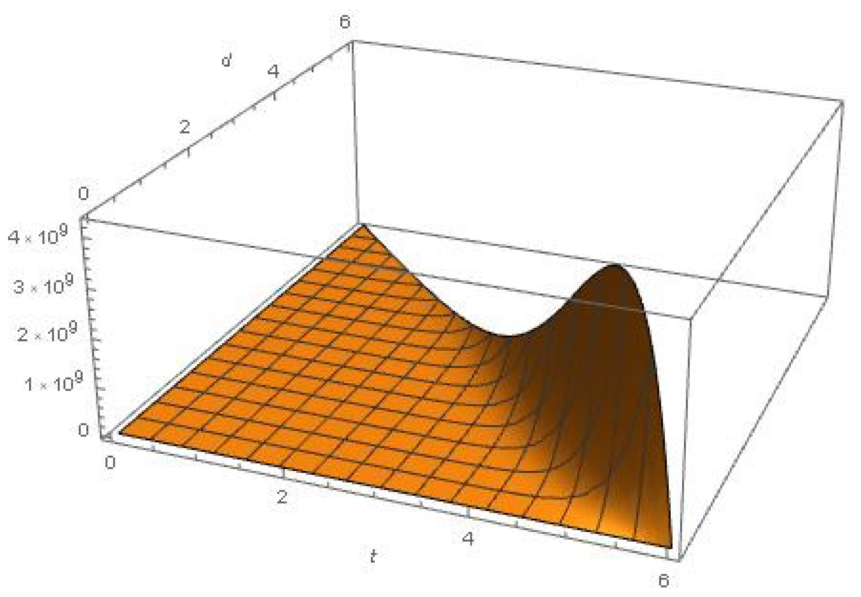Thus, an initial value will be needed just for this last one. Again, the cases of two and three observations will be studied:

  ○

  $n=2\Rightarrow \xi =\left\{t,t+d\right\}$. The determinant of the information matrix is

  $$\det \left(M_0\right)=\frac{{\beta }_0^2{d}^2{e}^{2\left({\beta }_1+1\right)d+4{\beta }_{1}t}}{e^{2d}-1},$$

  and it is clear that the values $t$ and $d$ maximizing this determinant will not depend on ${\beta }_0$. Figure 1 shows the determinant of the information matrix after removing ${\beta }_0^2$ and using the nominal value ${\beta }_{10}=1$ for the non-linear parameter. For primary school levels ($t_{max}=6$) and assuming a minimum distance $d_0=1$ between tests, the recommended design uses $t=5$ and $d=1$, that is, making the tests the last two years.

  ○

  $n=3\Rightarrow \xi =\left\{t,t+d_1,t+d_1+d_2\right\}$. The determinant of $M_0$ is

  $$\begin{array}{rrr}\hfill \det \left(M_0\right)& \hfill =& \hfill \frac{{\beta }_0^2{e}^{2\left({\beta }_1+1\right)d_1+d_2+4{\beta }_{1}t}}{\left(e^{d_1+d_2}-1\right)\left(e^{d_1}-2e^{d_2}+e^{2d_1+d_2}\right)}\\ \hfill & \hfill & \hfill [e^{d_2}{d}_1^2\left(-2e^{{\beta }_1{d}_2}+e^{2{\beta }_1{d}_2+d_1}+e^{d_1}\right)\\ \hfill & \hfill & \hfill -2d_2{d}_1{e}^{{\beta }_1{d}_2}\left(-e^{{\beta }_1{d}_1}-e^{\left({\beta }_1+1\right)d_2+d_1}+e^{{\beta }_1{d}_1+\left({\beta }_1+1\right)d_2}+e^{d_2}\right)\\ \hfill & \hfill & \hfill +d_2^2{e}^{\left(2{\beta }_1+1\right)d_2}\left(-2e^{{\beta }_1{d}_1}+e^{\left(2{\beta }_1+1\right)d_1}+e^{d_1}\right)],\end{array}$$

  and when removing β₀² and assuming t_max = 6 and d₀ = 1, the maximum for β₁₀ = 1 is attained when t = 4, d₁ = 1, and d₂ = 1, that is, testing the students the last three courses.

4. Discussion

In the last few years, there has seen a remarkable increase in the relevance of the design of experiments in social science areas [22]. Major issues in the education research area must be treated on a sequential multiscale temporal level. Educational policies such as curricula, reduction in class size, programs for students’ support, etc. are developed considering educational theories based on solid experimentation [23]. In addition, large-scale experiments may be unattainable, and some authors alert about extracting generalized conclusions from experiments in education [24]. There is a general agreement in trying to “maximize the scientific benefit using the resources available for an investigation” [25]; thus, the optimal design of experiments becomes a key piece on the research process.

Randomized experiments with multilevel implications have been used by educational researchers in order to determine the effect of some treatment through time. One of the most used techniques in this line is the sequential multiple assignment randomized trials (SMART) [23,26,27]. This approach gives information about the effectiveness of some intervention or treatment through time, but it does not discriminate factor variables [25,28]. As an alternative, factorial designs, with the feature of determining the influence of factors, have also been applied for similar purposes [25,29]. These factorial designs have been used as well to provide a relation between four different mathematical problem representations and the problem solving abilities of elementary school students from grades 1 to 3 [30]. Nevertheless, some limitations regarding to the independence of the variables, the quantity of considered factors, or the presence of more than two levels by factor are addressed [25]. Most of these studies assume independent observations; few consider some kind of relation between samples (for example, the intraclass-correlation between observations within a cluster in [25,31], but not complex correlation structures like the ones derived from the consideration of multiresponse models such as the ones studied in this work.

In educational research, observations are rarely independent, as pointed out in [32]. Mixed-effect regression models cover this and other issues, such as correlated data organized in a multilevel or hierarchical structure, missing data, variability, etc. [33,34,35]. Applications of these models in educational projects can be found in [32] where the correlation between the results of two tests taken before and after a treatment is studied, controlled for a variable with three levels. The levels correspond to three selected difficult topics to study, and a selection model based on AIC criterion is applied to conclude. In [36], mixed linear regression analysis is applied to a large database to establish the correlation between the student’s relationship and their academic performance. Finally, ref. [37] evaluated the impact of sequences of parents’ input on children’s language outcomes. Although all these applications are longitudinal or level studies, they are focused on selecting the best model for prediction, but no one addresses the issue of optimizing data recollection along time.

Despite being less known in the education area, generalized estimating equations (GEEs) are introduced in [38] as an alternative for the analysis of cross sectional clustered data with repeated measurements along time [39,40,41]. It shows GEEs as a generalization of linear general models and that its performance is similar to multilevel models (random effects or mixed model) and ordinary least squares. However, some limitations have to be considered, for example the impossibility of applying classical selection model techniques based on likelihood estimation, the lack of non-random data, and the amount of missing data. In addition, the number of clusters should be relatively high, and the observations in different clusters must be independent, although within-cluster observations may be correlated, as it is refereed in [40].

Again, it is necessary to highlight that none of these approaches seem to be fully appropriate to conduct experiments involving multiresponse and multisubject models with repeated observations in time, with potential correlation structures as the ones described in this paper. The novel approach presented here seems the most convenient for studies that could be similar to the one described in the example.

The relation between the variables ’Mental Representation’ and ’Mathematical Problem Resolution’ in primary school students was extensively studied in [3]. Now, the theory developed in Section 2 has been applied to that case for finding the best design (times when perform the tests to the students) in order to obtain an insight of the evolution of the two variables.

Assuming a sensible hypothesis about the correlation structure, two scenarios have been considered, one with different models of the variables for each subject and another one assuming the same model of each variable for every subject, obtaining interesting theoretical results especially in the second case. Two types of evolution models have been considered as well in order to stress that the optimal allocation of the tests may depend very much on the assumed model. The best design when assuming the linear regression model is making the tests near the extremes of the evaluation period. However, when the evolution is described by an exponential model, the results may be quite different since the optimal designs are very sensitive to the initial value of the parameters. The widely used exponential inter-correlation has been assumed. The preliminary study in [3] discovered that the group of the small (first year) students had a great variability, and thus it was not very informative. For this reason, when a design contains any temporal point belonging to the first school year (for instance when assuming a linear trend evolution), it will be convenient to delay these tests so that the analysis interval starts the second year of the primary school period.

A robustness study has been carried out for the exponential evolution model in order to check whether the optimal designs obtained are sensitive to the choice of the nominal value of ${\beta }_1$. It has been found that in fact the optimal designs can vary very much; for instance if $n=2$, the best designs found vary from the ones that take the extremes of the design interval when ${\beta }_{10}=0.1$ or the school years 4 and 6 when ${\beta }_{10}=0.5$ to those choosing the last temporal points when ${\beta }_{10}\ge 1$. A similar variability of results is obtained for $n=3$: when ${\beta }_{10}=0.1$, the proposal is to make one test at the beginning of the design interval and the other two at the end, and when ${\beta }_{10}=0.5$ assuming $d_0=1$, the most convenient school years to perform the tests are 3, 4, and 6.

Optimal designs have been computed for the $D$-optimality criterion, which is the most used, and two popular 2-parameter evolution models have been considered assuming always exponential inter-correlation. However, the procedure can be immediately extended to other optimality criteria, evolution models, and correlation kernels, provided that these can be assumed similar for all the variables.

5. Conclusions

The need to study the problem solving ability of primary school students, its relation with other variables, and the evolution of all of them was the inspiration of this work, from a previous study of [3]. In order to choose the best temporal points where samples should be taken to maximize the information of the collected data, a general procedure for several variables and subjects has been developed from the point of view of optimal design of experiments theory.

It should be noted that the results obtained in Section 2 are quite general and could be applied in other type of studies involving several subjects, with a $k>2$ number of variables of interest. Depending on the cost of every type of measure and the available budget, sometimes it might be convenient to select the variables that will be observed at a specific point instead of sampling all of them. The reason may be to save the cost of those measurements that are not considered so important or informative. Cost constraints could be incorporated into the model in a similar way as described in Chapter 5 of [42]. For instance, when two types of variables are to be observed, the problem can be stated as follows: two types of measurements $y_1$, $y_2$ can be made for every experimental unit, with costs $c_1$ and $c_2$, respectively. In the general case, every time that a subject is measured entails some cost $c$. For the total cost there are three possibilities:

• Measure $y_1$, with cost $c_1$. Total cost: $C_1=c+c_1$;
• Measure $y_2$, with cost $c_2$. Total cost: $C_2=c+c_2$;
• Measure both $y_1$ and $y_2$. Now the overall cost is $C_3=c+c_1+c_2$.

Possible scenarios are described by $t_x=\left\{t,x_1,x_2\right\}$, with $0\le t\le t_{max}$ and $x_1$, $x_2$ in $\left\{0, 1\right\}$ and $x_1+x_2>0$, where $x_i=1$ when test $y_i$ is made at a time $t$, and $x_i=0$ otherwise. The best designs fitting this budget may be non-balanced. In this case, the covariance matrices could be obtained as described in Example 2 of [1]. Ref. [42] discusses a procedure for studying this issue, but only for one subject and considering intra-correlation and not inter-correlation between samples, which are assumed independent. When there are more subjects and the two types of correlation are non-trivial, the problem becomes far more complex to deal with.

For this study, it has been assumed that the evolution models were similar in the different variables. Should these models be different, the covariance and information matrices would be much more complex, as would the computation of the optimal designs. The assumptions of equal intracorrelation in all the design points and equal intercorrelation for all the variables are quite sensible. In case that any of them (or both) were not true, the covariance matrices could not be expressed by Kronecker products, and the optimal designs for the global model would not be the same as the ones for the individual models of each variable for each subject; in fact, this global optimal design may be extremely difficult to compute.