
Resolution of Initial Value Problems of Ordinary Differential Equations Systems


Abstract
:1. Introduction
2. Numerical Analysis Tools
- (1)
- Working with computers that use finite precision mathematics, the first question to keep in mind is that in computational models, you have to try to avoid, whenever possible, the subtraction of functions that can have values of the same order. Such a subtraction produces a smaller result than that of the operands and it can lead to the loss of the most significant digits of the given value and produce the named catastrophic cancellation; see [48] (chapter 1). This operation is especially disastrous in numerical derivation processes as well as in recursive algorithms which are quite fashionable for their beauty and the simplicity of their implementation, as checked in the Ref. [48] (problem 2, chapter 1). It is also dangerous when a derivative (total or partial) is expected to change signs (detection of extremals in the corresponding function) because if it changes signs, it means that it has had to reach zero and lost all its significant digits. Therefore, we must always look for alternative formulas to those that appear in books and manuals (see Appendix B for the IEEE standards) for floating point computation, for intrinsic functions of programming languages, and for numerical derivatives.
- (2)
- The next step is to try to base our model on another with an analytical solution that is the limit of ours when a certain parameter tends to zero, for example (asymptotic model). If the asymptotic model has an analytical solution that provides us with certain AE to obtain values of some variables near those of our model, such values eventually serve to rescale or renormalize the variables of our model. This technique is very common in the N-body processes of physics (renormalization of sources), and even in the numerical solution of hyperbolic ODE and PDE which requires reconstruction of the axes at each step to avoid distortions if the coefficients vary with time.
- (3)
- At this point we need to verify that the functions we are going to use are evaluable with a precision greater than the tolerance we impose (standard IEEE). This analysis shows to what extent it is feasible to solve our model and which problems require modifications of the integrating algorithm.
- (4)
- A very important tool in simulations is to make variable changes, such as passing an affine parameter to the t variable that focuses more on knowing how much we have advanced and how much we still have to. We can also rely on the easy asymptotic solution to be calculated in order to define new variables that are quotients of the same variable in each system. These ratios have a very small range of variation, and we reduce the impact of noise (local error) on the objective function. Sometimes it is even possible to decouple some ODEs, as in the case discussed in the present paper.
- (5)
- We enter the phase of incorporating our objective function into the dynamical system that we have modelled through its analytical derivation (if it is an AE) so that it can evolve with the global model. If the values that this function take are very small compared to those obtained from the integration from other ODEs, we have to rescale the estimated values of the relative errors of each ODE in each step to avoid situations where the big ones dominate the small ones.
- (6)
- The decisive step is to modify the integrating method so that it only takes into account the relative error of the principal variables for the purpose of re-evaluating the integration step.
- (7)
- Extremal detection is also very important in order to modify the step. Usually, some of these extremals (zeros of the derivatives) indicate the areas of greatest effect and should not be ignored. In our RKF45ng algorithm, we indicate a way to achieve this, which has given us very good results in the past, although it is probably very improvable.
- (8)
- Finally, any modification we introduce must be intensively tested. The most accurate test is to get the algorithm of our nonlinear dynamical system to obtain the values of the asymptotic system when we make the corresponding parameter zero (background test), at least within the precision of the machine used for the defined variables. If the final algorithm passes this test, we can be sure that it will pass any other reasonable test.
3. The Physical Problem to Solve
- (a)
- Friedmann-Lemaître-Robertson-Walker solution (FLRW) which represents a homogeneous and isotropic space-time (with constant energy density ). This is the background Universe.
- (b)
- Lemaître-Tolman-Bondi solution (LTB) which accounts for a Universe with a unique great perturbation (an excess or a defect of energy density over the mean) which is a pressureless spherically symmetric solution and which asymptotically tends to a FLRW metric (background). This is a parametric solution and requires numerical methods to determine the necessary functions in every space-time point. See ([44,49]).
- Build a suitable algorithm (we will name it CS) to numerically solve the parametric LTB metric with sufficient precision.
- Generate a second numerical algorithm (we will call it RKF45ng) that allows the integration of the null geodesics equations (or paths of free photons) in LTB with appropriate initial conditions.
- Compute the gravitational anisotropy.
- Design suitable controls and tests to check the consistency of the obtained values. In order to do that, the following data are considered:
- 4.1.
- If the LTB perturbation, while photons are crossing it, stays with small density contrasts it is admissible to make a first-order analytical approximation, both in the Einstein Equations and in the null geodesics. Then one can integrate this linear analytical approximation. A linear code has been built for such a case. This code supplies a method to compare with the case when .
- 4.2.
- If one integrates the null geodesics of LTB generated with a null perturbation (), one should obtain a FLRW Universe and, therefore, null values of the anisotropy. This is a good test to detect systematic errors and loss of precision. Moreover, it will be the main tool to guarantee that the RKFng is stable. (Background test).
4. Solutions of EE Used
4.1. LTB Solution of EE
4.2. FLRW Solution of EE
5. CS Algorithm
5.1. Initial Functions
- (i)
- Computation of R(M,t): From Equation (1) and the density profile, one hasThis equation has a unique positive solution of for each . Once M is known, it can be written in the following way:and it can be applied to any method of roots computation as the solution is unique and simple. As in the FLRW, one has , and can be taken as an initial value for the Newton method. It still has to be determined whether the error tolerance is admissible for R. Therefore, a method to obtain the radial coordinate associated to each shell is achieved with a prefixed relative error bound. That is, the profile is obtained.
- (ii)
- Computation of f(M): By taking in Equations (2) and (3), one has:If , one of these equations has a solution (see Figure 2), from which z is obtained through a roots calculus and, afterwards, with the same precision when numerically solved for an arbitrary M and its corresponding . If no equations have a solution, that means that in the shell, the following is accomplished:and then, (limiting shell).
5.2. The Other Functions at
- As is known at (initial profile), in the Equation (1), one can directly compute the valuewith the same relative error bound as R.
- Furthermore, once and are known, one can also obtainwith the same relative error bound. So as to know the sign of this derivative, one needs to know whether, at a later time, increases or decreases for the same shell. The advantage of this procedure is that the derivative value is precise and no significant digits are lost (see Appendix B).
- The other functions appearing in the Christoffel symbols such as , y need derivation numerical techniques (a ) of the known functions , and , although one cannot now guarantee a fixed relative error bound, as the catastrophic cancellation phenomenon can appear through the loss of significative digits with the subtraction of similar numbers. The logarithmic derivative is crucial here.
5.3. Functions for
6. Additional Utility of the CS Algorithm
- Choose an and, together with the critical density value , determine for the asymptotic FLRW.
- With the core “radius” , choose (application of the scale factor). Additionally choose a value of the contrast for and compute the value of the FLRW.
- Simplify the CS algorithm to obtain only the and values. Apply it only at and for a predetermined sample of shells and obtain and .
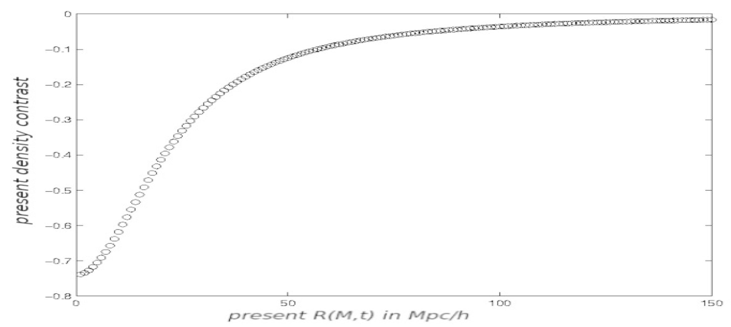
- Compute by extrapolation and (maximum present density contrast).
- Additionally compute or the present core radius by interpolation, first searching the value of the core shell, , such that and the corresponding value of .
- In this way, a function of two variables has been defined:evaluable for each pair of initial data.
- Now the numerical secant method for systems of equations allows to perform iterations, starting with two initial values y , until it is able to find the desired present maximum contrast and core radius (in the case where it converges, of course).
7. Resolution of the Null Geodesics EDOS
7.1. Numerical Instability of the Initial System
7.2. First Numerically Stable System
7.3. Inclusion of the Objective Function
7.4. Rescaling of the Variables. RKF45ng Algorithm
7.5. Convergence and Stability. FLRW Test for RKF45ng with
7.6. Convergence and Stability. New Tests for the RKF45ng When
7.6.1. Double-Integration Test
- ,
- ,
7.6.2. Direction Test
7.6.3. Extrapolation Test
7.6.4. Linear Test
- With both codes, linear and , the present temperature contrast is computed for values of . In the result is obtained by extrapolation. This way, the values of are known in 181 evenly spaced points.
- By taking into account that , the temperatures in each direction and their mean are computed:
- Now the new contrast is computed:As a consequence of this definition, the monopole of is null.
- The dipolar contribution to is related with the Observer–Symmetry Centre relative velocity (Doppler Effect). The other contributions to are named or nondipolar anisotropy contribution, and are computed by subtracting the dipolar part from .
- Given any inhomogeneity – of Table 1b, plots of the linear solution and of the solution are indistinguishable.
- For the case , the plots are shown in Figure 6a. The continuous plot corresponds to the linear computations, while the discontinuous plot corresponds to the non-linear ones ( algorithm). The figure shows that both results are very similar. This means there is very simultaneous effectiveness in both schemes. For the other inhomogeneities of Table 1b, we also obtained very similar results for both algorithms (linear and non-linear). Figure 6b plots the non-linear computations of for the cases – of Table 1b. In Figure 6b, we can appreciate that the CMB anistropy grows as the values of decrease. Therefore, these kinds of CMB anisotropies, values, are greater as the model of universe is more open.
8. Results and Discussion
9. Summary and Conclusions
Author Contributions
Funding
Institutional Review Board Statement
Informed Consent Statement
Data Availability Statement
Acknowledgments
Conflicts of Interest
Appendix A. Some Important Definitions
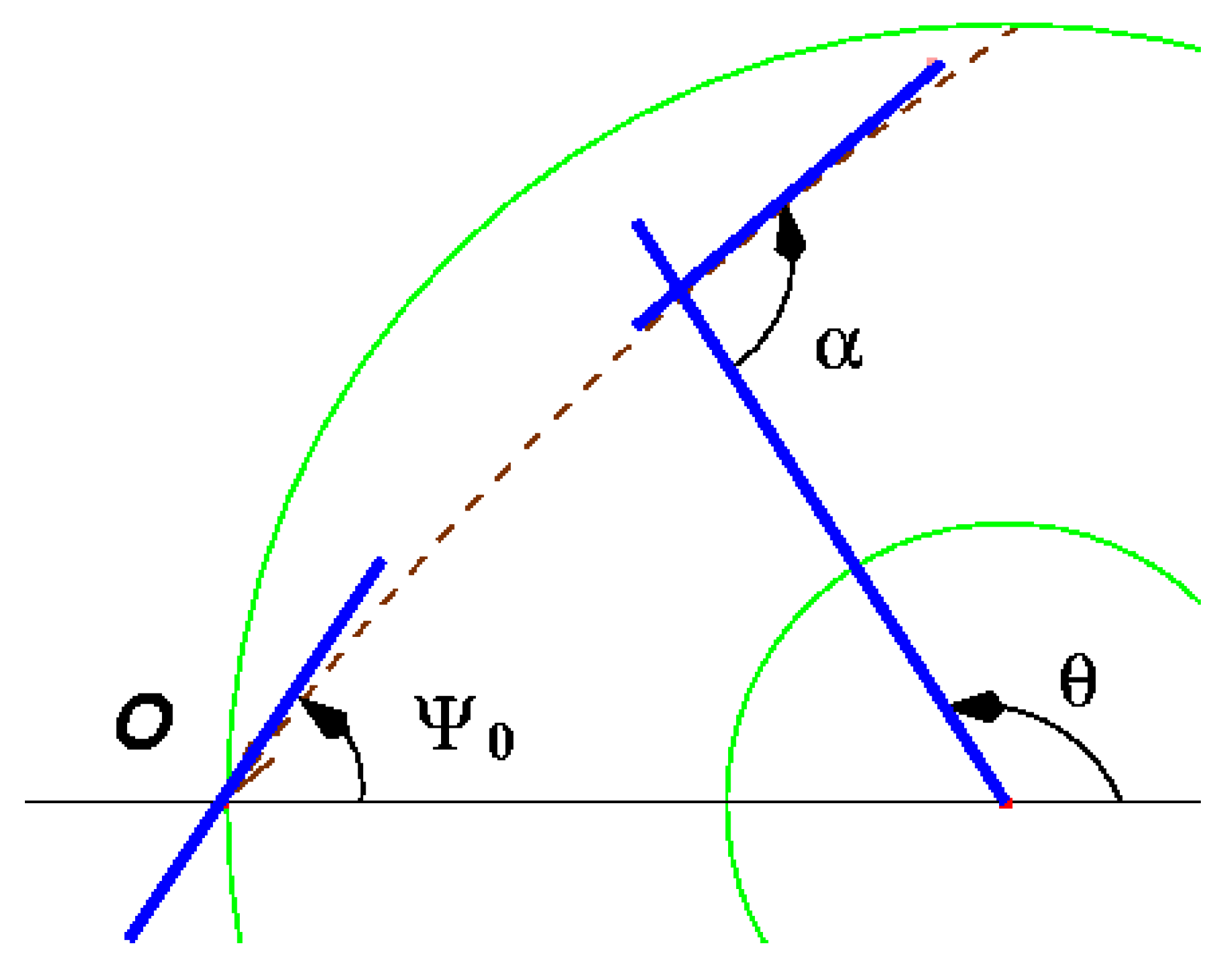
- Comoving coordinates. These coordinates assign constant spatial coordinate values to observers who measure the universe as isotropic. As such observers move along with the Hubble flow, they are called comoving observers. CMB is also perceived to be isotropic. It is useful, for our purposes, to assign comoving coordinates to every point of the universe because LFRW and LTB universes are in expansion. Moreover, due to the spherical symmetry of such universes we choose coordinates , with the origin in the symmetry centre of the perfect fluid which is their source. Furthermore, we take the coordinates (beeing O the observer), as the coordinate becomes useless in our study. Additionally, for symmetry reasons, it is sufficient to study the spatial half-plane that contains the axis (see Figure 1).The M coordinate is a label associated to every spatial spherical surface with centre in , named shell, and is related to the mass-energy contained in the surface defined by the shell. The radial coordinate of such a shell depends on the time and is related with M and through the EE.In FLRW, we choose an arbitrary point as the origin of coordinates and an arbitrary direction as the axis (at constant t, all the axes are equivalent) and the coordinates are also defined, where r is a radial coordinate, which is also comoving. The shells in this universe are a mere auxiliar definition which depends on the origin of coordinates.
- Decoupling time. This is defined as the time , where it can be considered that the dominant effect over the free photons is gravitational. This moment is as far as it is measured by the spectral lines Redshift . Decoupling time should be taken at . From this moment, photons freely propagate in the gravitational field of the Universe and its structures. As we are interested in computing the gravitational effect produced by nonlinear structures, we can take initial values at some suitable . In our work, we take initial values at Mpc (1 Mpc ≈ 3.2 lightyear).
- Scale factor. This is the time function included in the FLRW metric. The distances among galaxies are proportional to the scale factor and the following relation stands , where is the present time and Z is the redshift at time t.
- Critical density This is the mass density value such that, when it exceeds, the effect of gravity in the universe is great enough to stop its expansion in finite time. In our work, we used it to define different values of as background FLRW universes for our model of LTB. This definition is made through the density parameter . Thus, values such that originate FLRW open universes, while values originate closed FLRW universes. The case corresponds to a flat FLRW.
- Density profile. This is an initial condition to determine the LTB metric. At the initial time we take, in this work, a density profile given by:where gives the maximum density contrast and indicates the radial coordinate at which this contrast is reduced to a half (we call it core). As t varies, changes. The new profile in t may change its shape if the perturbation is nonlinear. Nevertheless, with linear perturbations it is acceptable that the shape of the profile remains the same.Both and besides , are initial values, for the searched algorithm. have been taken in the present work. With this initial profile, the spherical symmetry is guaranteed and the asymptotic FLRW limit with
Appendix B. Numerical Aspects to Take into Account
Appendix B.1. IEEE Norm

| Type | Long | Mantissa | Expo | Rounding Unit | Rank |
|---|---|---|---|---|---|
| Float | 32 bits | 24 bits | 8 bits | ||
| Double | 64 bits | 53 bits | 11 bits | ||
| Quad | 128 bits | 113 bits | 15 bits |
Appendix B.2. Intrinsic Functions
Appendix B.3. Numerical Derivation
References
- Perrin, C.L. Numerical Recipes in Fortran 90: The Art of Scientific Computing, Volume 2 (3 CD-ROMs and Manual); Press, W.H., Teukolsky, S.A., Vetterling, W.T., Flannery, B.P., Eds.; Cambridge University Press: New York, NY, USA, 1997. [Google Scholar]
- Butcher, J.C. A history of runge-kutta methods. Appl. Numer. Math. 1996, 20, 247–260. [Google Scholar] [CrossRef]
- Fehlberg, E. Low-Order Classical Runge-Kutta Formulas with Stepsize Control and Their Application to Some Heat Transfer Problems; National Aeronautics and Space Administration: Washington, DC, USA, 1969; Volume 315. [Google Scholar]
- Cash, J.R.; Karp, A.H. A variable order runge-kutta method for initial value problems with rapidly varying right-hand sides. ACM Trans. Math. Softw. TOMS 1990, 16, 201–222. [Google Scholar] [CrossRef]
- Lynch, S. Dynamical Systems with Applications Using MapleTM; Springer Science & Business Media: Berlin/Heidelberg, Germany, 2009. [Google Scholar]
- Lynch, S. Dynamical Systems with Applications Using MATLAB®; Springer: Berlin/Heidelberg, Germany, 2014. [Google Scholar]
- Lynch, S. Dynamical Systems with Applications Using Mathematica®; Springer: Berlin/Heidelberg, Germany, 2017. [Google Scholar]
- Lynch, S. Dynamical Systems with Applications Using Python; Springer: Berlin/Heidelberg, Germany, 2018. [Google Scholar]
- Zhu, Q. Stabilization of stochastic nonlinear delay systems with exogenous disturbances and the event-triggered feedback control. IEEE Trans. Autom. Control 2018, 64, 3764–3771. [Google Scholar] [CrossRef]
- Wang, H.; Zhu, Q. Global stabilization of a class of stochastic nonlinear time-delay systems with siss inverse dynamics. IEEE Trans. Autom. Control 2020, 65, 4448–4455. [Google Scholar] [CrossRef]
- Arnau, J.V.; Fullana, M.J.; Monreal, L.; Sáez, D. On the microwave background anisotropies produced by nonlinear voids. Astrophys. J. 1993, 402, 359–368. [Google Scholar] [CrossRef]
- Sáez, D.; Arnau, J.V.; Fullana, M.J. The imprints of the great attractor and the virgo cluster on the microwave background. Mon. Not. R. Astron. Soc. 1993, 263, 681–686. [Google Scholar] [CrossRef] [Green Version]
- Arnau, J.V.; Fullana, M.J.; Sáez, D. Great attractor-like structures and large-scale anisotropy. Mon. Not. R. Astron. Soc. 1994, 268, L17–L21. [Google Scholar] [CrossRef] [Green Version]
- Fullana, M.J.; Sáez, D.; Arnau, J.V. On the microwave background anisotropy produced by great attractor-like structures. Astrophys. J. Suppl. Ser. 1994, 94, 1–16. [Google Scholar] [CrossRef]
- Sáez, D.; Amau, J.V.; Fullana, M.J. Effects of great attractor-like objects on the cosmic microwave background. Astrophys. Lett. Commun. 1995, 32, 75. [Google Scholar]
- Fullana, M.J.; Arnau, J.V.; Sáez, D. On the microwave background anisotropy produced by big voids in open universes. Mon. Not. R. Astron. Soc. 1996, 280, 1181–1189. [Google Scholar] [CrossRef] [Green Version]
- Fullana i Alfonso, M.J. Anisotropies de la Radiació de fons de Microones Produïdes per Inhomogeneïtats Cosmològiques No Lineals; Servei de Publicacions de la Universitat de València: València, Spain, 1996. [Google Scholar]
- Fullana, M.J.; Arnau, J.V.; Sáez, D. Looking for the imprints of nonlinear structures on the cosmic microwave background. Vistas Astron. 1997, 41, 467–492. [Google Scholar] [CrossRef]
- Tsoulos, I.G.; Kosmas, O.T.; Stavrou, V.N. Diracsolver: A tool for solving the dirac equation. Comput. Phys. Commun. 2019, 236, 237–243. [Google Scholar] [CrossRef] [Green Version]
- Kosmas, T.S.; Lagaris, I.E. On the muon–nucleus integrals entering the neutrinoless μ–> e-conversion rates. J. Phys. G Nucl. Part. Phys. 2002, 28, 2907. [Google Scholar] [CrossRef] [Green Version]
- Kitano, R.; Koike, M.; Okada, Y. Detailed calculation of lepton flavor violating muon-electron conversion rate for various nuclei. Phys. Rev. D 2002, 66, 096002. [Google Scholar] [CrossRef] [Green Version]
- Stoica, S.; Mirea, M. New calculations for phase space factors involved in double-β decay. Phys. Rev. C 2013, 88, 037303. [Google Scholar] [CrossRef] [Green Version]
- Stoica, S.; Mirea, M.; Niţescu, O.; Nabi, J.; Ishfaq, M. New phase space calculations for β-decay half-lives. Adv. High Energy Phys. 2016. [Google Scholar] [CrossRef] [Green Version]
- Carleo, G.; Troyer, M. Solving the quantum many-body problem with artificial neural networks. Science 2017, 355, 602–606. [Google Scholar] [CrossRef] [Green Version]
- Snyder, J.C.; Rupp, M.; Hansen, K.; Müller, K.; Burke, K. Finding density functionals with machine learning. Phys. Rev. Lett. 2012, 108, 253002. [Google Scholar] [CrossRef] [PubMed]
- Arsenault, L.; Lopez-Bezanilla, A.; Lilienfeld, O.A.v.; Millis, A.J. Machine learning for many-body physics: The case of the anderson impurity model. Phys. Rev. B 2014, 90, 155136. [Google Scholar] [CrossRef] [Green Version]
- Torlai, G.; Mazzola, G.; Carrasquilla, J.; Troyer, M.; Melko, R.; Carleo, G. Neural-network quantum state tomography. Nat. Phys. 2018, 14, 447–450. [Google Scholar] [CrossRef] [Green Version]
- Engquist, B.; Fokas, A.; Hairer, E.; Iserles, A. Highly Oscillatory Problems; Cambridge University Press: Cambridge, UK, 2009; p. 366. [Google Scholar]
- Wendlandt, J.M.; Marsden, J.E. Mechanical integrators derived from a discrete variational principle. Phys. D Nonlinear Phenom. 1997, 106, 223–246. [Google Scholar] [CrossRef] [Green Version]
- Kane, C.; Marsden, J.E.; Ortiz, M. Symplectic-energy-momentum preserving variational integrators. J. Math. Phys. 1999, 40, 335–337. [Google Scholar] [CrossRef] [Green Version]
- Marsden, J.E.; West, M. Discrete mechanics and variational integrators. Acta Numer. 2001, 10, 357–514. [Google Scholar] [CrossRef] [Green Version]
- Hairer, E.; Lubich, C.; Wanner, G. Geometric numerical integration illustrated by the störmer–verlet method. Acta Numer. 2003, 12, 399–450. [Google Scholar] [CrossRef] [Green Version]
- Leimkuhler, B.; Reich, S. Simulating Hamiltonian Dynamics; Cambridge University Press: Cambridge, UK, 2004; Number 14. [Google Scholar]
- Ober-Blöbaum, S. Galerkin variational integrators and modified symplectic runge–kutta methods. IMA J. Numer. Anal. 2017, 37, 375–406. [Google Scholar] [CrossRef]
- Ober-Blöbaum, S.; Saake, N. Construction and analysis of higher order galerkin variational integrators. Adv. Comput. Math. 2015, 41, 955–986. [Google Scholar] [CrossRef]
- Campos, C.M.; Junge, O.; Ober-Blöbaum, S. Higher order variational time discretization of optimal control problems. arXiv 2012, arXiv:1204.6171. [Google Scholar]
- Kosmas, O.; Leyendecker, S. Variational integrators for orbital problems using frequency estimation. Adv. Comput. Math. 2019, 45, 1–21. [Google Scholar] [CrossRef] [Green Version]
- Kosmas, O. Energy minimization scheme for split potential systems using exponential variational integrators. Appl. Mech. 2021, 2, 431–441. [Google Scholar] [CrossRef]
- Kosmas, O.; Leyendecker, S. Family of higher order exponential variational integrators for split potential systems. J. Phys. Conf. Ser. 2015, 574, 012002. [Google Scholar] [CrossRef]
- Romero, P.D.; Candela, V.F. Blind deconvolution models regularized by fractional powers of the laplacian. J. Math. Imaging Vis. 2008, 32, 181–191. [Google Scholar] [CrossRef]
- Abbas, M.I.; Ragusa, M.A. On the hybrid fractional differential equations with fractional proportional derivatives of a function with respect to a certain function. Symmetry 2021, 13, 264. [Google Scholar] [CrossRef]
- Treeby, B.E.; Cox, B.T. Modeling power law absorption and dispersion in viscoelastic solids using a split-field and the fractional laplacian. J. Acoust. Soc. Am. 2014, 136, 1499–1510. [Google Scholar] [CrossRef] [Green Version]
- Candela, V.; Falcó, A.; Romero, P.D. A general framework for a class of non-linear approximations with applications to image restoration. J. Comput. Appl. Math. 2018, 330, 982–994. [Google Scholar] [CrossRef]
- Lemaître, G. Expansion of the universe, the expanding universe. Mon. Not. R. Astron. Soc. 1931, 91, 490–501. [Google Scholar] [CrossRef] [Green Version]
- Fullana, M.J.; Arnau, J.V.; Thacker, R.J.; Couchman, H.M.P.; Sáez, D. Estimating small angular scale cosmic microwave background anisotropy with high-resolution n-body simulations: Weak lensing. Astrophys. J. 2010, 712, 367. [Google Scholar] [CrossRef]
- Fullana, M.J.; Arnau, J.V.; Thacker, R.J.; Couchman, H.M.P.; Sáez, D. On the estimation and detection of the rees–sciama effect. Mon. Not. R. Astron. Soc. 2016, 464, 3784–3795. [Google Scholar] [CrossRef] [Green Version]
- Colmenero, N.P.; Córdoba, J.V.A.; Fullana i Alfonso, M.J. Relativistic positioning: Including the influence of the gravitational action of the sun and the moon and the earth’s oblateness on galileo satellites. Astrophys. Space Sci. 2021, 366, 1–19. [Google Scholar]
- Amat, S.; Aràndiga, F.; Arnau, J.V.; Donat Beneito, R.M.; Mulet Mestre, P.; Peris Sancho, R. Aproximació Numèrica; Servei de Publicacions de la Universitat de València: València, Spain, 2002. [Google Scholar]
- Bondi, H. Spherically symmetrical models in general relativity. Mon. Not. R. Astron. Soc. 1947, 107, 410–425. [Google Scholar] [CrossRef] [Green Version]
- Bardeen, J.M. Gauge-invariant cosmological perturbations. Phys. Rev. D 1980, 22, 1882–1905. [Google Scholar] [CrossRef]
- Saez, D.; Arnau, J.V. On the Tolman Bondi solution of Einstein’s Equations. Numerical Applications. In Recent Developments in Gravitation; World Scientific Publishing Co Pte Ltd.: Singapore, 1990; p. 415. [Google Scholar]
- Fullana, M.J.; Saez, D.P.; Monreal, L.; Arnau, J.V. The great attractor and the anisotropy of the microwave background. In Recent Developments in Gravitation; World Scientific Publishing Co Pte Ltd.: Singapore, 1992; p. 131. [Google Scholar] [CrossRef]
- Fullana, M.J.; Arnau, J.V. The Boötes void and the Cosmic Microwave Background. In Inhomogeneous Cosmological Models; World Scientific Publishing Co Pte Ltd.: Singapore, 1995; p. 125. [Google Scholar]
- Fullana, M.J.; Saez, D.; Arnau, J.V. The imprints of great voids on the cosmic microwave background. In Relativistic Astrophysics and Cosmology; World Scientific Publishing Co Pte Ltd.: Singapore, 1997; p. 121. [Google Scholar]
- Saez, D.; Arnau, J.V. Accurate simulations of the microwave sky at small angular scales. In Microwave Background Anisotropies, Proceedings of the XVIth Moriond Astrophysics Meeting, Les Arcs, Savoie, France, 16–23 March 1996; Editions Frontières: Singapore, 1997; p. 245. [Google Scholar]
- Sáez, D.; Arnau, J.V. Learning from observations of the microwave background at small angular scales. Astrophys. J. 1997, 476, 1. [Google Scholar] [CrossRef] [Green Version]
- Antoniou, I.; Papadopoulos, D.; Perivolaropoulos, L. Spinning particle orbits around a black hole in an expanding background. Class. Quantum Gravity 2019, 36, 085002. [Google Scholar] [CrossRef] [Green Version]
- Myron, M. Neue mechanik materieller systemes. Acta Phys. Polon. 1937, 6, 163–2900. [Google Scholar]
- Fullana Alfonso, M.J.; Saez Milán, D.P.; Arnau, J.V.; Colmenero, N.P. Some improvements on relativistic positioning systems. Appl. Math. Nonlinear Sci. 2018, 3, 161–166. [Google Scholar] [CrossRef] [Green Version]
- Puchades, N.; Fullana, M.J.; Arnau, J.V.; Saez, D. On the rees–sciama effect: Maps and statistics. Mon. Not. R. Astron. Soc. 2006, 370, 1849–1858. [Google Scholar] [CrossRef] [Green Version]


| (a) Nonlinear Underdensities | ||
| Case | ||
| 0.2 | −1.10 × | |
| 0.3 | −8.42 × | |
| 0.4 | −7.00 × | |
| 0.5 | −6.09 × | |
| 0.6 | −5.45 × | |
| 0.7 | −4.97 × | |
| 0.8 | −4.60 × | |
| 0.9 | −4.30 × | |
| 0.95 | −4.18 × | |
| 0.999 | −4.06 × | |
| (b) Overdensities | ||
| Case | ||
| 0.2 | 5.985 × | |
| 0.3 | 4.496 × | |
| 0.4 | 3.700 × | |
| 0.5 | 3.200 × | |
| 0.6 | 2.870 × | |
| 0.7 | 2.550 × | |
| 0.8 | 2.400 × | |
Publisher’s Note: MDPI stays neutral with regard to jurisdictional claims in published maps and institutional affiliations. |
© 2022 by the authors. Licensee MDPI, Basel, Switzerland. This article is an open access article distributed under the terms and conditions of the Creative Commons Attribution (CC BY) license (https://creativecommons.org/licenses/by/4.0/).
Share and Cite
Arnau i Córdoba, J.V.; Fullana i Alfonso, M.J. Resolution of Initial Value Problems of Ordinary Differential Equations Systems. Mathematics 2022, 10, 593. https://doi.org/10.3390/math10040593
Arnau i Córdoba JV, Fullana i Alfonso MJ. Resolution of Initial Value Problems of Ordinary Differential Equations Systems. Mathematics. 2022; 10(4):593. https://doi.org/10.3390/math10040593
Chicago/Turabian StyleArnau i Córdoba, Josep Vicent, and Màrius Josep Fullana i Alfonso. 2022. "Resolution of Initial Value Problems of Ordinary Differential Equations Systems" Mathematics 10, no. 4: 593. https://doi.org/10.3390/math10040593