1. Introduction
Computed tomography (CT) is a commonly used nondestructive diagnostic imaging technology [
1,
2]. Reconstruction-algorithm-related technology has always been the research focus. From the perspective of applied mathematics, CT reconstruction is essentially an inverse problem of the Radon transform [
3]. Therefore, the properties of the Radon transform have always been the research topic in the CT reconstruction field [
4,
5,
6,
7]. Among all algorithms based on the inverse Radon transform, the filtered back projection (FBP) technique is a typical case [
8], which is convenient to implement. However, due to the divergence of the ideal ramp function, the FBP technique cannot be equivalent to the rigorous Radon inverse transform. An accurate and efficient inverse Radon transform method is essential to the theoretical research of CT reconstruction.
For discrete projection data, the performance of the CT projection-wise filter is an important factor that affects the CT image quality. Presently, the most commonly used filters in FBP are the R-L filter [
9] and S-L filter [
10]. The CT image reconstructed by the R-L filter has a clear contour and high spatial resolution, but the image is affected by an obvious Gibbs phenomenon [
11]. Compared with the R-L filter, the CT image reconstructed by the S-L filter has a lighter Gibbs phenomenon and less pixel value error, but the sharpness of the contour edge is lower. Additionally, the reconstructed image quality usually needs to be quantified by evaluating indexes [
12,
13]. On the other hand, not all filters can be obtained by the traditional design method, which is realized by the inverse Fourier transform after windowing the ramp function in the frequency domain [
14]. For that reason, scholars have also studied some filter designing methods, which have achieved remarkable results [
15,
16,
17,
18]. Recently, a class of neural network and deep learning-based filter optimizing methods have been proposed and shown some advantages of machine learning [
19,
20,
21]. However, most of the proposed methods are aimed at certain targets without widespread applicability. Filter optimizing methods based on machine learning can be used to obtain some local optimal solutions, but in most cases, they cannot be proved to be a global optimal solution. The supplement of a theoretical basis is necessary.
This article has three main modules related to filter construction: the SDBP technique, the computational model for filters, and the basic composition of filters. Among them, the SDBP technique contributes a new approach for inverse Radon transform; the computational model for filters reveals the relationship between filter function and convolution kernel of data preprocessing; the basic composition of filters shows the decomposition and essential elements of filters. Their corresponding theorems are proposed and proved in the order of logical recurrence.
As an extension of the inverse Radon transform in the form of Hilbert transform, this article introduces an inverse Radon transform formula in the form of second-order divided difference back projection (SDBP). Different from the FBP technique, the SDBP technique calculates the second-order divided difference instead of filtering during data preprocessing. Theoretically, the SDBP technique is an approach for accurate CT reconstruction for dense sampling.
On the SDBP technique, a generalized construction model for CT projection-wise filters is proposed. It begins with the discrete projection data being restored into a continuous function by convolution with kernel function. By applying the SDBP formula to the restored second-order difference projection function, the relationship between filter function and convolution kernel is revealed. As an application, a variety of filters can be acquired by applying different kernel functions to the proposed computational model. In particular, the R-L filter and S-L filter can be acquired, respectively, with sinc kernel and rectangular kernel. As an image evaluation index, the root mean square error (RMSE) is used to evaluate the reconstruction accuracy of different filters. The result shows that the delta filter has the minimum reconstruction error among the tested filters.
By further applying the filter construction model, it is proved that any kind of filter can be decomposed into basic filters. Through simulations of CT reconstruction for the Shepp–Logan phantom and the digital resolution chart, some characteristics of the basic filters are demonstrated, which provide guidance for the filter design using other techniques. This study provides sufficient theoretical basis for the analysis of filters and makes a foundation for filter optimizing methods.
2. Inverse Radon Transform with SDBP Technique
The SDBP technique is an approach for the inverse Radon transform. For the projection data of dense sets, the SDBP technique is a practicable way to achieve accurate analytical reconstruction of the target function. The SDBP technique also provides an approach for CT reconstruction with a discrete sinogram, even if the sampling is not equidistant.
2.1. Radon Transform
Each refers to a variable, and each refers to a function. Given a target real function , for , assume that satisfies the following conditions:
Hypothesis 1. is continuous;
The double integralextending over the whole plane, converges;
For any arbitrary pointon the plane, , where.
Definition 1. The Radon transform ofis a linear integral transform in the plane, which is defined aswhereis the distance of straight linefrom the origin;.
The Radon-transformed functions defined in Equation (1) and the original functions constitute a function space of bijections.
2.2. SDBP Technique
For and , given the Radon transform of the target function to be solved, assume that satisfies the following conditions:
Hypothesis 2. The integralconverges;
, whereofis the second-order difference operator with respect to variable, and more specifically The first-order partial derivativeis continuous, or only has removable discontinuities;
The second-order partial derivativeis continuous, or only has removable or jump discontinuities.
On the premise of the Radon transform meeting Hypothesis 2, the formula of the SDBP technique for the inverse Radon transform is shown as follows:
Theorem 1. For,,, and, If
, the integrand is equal to the mean value of second-order partial derivatives of
on both sides of the index position, as
Compared with the inverse Radon transform in the form of the Hilbert transform, the SDBP technique is operable, for it avoids the derivation process and the divergence of the Hilbert-transformed function at singularity. The SDBP technique is not same as the second-order differential operation of lambda tomography [
22]. Compared with FBP, SDBP is also quite different in the data processing of projection values. SDBP does not need to introduce a filter function. Its realization process can be summarized as the following three steps:
Calculation of the second-order divided difference of the projection function under a certain projection angle;
Linear integration of the second-order divided difference at the projection position of the target point, which is calculated in step 1;
Rotational integration of the linear integral value calculated in step 2, also known as the back projection progress.
Proof of Theorem 1. In order to facilitate the subsequent proofs, some properties of Fourier transform are introduced primarily. The rules of functional relations of Fourier transform are shown in
Appendix A, in which the rules cited in this article are represented by ‘Rule Number’.
For the target
, on the promise that
satisfies Hypothesis 1, then according to the properties of Fourier transform, there is
where
are the independent variables in frequency domain corresponding to
;
represents the imaginary unit;
is the 2D Fourier transform for independent variables
; and
is the inverse 2D Fourier transform for independent variables
. Replace variable
, and combined with the Jacobian determinant, there is
The orthogonal direction integral of the rectangular coordinate system is transformed into the rotation direction integral of the polar coordinate system. According to the central slice theorem [
23], there is
where
is the Fourier transform with respect to variable
. For
in Equation (3), there is
where
represents the sign function. According to Rule 6, there is
where
represents the Dirac delta function. Combined with the principle of parity invariance,
By the inverse Fourier transform, there is
where
is the inverse Fourier transform with respect to variable
in the frequency domain. According to Rule 5, there is
By substituting Equations (4) and (5) into Equation (3), and according to Rule 1 and Rule 7, the inverse Radon transform formula in the form of the Hilbert transform is obtained, as
where
is the Hilbert transform with respect to variable
.
In Equation (6), the derivative term in the Hilbert transform is sensitive to the minor errors in the projections, which is not conducive to accurate reconstruction. The Hilbert transform is defined using the Cauchy principal value (marked with
) as
On the basis that the anomalous integral in Equation (7) converges, the right side of Equation (7) can be transformed by the partial integration as
where
is a constant. To ensure the validity of the partial integration, the convergence of the integral on the right side of Equation (8) must be guaranteed, so there is
. Equation (6) is further equivalent to
Eliminate the singularity of the integrand in Equation (9), then replace variable . Equation (2) is obtained, which is the formula of SDBP technique. Theorem 1 is proved. □
3. Computational Model for Filter Expressions
On the basis of the SDBP technique, a filter construction method is proposed. Implemented in the spatial domain, the method reveals the relationship between the filter function and convolution kernel, which can be used to restore discrete sampling data into continuous functions by convolution.
3.1. Projection Data Preprocess
For the target , on the premise that the projection of at any angle is systematic sampling data, it is assumed that the known conditions are as follows:
Hypothesis 3. The sampling interval of the detector is,
;
The projection angles are discrete at equal intervals, andis the number of total projections;
Forand, the projection value is defined as
where.
In order to acquire the continuous second-order difference projection function at any angle whose domain is , the discrete projection signal should be converted into a continuous function. The continuous second-order difference projection function of is constructed by projection values , where is the normalized variable of as . The constructed is expressed as follows:
Definition 2. For,,, and,whererepresents the convolution kernel function, andofsatisfies the following conditions: Hypothesis 4. For,,
is piecewise continuous, and the integral;
,, and;
is differentiable at any;
The second-order derivativeis continuous in the deleted neighborhood of any, andconverges on both sides of any.
3.2. Conversion Relation between Convolution Kernels and Filter Functions
The reconstructed value
of
can be approximated by the following formula [
14]:
where
;
represents the floor function, which gives the largest integer no greater than the input real number;
is the expression of filter, which can be obtained by
as follows:
Theorem 2. For,, there isif, there is For any given kernel function, its corresponding filter is uniquely determined. On the other hand, the kernel function corresponding to any given is not unique.
Given the analytic function (not unique) of , which is of , where is the normalized variable of as , the corresponding convolution kernel of is as follows:
Theorem 3. For,, there is By applying the proposed computational model, a variety of new filters can be obtained by designing the interpolation functions. Conversely, according to Equation (14), the kernel functions corresponding to some commonly used filters are revealed. Therefore, the filter expression is closely related to the restoration process of the projection signal.
Proof of Theorem 2. For the discrete projections, according to the SDBP technique, the inverse transform can be approximately expressed as
Replace variable
, then replace the second-order difference with
in Equation (10). The estimation formula of reconstructed
can be acquired as
According to Equation (10), Equation (15) can be further transformed into
In light of the operational characteristics of discrete convolution, Equation (16) can be transformed into Equation (11) in which
By performing partial integral in Equation (17), there is
Additionally, if satisfies Hypothesis 4 and is not differentiable at countable discrete points, refers to the generalized derivative. Combined with the definition of the Hilbert transform, Equation (12) can be acquired. Since the sum of all the coefficients in Equation (16) is zero, Equation (13) holds. Theorem 2 is proved. □
Proof of Theorem 3. Inversely, if the analytic function
of
is given, then
satisfies Equation (17) as
By the Fourier transform and according to Rule 7, there is
For
, according to Rule 5, there is
By substituting Equation (19) into Equation (18), the following equation is acquired after performing the inverse Fourier transform as
In Equation (20), there is
By substituting Equation (22) into Equation (21), it can be deducted that
According to Rule 7 and combined with Equation (4), the following equation is acquired after performing the Fourier transform on both sides of Equation (23) as
By substituting Equation (24) into Equation (20), and combined with the definition of the Hilbert transform, Equation (14) can be acquired. Theorem 3 is proved. □
It can be clearly observed that there is a reciprocal relationship between filter function
and kernel function
, which can be realized by the Hilbert transform, shown as follows:
Based on the principles above, the mutual conversion between the filter function and kernel function can be realized. It shows the correlation between the filter expression and convolution kernel, which is not available in the frequency domain windowing method and the Riesz transform method [
24].
4. Illustration with Examples
To verify the validity of the proposed method for constructing filters, we apply some common kernels to the proposed model as examples, by which some known filters are derived. We also compare the reconstruction errors of different filters.
4.1. R-L Filter: Kernel
If
of
is the Whittaker–Shannon interpolation of
, then the convolution kernel is the normalized sinc function as
The derivative of the normalized sinc function is
According to Equation (12), there is
By Equation (13),
where
represents the Riemann zeta function, and
. Therefore, the filter corresponding to the normalized sinc kernel is
Equation (25) is the expression of the R-L filter [
9].
4.2. S-L Filter: Kernel
If
of
is the proximal interpolation of
, then the kernel function is the unit rectangular function, as
where
represents the unit rectangular function. The generalized derivative of unit rectangular function is
According to Equation (12), there is
Therefore, the filter corresponding to the unit rectangular kernel is
Equation (26) is the expression of the S-L filter [
10].
4.3. Delta Filter: Kernel
If
of
is the sampling function with each amplitude
, then the convolution kernel is the unit delta function, as
According to Equation (12), there is
Therefore, the filter corresponding to the unit delta kernel is
The expression of the delta filter shown in Equation (27) was firstly proposed by Yu-chuan Wei et al. [
25], and was introduced as a practical filter to approximate the ideal filter.
4.4. Imaging Tests
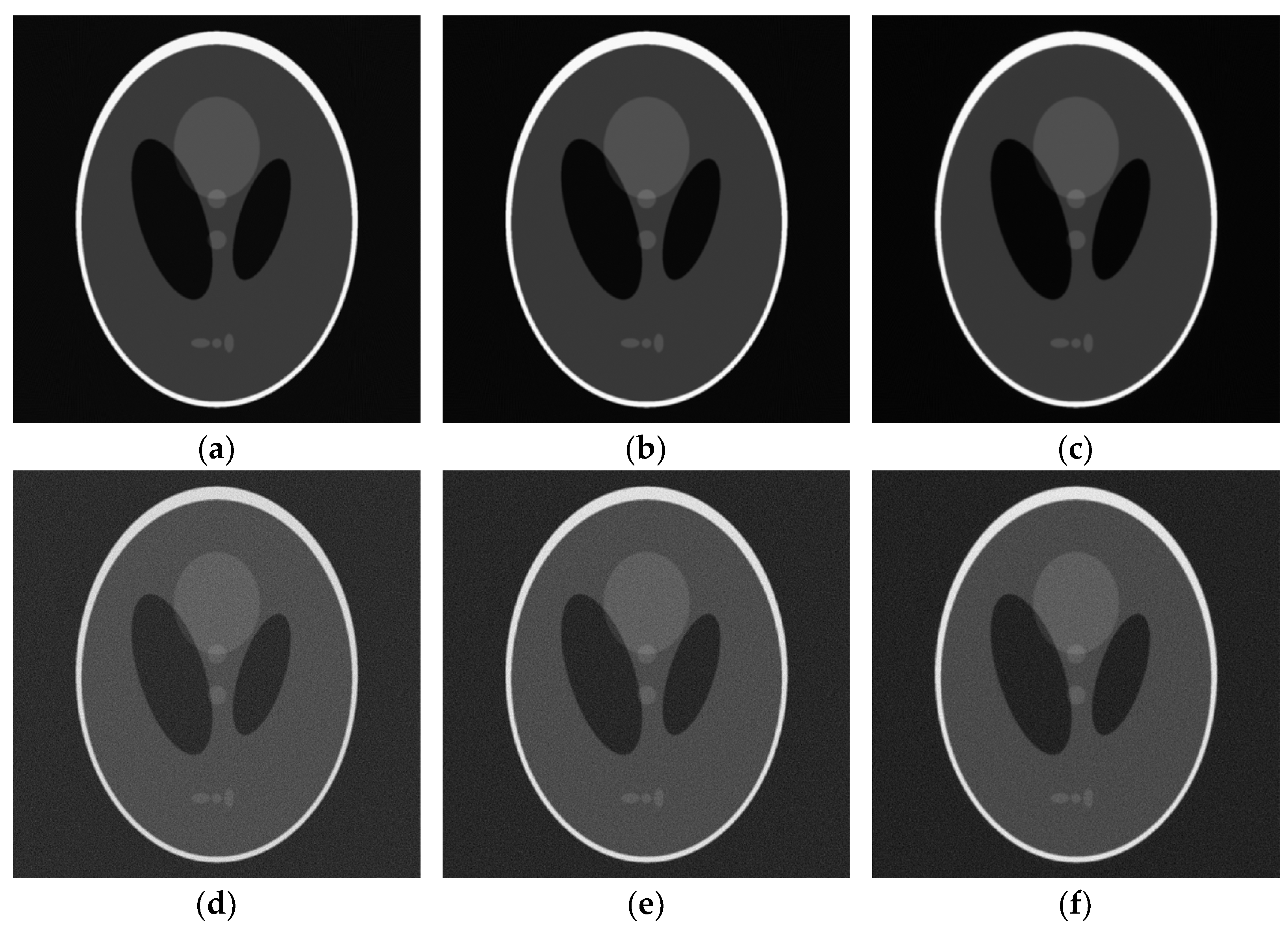
The Shepp–Logan phantom of 1024 × 1024 pixels was used to test the CT imaging performance of different example filters. The number of projections was set to 720, and the sampling interval of the detector was equal to the pixel size of the phantom. For further comparison, Gaussian white noise of standard deviation
was added to the sinogram to test the performance of the filters in noise. The reconstructed images are shown in
Figure 1.
To reflect the reconstruction accuracy more intuitively, we used the root mean square error (RMSE) to evaluate the error between the reconstructed image and the original image. The RMSE of CT image is defined as follows:
where
is the gray value of the original image pixel in row
and column
;
is the gray value of the reconstructed image pixel in row
and column
;
is the maximum value of
and column
. By calculation, the RMSE table of reconstructed images is shown in
Table 1, which shows that the reconstructed image of delta filter has the smallest RMSE under each noise intensity.
5. Analysis of Basic Composition of Filters
In order to make further explorations in the rules of the filter properties changing with the kernels, the basic components of filters are analyzed such that an arbitrary filter can be decomposed into a combination of basic filters, which is similar to the Fourier transform. The properties of basic filters provide guidance for the design of the kernel functions.
5.1. Decomposition of Kernel Functions
A generalized function can be described by Schwartz distribution. As for the kernel function
, its Schwartz distribution is defined by
where
represents the test function.
By performing discretization, the local function in a definite interval is regarded as a delta function whose amplitude is equal to the interval integral. In this way, the kernel function can be decomposed to a combination of delta functions. Assume that the interval between any adjacent integers is equally divided by piecewise intervals, then the discretized kernel function can be defined as follows:
Definition 3. For,, and,
Considering when
, by applying Equation (28) to Equation (29), there is
If
is continuous within its domain, according to the first mean value theorem for definite integrals, the discretized kernel
when
and the original kernel
have the identical Schwartz distribution,
To describe the basic elements of kernel functions, the delta_2 function is defined, which is described as follows:
Definition 4. For,,whererepresents the displacement of the delta functions from the origin. According to the conditions in Hypothesis 4,
can be expressed in the following form as
where
is the amplitude of delta_2 function,
According to Hypothesis 4, satisfies the following:
5.2. Filters of Basic Type
In the definition of Schwartz distribution, the delta_2 function is the basis function of any kernel. According to Equations (12) and (31), if
is the kernel function of
and
, there is
By Equation (13), the following equation can be acquired, as
The partial fraction decomposition of cotangent function can be used to calculate the exact value of
. For
, the sum of the sequence in Equation (34) is
Combined with Equation (33) and Equation (35), the filter expression corresponding to delta_2 function kernel is
Equation (36) is the expression of basic filter series. In particular, is the delta filter as .
A filter can be decomposed into a linear combination of basic filters, which is expressed as follows:
Theorem 4. For,, Proof of Theorem 4. The operation in Equation (12) is a special case of Schwartz distribution expressed in Equation (28). Combined with Equation (30), it can be concluded that
and
correspond to the same filter when
, which means
where
corresponds to
. On the basis of the linearity in Equation (12), it can be derived from Equation (32) that
If
is continuous for
, then
Suppose that
is continuous for
. According to Equations (38) and (39), there is
By means of the definition of integral, Equation (37) can be obtained by the conversion of Equation (40). Under the constraint of Hypothesis 4, it can be proved that Equation (37) is still valid in the case that the kernel function contains finite discontinuities, which include delta function components. Theorem 4 is proved. □
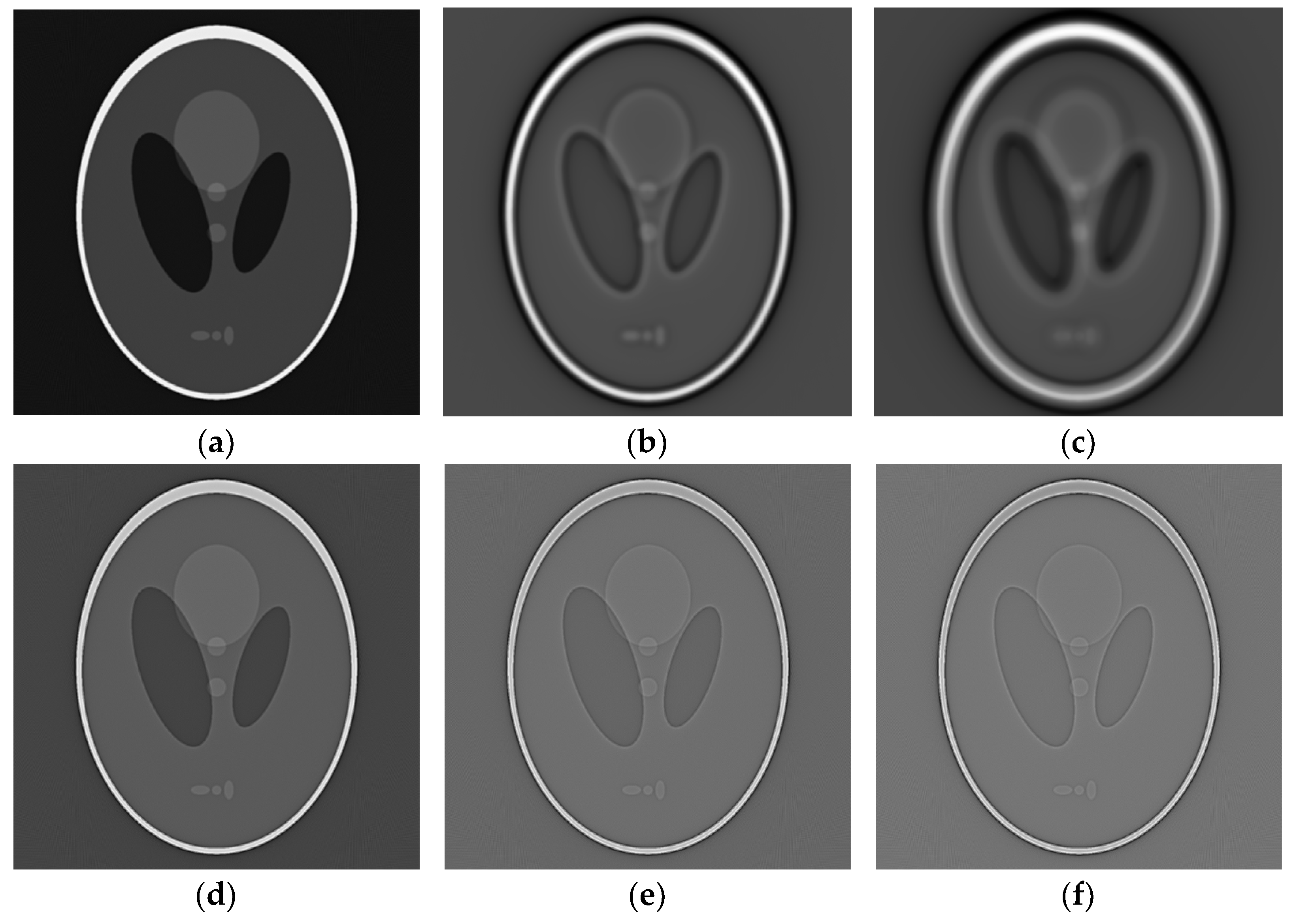
5.3. Imaging Tests
The Shepp–Logan phantom of 1024×1024 pixels was used to test the CT imaging performance of different basic filters. The number of projections was set to 720, and the sampling interval of the detector was equal to the pixel size of the phantom. The images of the Shepp–Logan phantom were reconstructed by a number of basic filters with different
, and some results are shown in
Figure 2.
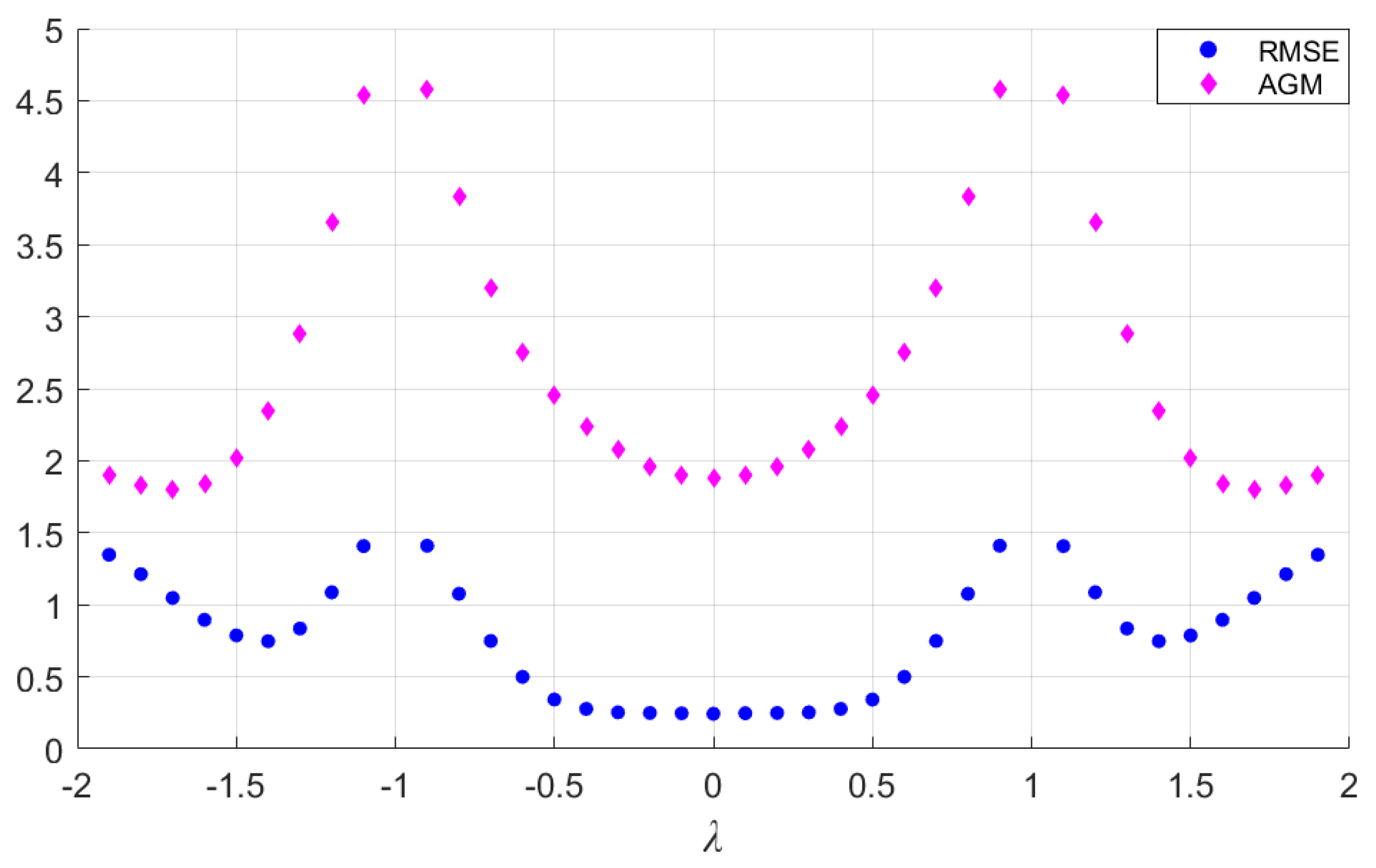
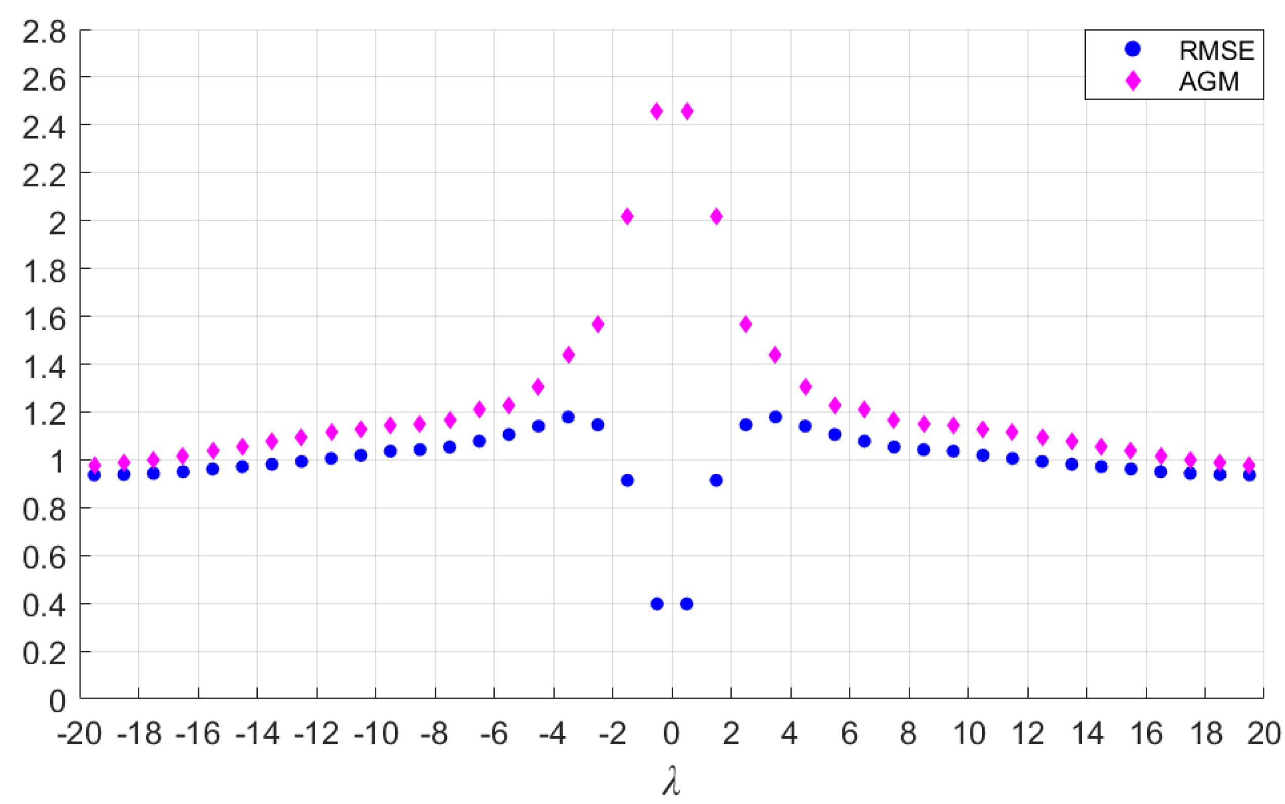
In addition to RMSE, we used the average gradient module (AGM) to measure the sharpness of the CT images. The image sharpness has a positive correlation with AGM. The computing formula of the CT image AGM is as follows:
The calculated RMSE and AGM of CT images reconstructed by basic filters are shown in
Figure 3 and
Figure 4, and the corresponding data set is provided in
Appendix B.
If the parameter
is divided into two parts, integer and decimal, as
(
and
), it can be summarized from
Figure 3 and
Figure 4 that the reconstructed image gradually blurs with the increase in
while
is constant, and the sharpness of the image increases as
is closer to 0 while
is constant. The RMSE is minimal only when
. The phenomenon verifies that the delta filter has the characteristic of minimal reconstruction error.
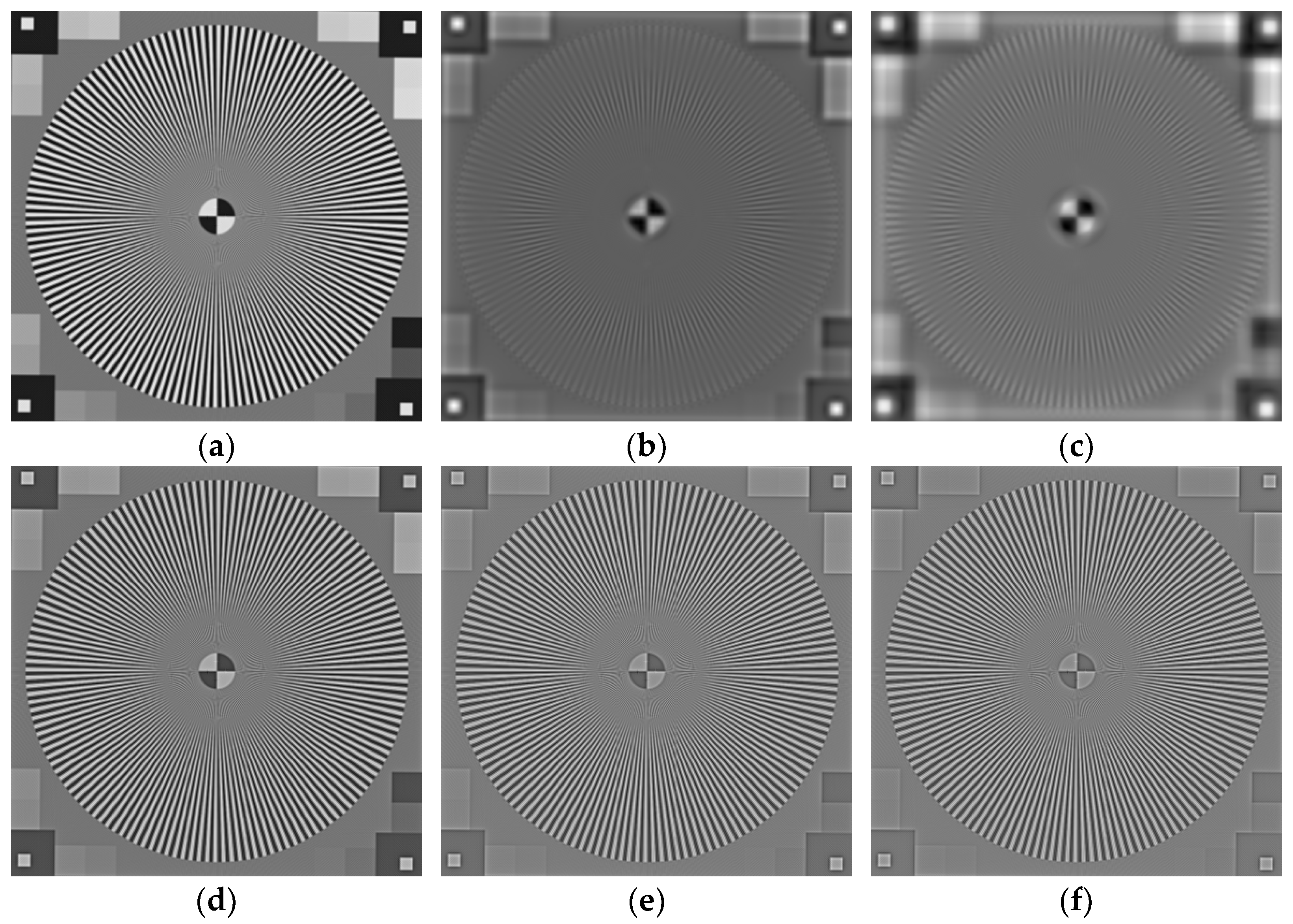
The simulated digital resolution chart of 1024 × 1024 pixels was reconstructed by basic filters with different
to highlight the phenomenon mentioned above. The number of projections was set to 1440, and the sampling interval of the detector was equal to the pixel size of the phantom. Some results are shown in
Figure 5.
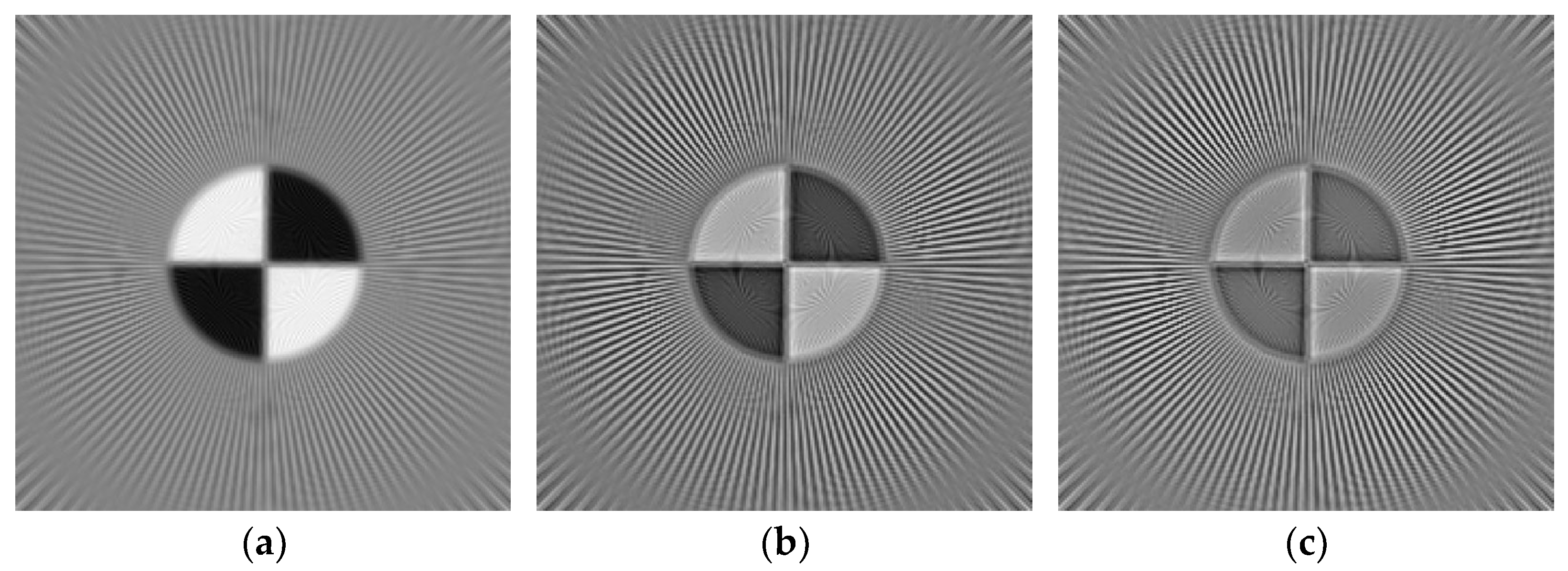
By observing the local centers of the reconstructed images shown in
Figure 6, it can be noticed that the stripes near center become clearer as
is closer to 0 while
is constant, indicating improved resolution.
6. Discussion
The convolution kernel mentioned in this article is basically used for projection data restoration. Meanwhile, the kernel is the inverse Fourier transform of the filtering window function in the frequency domain. In that sense, the proposed method indicates that the applicable window function has more possibilities, and even that the window function does not necessarily have to converge. It shows from a side view that the traditional filter design method does have some limitations.
As a conclusion, any CT image reconstructed through FBP is a linear superposition of the images reconstructed by basic filters. However, there are more properties of basic filters that need to be revealed. Additionally, the optimal composition of the basic filters remains a subject to be studied. This article mainly describes the relevant theories of filter construction, about the rationale extension and basic filter decomposition. The possible applications of the theories need to be further explored, which are not discussed here.
7. Conclusions
The SDBP technique proposed in this article is an approach for an accurate inverse Radon transform, which can be realized through a series of well-defined calculation processes. The transformation between the filter function and convolution kernel is derived from the SDBP formula. The conversion relationship indicates a systematic filter design method, showing that a desired filter can be acquired by an appropriate convolution kernel. By extension, a decomposition method of filters is proposed. For all filters used for CT reconstruction, any of them can be decomposed into basic filters. Some characteristics of the basic filters are demonstrated through simulations of CT reconstruction for the Shepp–Logan phantom and the digital resolution chart. By comparing RMSE and AGM, it is concluded that the error and resolution of the basic filter reconstructed image change periodically with parameter . As an inference, the properties of basic filters can be exploited to construct filters that meet some certain index requirements.
Author Contributions
Conceptualization, Y.J.; methodology, Y.J.; validation, Y.J. and J.Z. (Jing Zou); formal analysis, Y.J.; data curation, J.Z. (Jintao Zhao); writing—original draft preparation, Y.J.; writing—review and editing, J.Z. (Jing Zou) and J.Z. (Jintao Zhao); supervision, X.H.; project administration, X.H.; funding acquisition, J.Z. (Jing Zou) All authors have read and agreed to the published version of the manuscript.
Funding
This research was funded by the General Program of National Natural Science Foundation of China (grant number 61771328) and the National Key Research and Development Program of China (grant number 2017YFB1103900).
Institutional Review Board Statement
Not applicable.
Informed Consent Statement
Not applicable.
Data Availability Statement
Not applicable.
Conflicts of Interest
The authors declare no conflict of interest. The funders had no role in the design of the study; in the collection, analyses, or interpretation of data; in the writing of the manuscript; or in the decision to publish the results.
Appendix A
Table A1.
Table of some functional Fourier transform pairs [
26].
Table A1.
Table of some functional Fourier transform pairs [
26].
| Rule Number | Function | Fourier Transform |
|---|
| 0 | | |
| 1 | | |
| 2 | | |
| 3 | | |
| 4 | | |
| 5 | | |
| 6 | | |
| 7 | | |
| 8 | | |
Appendix B
Table A2.
Data set of RMSE and AGM of reconstructed Shepp–Logan images by basic filters with different .
Table A2.
Data set of RMSE and AGM of reconstructed Shepp–Logan images by basic filters with different .
| λ Value | RMSE | AGM |
|---|
| 0 | ±0.1 | 0.2824 | 0.2867 | 1.8782 | 1.9003 |
| ±0.2 | ±0.3 | 0.2890 | 0.2942 | 1.9617 | 2.0801 |
| ±0.4 | ±0.5 | 0.3221 | 0.3975 | 2.2354 | 2.4578 |
| ±0.6 | ±0.7 | 0.5801 | 0.8699 | 2.7555 | 3.1952 |
| ±0.8 | ±0.9 | 1.2499 | 1.6373 | 3.8340 | 4.5736 |
| ±1.1 | ±1.2 | 1.6345 | 1.2620 | 4.5341 | 3.6529 |
| ±1.3 | ±1.4 | 0.9700 | 0.8676 | 2.8780 | 2.3502 |
| ±1.5 | ±1.6 | 0.9142 | 1.0400 | 2.0154 | 1.8432 |
| ±1.7 | ±1.8 | 1.2166 | 1.4085 | 1.8012 | 1.8297 |
| ±1.9 | ±2.5 | 1.5649 | 1.1463 | 1.9009 | 1.5652 |
| ±3.5 | ±4.5 | 1.1787 | 1.1407 | 1.4371 | 1.3034 |
| ±5.5 | ±6.5 | 1.1055 | 1.0779 | 1.2284 | 1.2093 |
| ±7.5 | ±8.5 | 1.0533 | 1.0425 | 1.1680 | 1.1519 |
| ±9.5 | ±10.5 | 1.0359 | 1.0189 | 1.1417 | 1.1248 |
| ±11.5 | ±12.5 | 1.0056 | 0.9930 | 1.1149 | 1.0965 |
| ±13.5 | ±14.5 | 0.9813 | 0.9711 | 1.0747 | 1.0532 |
| ±15.5 | ±16.5 | 0.9614 | 0.9498 | 1.0377 | 1.0167 |
| ±17.5 | ±18.5 | 0.9431 | 0.9384 | 0.9981 | 0.9874 |
| ±19.5 | | 0.9365 | | 0.9754 | |
References
- Buynak, C.F.; Bossi, R.H. Applied X-ray computed tomography. Nucl. Instrum. Methods Phys. Res. Sect. B Beam Interact. Mater. Atoms. 1995, 99, 772–774. [Google Scholar] [CrossRef]
- Plessis, A.D.; Roux, S.; Guelpa, A. Comparison of medical and industrial X-ray computed tomography for non-destructive testing. Case Stud. Nondestruct. Test. Eval. 2016, 6, 17–25. [Google Scholar] [CrossRef] [Green Version]
- Radon, J. On the determination of functions from their integral values along certain manifolds. IEEE Trans. Med. Imaging 1986, 5, 170–176. [Google Scholar] [CrossRef] [PubMed]
- Park, H.S.; Lee, S.M.; Kim, H.P.; Seo, J.K.; Chung, Y.E. CT sinogram consistency learning for metal induced beam hardening correction. Med. Phys. 2018, 45, 5376–5384. [Google Scholar] [CrossRef] [PubMed] [Green Version]
- He, J.; Wang, Y.; Ma, J. Radon inversion via deep learning. IEEE Trans. Med. Imaging 2020, 39, 2076–2087. [Google Scholar] [CrossRef] [PubMed] [Green Version]
- Wang, L.C.; Zhang, C.H.; Zeng, Y.Z.; Yu, H.J.; Wang, Y. Application of Image Reconstruction Based on Inverse Radon Transform in CT System Parameter Calibration and Imaging. Complexity 2021, 2021, 5360716. [Google Scholar] [CrossRef]
- Huang, H.; Tang, W.; Yang, J.; Wang, L. Parameters Calibration of CT System Based on Geometric Model and Inverse Radon Transform. In Proceedings of the 10th International Conference on Applied Science, Engineering and Technology, Qingdao, China, 25–26 July 2021. [Google Scholar]
- Willemink, M.J.; Noël, P.B. The evolution of image reconstruction for CT—from filtered back projection to artificial intelligence. Eur. Radiol. 2019, 29, 2185–2195. [Google Scholar] [CrossRef] [PubMed] [Green Version]
- Ramachandran, G.N.; Lakshminarayanan, A.V. Three-dimensional Reconstruction from Radiographs and Electron Micrographs: Application of Convolutions instead of Fourier Transforms. Proc. Natl. Acad. Sci. USA 1971, 68, 2236–2240. [Google Scholar] [CrossRef] [PubMed] [Green Version]
- Shepp, L.A.; Logan, B.F. The Fourier reconstruction of a head section. IEEE Trans. Nucl. Sci. 2013, 21, 21–43. [Google Scholar] [CrossRef]
- Ramachandran, G.N.; Lakshminarayanan, A.V.; Kolaskara, A.S. Theory of the non-planar peptide unit. Biochim. Et Biophys. Acta (BBA)-Protein Struct. 1973, 303, 8–13. [Google Scholar] [CrossRef]
- Oyama, A.; Kumagai, S.; Arai, N.; Takata, T.; Saikawa, Y.; Shiraishi, K.; Kotoku, J.I. Image quality improvement in cone-beam CT using the super-resolution technique. J. Radiat. Res. 2018, 59, 501–510. [Google Scholar] [CrossRef] [PubMed]
- Kumar, M.; Aggarwal, J.; Rani, A.; Stephan, T.; Shankar, A.; Mirjalili, S. Secure video communication using firefly optimization and visual cryptography. Artif. Intell. Rev. 2021, 2021, 1–21. [Google Scholar] [CrossRef]
- Hsieh, J. Computed Tomography: Principles, Design, Artifacts, and Recent Advances; SPIE Press: Bellingham, WA, USA, 2003. [Google Scholar]
- Ludwig, J.; Mertelmeier, T.; Kunze, H.; Härer, W. A novel approach for filtered backprojection in tomosynthesis based on filter kernels determined by iterative reconstruction techniques. In Proceedings of the 9th International Workshop on Digital Mammography, Tucson, AZ, USA, 20–23 July 2008. [Google Scholar]
- Shi, H.; Luo, S. A novel scheme to design the filter for CT reconstruction using FBP algorithm. Biomed. Eng. Online 2013, 12, 50. [Google Scholar] [CrossRef] [PubMed] [Green Version]
- Lagerwerf, M.J.; Palenstijn, W.J.; Kohr, H.; Batenburg, K.J. Automated FDK-filter selection for Cone-beam CT in research environments. IEEE Trans. Comput. Imaging 2020, 6, 739–748. [Google Scholar] [CrossRef]
- Muders, J. Geometrical Calibration and Filter Optimization for Cone-Beam Computed Tomography. Ph.D. Thesis, Heidelberg University, Heidelberg, Germany, 2015. [Google Scholar]
- Syben, C.; Stimpel, B.; Breininger, K.; Würfl, T.; Fahrig, R.; Dörfler, A.; Maier, A. Precision Learning: Reconstruction Filter Kernel Discretization. arXiv 2017, arXiv:1710.06287. [Google Scholar]
- Ge, Y.; Zhang, Q.; Hu, Z.; Chen, J.; Shi, W.; Zheng, H.; Liang, D. Deconvolution-based backproject-filter (bpf) computed tomography image reconstruction method using deep learning technique. arXiv 2018, arXiv:1807.01833. [Google Scholar]
- Yamaev, A.; Chukalina, M.; Nikolaev, D.; Sheshkus, A.; Chulichkov, A. Lightweight denoising filtering neural network for FBP algorithm. In Proceedings of the 13th International Conference on Machine Vision, Rome, Italy, 2–6 November 2020. [Google Scholar]
- Quinto, E.T.; Skoglund, U.; Öktem, O. Electron lambda tomography. Proc. Natl. Acad. Sci. USA 2009, 106, 21842–21847. [Google Scholar] [CrossRef] [PubMed] [Green Version]
- Bracewell, R.N. Strip integration in radio astronomy. Aust. J. Phys. 1956, 9, 198–217. [Google Scholar] [CrossRef] [Green Version]
- Natterer, F. The Mathematics of Computerized Tomography; SIAM: Philadelphia, PA, USA, 2001. [Google Scholar]
- Wei, Y.; Wang, G.; Hsieh, J. An intuitive discussion on the ideal ramp filter in computed tomography. Comput. Math. Appl. 2005, 49, 731–740. [Google Scholar] [CrossRef] [Green Version]
- Kammler, D.W. A First Course in Fourier Analysis; Cambridge University Press: Cambridge, UK, 2007. [Google Scholar]
| Publisher’s Note: MDPI stays neutral with regard to jurisdictional claims in published maps and institutional affiliations. |
© 2022 by the authors. Licensee MDPI, Basel, Switzerland. This article is an open access article distributed under the terms and conditions of the Creative Commons Attribution (CC BY) license (https://creativecommons.org/licenses/by/4.0/).


