Article

Remaining Useful Life Estimation of Aircraft Engines Using Differentiable Architecture Search

1
School of Energy and Power Engineering, Beihang University, Beijing 100191, China
2
College of Electrical Engineering and Automation, Shandong University of Science and Technology, Qingdao 266590, China
3
School of Automation Science and Electrical Engineering, Beihang University, Beijing 100191, China
4
Institute of Artificial Intelligence, Beihang University, Beijing 100191, China
*
Author to whom correspondence should be addressed.
Mathematics 2022, 10(3), 352; https://doi.org/10.3390/math10030352
Submission received: 20 December 2021 / Revised: 12 January 2022 / Accepted: 20 January 2022 / Published: 24 January 2022
(This article belongs to the Topic Machine and Deep Learning)

Abstract

:
Prognostics and health management (PHM) applications can prevent engines from potential serious accidents by predicting the remaining useful life (RUL). Recently, data-driven methods have been widely used to solve RUL problems. The network architecture has a crucial impact on the experiential performance. However, most of the network architectures are designed manually based on human experience with a large cost of time. To address these challenges, we propose a neural architecture search (NAS) method based on gradient descent. In this study, we construct the search space with a directed acyclic graph (DAG), where a subgraph represents a network architecture. By using softmax relaxation, the search space becomes continuous and differentiable, then the gradient descent can be used for optimization. Moreover, a partial channel connection method is introduced to accelerate the searching efficiency. The experiment is conducted on C-MAPSS dataset. In the data processing step, a fault detection method is proposed based on the k-means algorithm, which drops large valueless data and promotes the estimation performance. The experimental result shows that our method achieves superior performance with the highest estimation accuracy compared with other popular studies.

1. Introduction

The prognostics and health management (PHM) of aircraft engines has received increasing attention owing to the fast development of deep learning. Remaining useful life (RUL) estimation, which is a technical term used to describe the progression of faults in PHM [1], is defined as the time from the current moment to the end of the useful life. In traditional industry, RUL estimation mainly depends on the physical model-based method. In the first international conference on prognostics and health management, Saxena et al. [2] used a damage propagation model to predict the RUL value. In comparison with other model-based methods (e.g., Arrhenius and Eyring models), Saxena achieved a better performance. Owing to the highly nonlinear features, it is difficult to improve the performance to a relatively large extent on physical model-based methods.
Apart from model-based methods, data-based methods have become more popular and are widely used in the industry. With the attribution of the fast development of neural networks (NN) [3], data-based methods have achieved great progress in RUL problems. Heimes proposed a method based on recurrent neural networks (RNN) [4], whereas Peel proposed a method using a Kalman filter based on NN [5], both of which have achieved excellent performance in the PHM08 conference. To date, convolutional neural networks (CNN) and RNN have become the most important branches of NN. Thus, great achievements have been realized in signal processing [6] and motion captures [7]. Several advanced networks have been proposed based on CNN and RNN (for instance, deep convolution neural networks (DCNN) [8,9], echo state networks [10], and long short-term memory networks (LSTM) [11]).
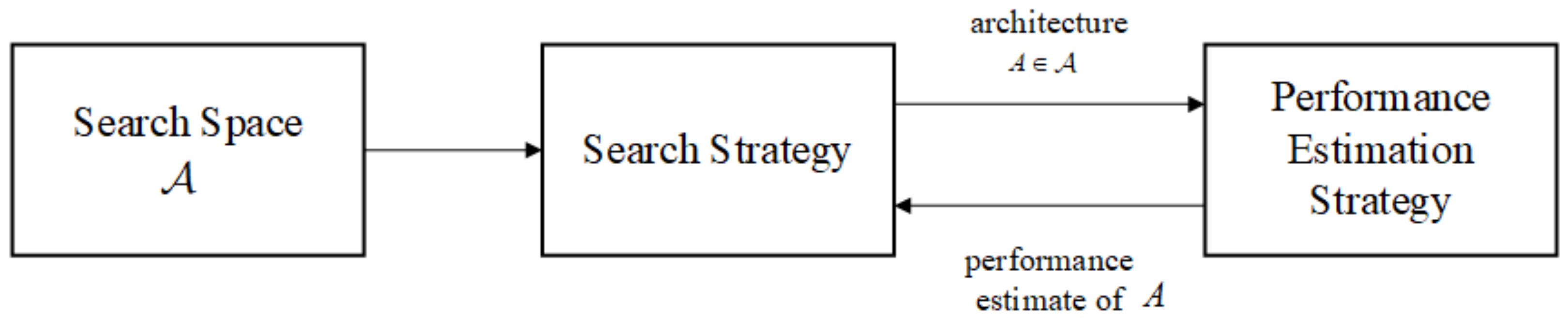
Compared with manually designed networks, whose performances are mainly dominated by the fixed network architecture and hyper parameters, neural architecture search (NAS) is a more efficient method to design a proper architecture [12]. The performance of NAS mainly depends on the transformative network architecture and NAS has achieved success in image classification and semantic segmentation [13,14]. According to different methods used in the architecture search, the search strategies can be divided into several categories: random search, reinforcement learning (RL), evolutionary algorithm, Bayesian optimization (BO), and gradient-based algorithm [15]. To solve the NAS problem in a RL method [16,17], the generation of a neural architecture can be considered to be the agent’s action, and the search space is considered the action space. The performance of the candidate architecture is identical to the agent’s reward. However, because of the reason that there is no external observed state and intermediate rewards, the RL method on NAS is more similar to a stateless multi-armed bandit problem. The first method of an evolutionary algorithms for network architecture dates back to the work of Miller at al. [18] in which the genetic algorithm is proposed to design architectures and backpropagation is used to optimize the weights. Since then, many works have used similar methods to optimize the network architecture weights [19,20,21]. Bayesian optimization on NAS was first proposed by Swersky et al. [22] and Kandasamy et al. [23]; in their works, kernel functions is derived for architecture search spaces in order to use classic GP-based BO methods.
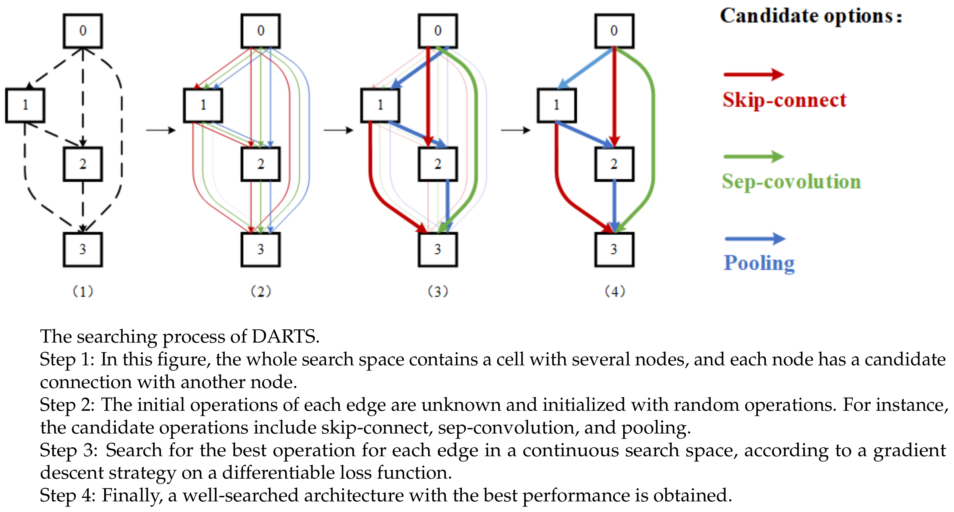
Different from these approaches, a softmax function is used to optimize the edge parameters, making the search space a continuous from, and thereafter, differentiable architecture search (DARTS) can be used for the architecture search [24]. Both network weights and architecture parameters are optimized by alternating gradient descent steps on the differentiable loss function. By choosing the operation with the best performance on every edge, the best architecture is obtained. The continuous search strategy remarkably reduces the search cost. A problem with DARTS is that a collapse in performance usually happens when the search epoch becomes large. The “early stopping” strategy is proposed to solve these problems without degrading the performance [25]. Furthermore, a partial channel strategy is proposed to reduce the search cost with only a slight influence on the network performance [26].
Until now, most of the research has preferred to use a human-designed network to give a solution in RUL problems [27]. NAS has been applied to the RUL problem in a few works. A gradient descent method is proposed to search for the best architecture in a continuous search space on a recurrent neural network [28]; another solution is based on the evolutionary algorithm to explore the combinatorial parameter space of a multi-head CNN network with LSTM [29]. The application of NAS on RUL problems does not need much preliminary research on the architecture of the artificial neural network, and thus, it is a efficient method to design a suitable network for RUL problems.
The remainder of this paper is organized as follows: Section 2 introduces an outline of our proposed method, including a brief introduction of NAS and the basic algorithm of DARTS. Section 3 introduces the C-MAPSS dataset, and thereafter, highlights the data processing and the fault detection. Section 4 elucidates the experimental results and the superiority performance of our method in comparison with other related works. Finally, Section 5 concludes the paper.

2. The Proposed Method

2.1. Neural Architecture Search

Neural architecture search, which is different from manually designed NN, is a branch of auto machine learning (autoML). As shown in Figure 1, NAS consists of three basic parts: search space, search strategy, and performance estimation strategy [15].
  • Search space: The search space is a universal set containing all the candidate network architectures. The earliest search space is defined as a single chain-structured network or a simple chain with some branches and skip connections [30,31]. To make an improvement on the poor transferable search space, recent works search for a proper architecture in a more transferable search space called cells or blocks [12]. The purpose of the architecture search is to select an appropriate architecture from the candidates. A better design will significantly reduce both the size of search space and the computational burden. Compared with the chain-structured network, the size of the cells is smaller. Moreover, architectures based on cells and blocks are more easily to adapted to different tasks and datasets
  • Search strategy: The search strategy describes the exploration mechanism of the search space. The advantages and disadvantages of popular strategies are mentioned in Section 1. Generally speaking, compared with discrete search strategies, the continuous search strategy costs fewer computational sources and achieves a better performance. The experimental result on CIFAR-10 dataset only costs 1.5 GPU days within a test error 3.00 % [24]. The strategy determines the search speed and network performance. The optimization of the search strategy is a key factor that affects the architecture performance and time cost.
  • Performance estimation strategy: The performance estimation strategy also has a crucial effect on the training speed. The basic and simplest way to estimate the performance of a search strategy is loss functions. Our proposed method uses weights sharing to accelerate training. This strategy speeds up training by reducing the scale of the search space. In weights sharing, all cells and blocks share the same architecture weights, and the search space contains only cells and blocks but not the whole network architecture.
Figure 1. Illustration of NAS. The search space contains all the candidate architectures, from which the search strategy searches for a proper architecture with the best performance. The performance estimation strategy estimates the architecture by maximizing or minimizing some performance measure, and then updates architecture weights.
Mathematics 10 00352 g001

2.2. Proposed Method for RUL

DARTS was first proposed with a specifically designed search space and search strategy, and it achieved fast search speed and low test error in image classification [24]. In contrast to a discrete search space, DARTS transforms the search space into a continuous form. Thus, the gradient descent can be used to optimize the system performance. In comparison with discontinuous search strategies, the gradient-based method requires fewer computation resources and achieves better performance. In this study, the method is based on convolutional networks.
The search space is a single directed acyclic graph (DAG) with N nodes, and each candidate architecture is a subgraph of the DAG. Each node x i represents a computational unit, and each edge ( i , j ) represents an alternative operation o ( i , j ) . As shown in Figure 2, the process of the architecture search mainly contains four steps:
  • Step 1: The whole search space is a single DAG with four nodes, which contains at least one input node and one output node. In this example, node 1 is the input and node 4 is the output node, while nodes 2 and 3 are intermediate nodes.
  • Step 2: The cells are initialized with random operations. Candidate operations contain skip-connect, sep-convolution, and pooling.
  • Step 3: With a continuous relaxed function, every edge has a continuous architecture parameter α , which represents the candidate operations. Then, a gradient descent strategy is used to search for the best architecture for each edge, according to a differentiable loss function.
  • Step 4: A well-searched architecture is obtained according to the largest architecture parameter a in each edge.
Figure 2. DARTS model.
Mathematics 10 00352 g002
Every value of the intermediate node follows the following equation [24]:
x j = i < j o ( i , j ) ( x i ) ,
where o ( i , j ) represents the operations of predecessor nodes.
Let O be a set of all candidate operations (e.g., convolution, pooling, skip, and zero). To create a continuous search space, we relax the particular operation choice to a softmax function as follows:
o ¯ ( i , j ) ( x ) = o O e x p ( α o ( i , j ) ) o O e x p ( α o ( i , j ) ) o ( x ) ,
where α ( i , j ) represents the operation weights connected to the node ( i , j ) .
In the search stage, L t r a i n and L v a l are the loss functions on the training and validation sets. Thereafter, based on gradient descent algorithm, the parameters are updated using the following equation:
m i n α L v a l ( ω * ( α ) , α ) s . t . ω * ( α ) = a r g m i n ω L t r a i n ( ω , α ) .
The proposed method guarantees the continuity of the search space. When the search process is completed, every edge ( i , j ) has the largest α i , j o .
When ω is unchanged, the partial derivatives of loss function can be rewritten as
α L ( ω ( α ) , α ) = α L ( ω , α ) α L v a l ( ω ξ ω L t r a i n ( ω , α ) , α )
where ξ is the learning rate.
The whole process of network training contains two parts: architecture search and network weights training. The first part, architecture search, consists of two steps: training the cells architecture α and training the shared weights ω . The two steps update alternately in every training epoch.
  • Step 1: In this step, network weights ω are fixed and we update the architecture α by descending the loss function L v a l ( ω ( α ) , α ) . The derivative of α is calculated by α L v a l ( ω ξ ω L t r a i n ( ω , α ) , α ) on the validation set.
  • Step 2: In this step, architecture α is fixed and we update the network weights ω by descending the loss function L t r a i n ( ω , α ) . The derivative of ω is calculated by ω L t r a i n ( ω , α ) on the training set.
When the epoch reaches the preset upper bound or architecture α becomes relatively stable, the process of network training comes into the second part, network weights training, which is the common part for neural networks. In this study, stochastic gradient descent is used to update network weights, and the loss function is RMSE.
The convolutional cells consist of N = 7 nodes, and the depth of the network is defined as a concatenation of all the intermediate nodes. The rest of the setup follows [24], where a network is then formed by stacking multiple cells together. The network is composed of two types of cells with different architectures: normal cells and reduction cells. We always place one reduction cell after every two normal cells. α r e d u c e is shared by all the reduction cells, and α n o r m a l is shared by all the normal convolutional cells.

3. Data Processing

3.1. C-MAPSS Dataset

The Commercial Modular Aero Propulsion System Simulation (C-MAPSS) is an aircraft engine turbofan simulation dataset provided by NASA [2]. It is part of the prognostics data repository donated by various universities, agencies, and companies. The dataset contains several time series from some nominal states to a failed state. Data collection in this repository is an ongoing process.
In C-MAPSS, each time series is obtained from a different engine. The data are considered to be obtained from a fleet of engines of the same type, and they are with different degrees of initial wear and manufacturing variation, which is unknown to users. This wear and variation is considered normal, implying that a fault condition is not considered. There are three operational settings included in the data that have a substantial effect on engine performance. The data are contaminated with sensor noise.

3.2. Feature Cutting

The C-MAPSS dataset includes four subsets, and each subset contains a particular operating condition that is different from the other conditions. The operating conditions are monitored by three sensors with working states monitored by 21 sensors. Details of these sensors are provided in Table 1 and Table 2.
As shown in Figure 3, in subset FD001, it can be divided into four groups according to the sensors outputs: 10 of the values are ascending, 4 are descending, 6 are unchanged and 1 is irregular. The unchanged and irregular outputs, which are not of any help for RUL estimation, are abandoned. Thereafter, the remaining 14 sensors are selected as the valuable features. This method is also carried out on subsets FD002 to FD004.

3.3. Fault Detection

In the C-MAPSS dataset, the engines operate normally at the start of each time series, and develop a fault at some point during the series. In the training set, the fault grows in magnitude until system failure occurs, but in the test set, the time series ends prior to system failure. The DARTS algorithm aims at giving an accurate estimation on RUL when the aero-engine is under a fault condition, witch means that the data process on the healthy data is meaningless.
Under these circumstances, a fault-diagnosis process is essential, aiming at giving a detection on the time step when a fault happens. A piecewise linear degradation model was first proposed, which discovered that faults have a high probability of occurrence at time steps between 120 and 130 cycles [4]. This experiential method is mainly based on observations at the initial steps of the training data and it cannot be used in the test set. To achieve a better fault detection performance on both training set and test set, a support vector machine (SVM) method with penalty parameters was proposed, using a supervised learning method to detect the fault [32]. In this study, we treat the fault detection problem as a unsupervised binary classification problem: to classify the data into two classes, according to the whether time is before a fault happen or not. Therefore, a k-means algorithm is proposed as the fault detection [33] with a radial basis function.
Figure 4 illustrates the classification result of two samples chosen from subset FD001. The detector achieves excellent performance on both the training set and test set. In the training set, the fault always happens between 100 and 150 cycles, but in the test set, the fault usually happens before 100 cycles. The data before the fault happens are worthless to the architecture search. Thereafter, the network costs fewer computing resource and the estimation accuracy is promoted.

3.4. Normalization

In the engineering application, it is impossible to know the minimum and maximum values of the whole test set, so the min-max normalization is not suitable. Under this circumstance, the z-score normalization is used in both the train set and test set, and the equation is determined as follows:
x * = x μ δ ,
where x * denotes the normalized value, and μ and δ denote the mean and standard deviation values of the original data, respectively. When it comes to practical use, it is difficult to obtain the mean and standard deviation values of the whole test set. Instead, the mean and standard deviation values of the known samples are used. Equation (5) is rewritten as
x * = x i x ¯ S ,
where x i denotes the ith sample of the dataset, and x ¯ and S denote the mean and standard deviation values of the samples, respectively.

3.5. Scoring Functions

The scoring function is a widely used method in RUL estimation [2]. The equations are as follows:
d i = R U L e s t i R U L r e a l ,
S c o r e = i = 1 n ( e d i 13 1 ) , f o r d i < 0 , i = 1 n ( e d i 10 1 ) , f o r d i > 0 ,
where i denotes the number of total input samples, d i the predicting errors, R U L e s t i the estimated value of R U L , and R U L r e a l the correct RUL value. Generally, a negative estimation error is more tolerated than a positive error, because a positive error implies that the monitoring system does not provide warning information before the failure occurs, which may lead to irretrievable damage. To avoid this situation, we promote the scores of negative errors, but reduce the positive errors, as expressed in Equation (8).
Another scoring function is the root mean squared error (RMSE) function, which is a general scoring function widely used in RUL.
e R M S E = 1 n i = 1 n d i 2 ,

4. Experiments and Result Analysis

4.1. Experimental Platform

Our experimental device is a personal computer, with Intel Core i3 CPU, 16GB RAM and NVIDIA GTX 1070 GPU. The operating system is Windows 10 Professional and the programming language is Python 3.8 with the library PyTorch 1.7.1.

4.2. Architecture Search

Our network training consists of two steps: cell architecture search and network weights training. In the search step, the aim is to search for a suitable architecture based on the performance of the valid set. In the training step, the aim is to update network weights and construct the entire network with the architectures obtained from the first step.
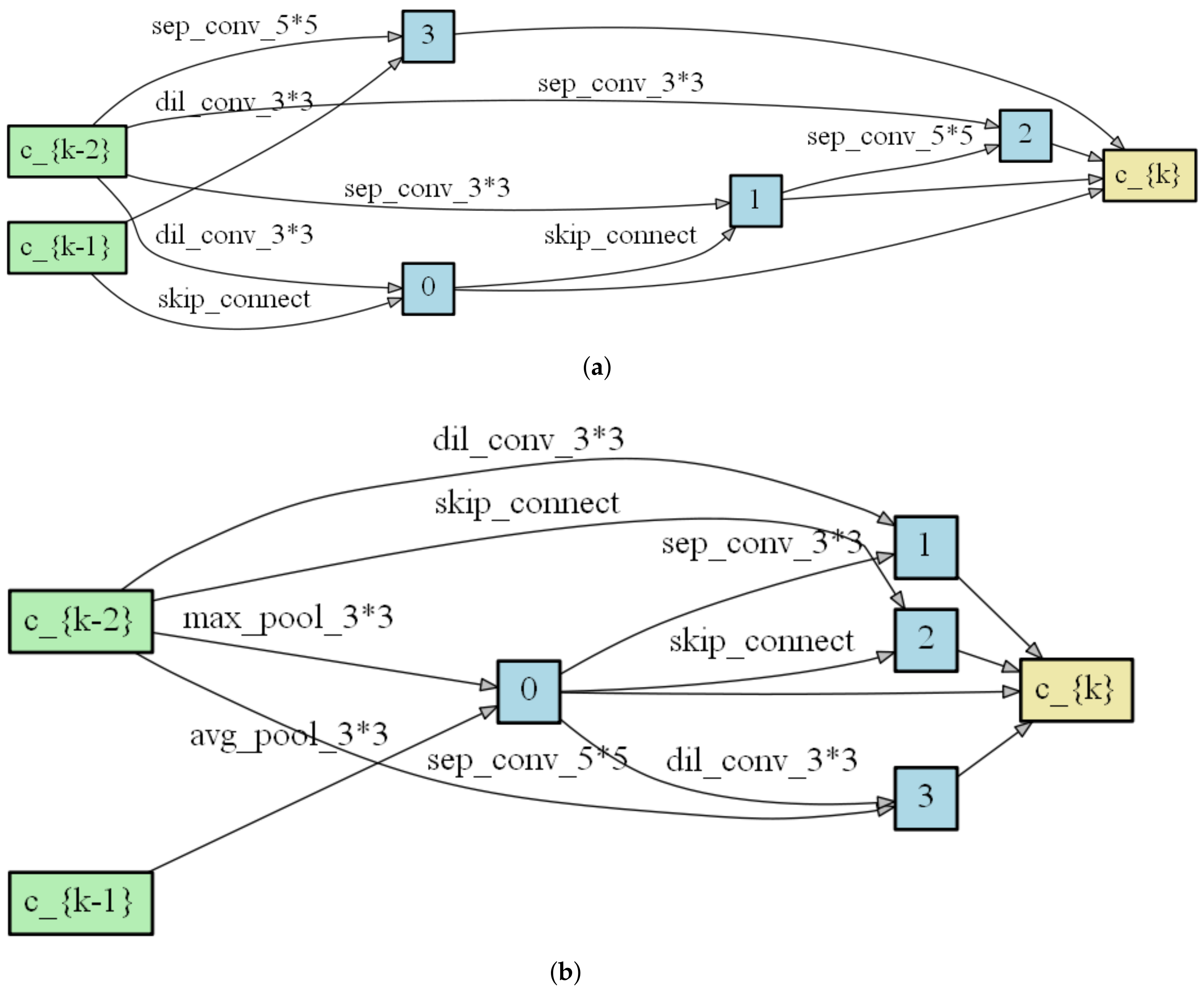
We propose a network with 10 cells—7 normal cells and 3 reduction cells—each containing N = 7 nodes. The search batch size is 64, with 200 search epochs and 36 initial channels. We run the network repeatedly several times with different random initial cell architectures. Then, 80 % of the train set is randomly chosen for training use and the remaining 20 % are for valid use. Adam optimizer [34] is used with a learning rate of 1 × 10 4 , weight decay of 3 × 10 4 , and momentum of 0.9 . Finally, the normal cells and reduction cells are obtained, as shown in Figure 5.
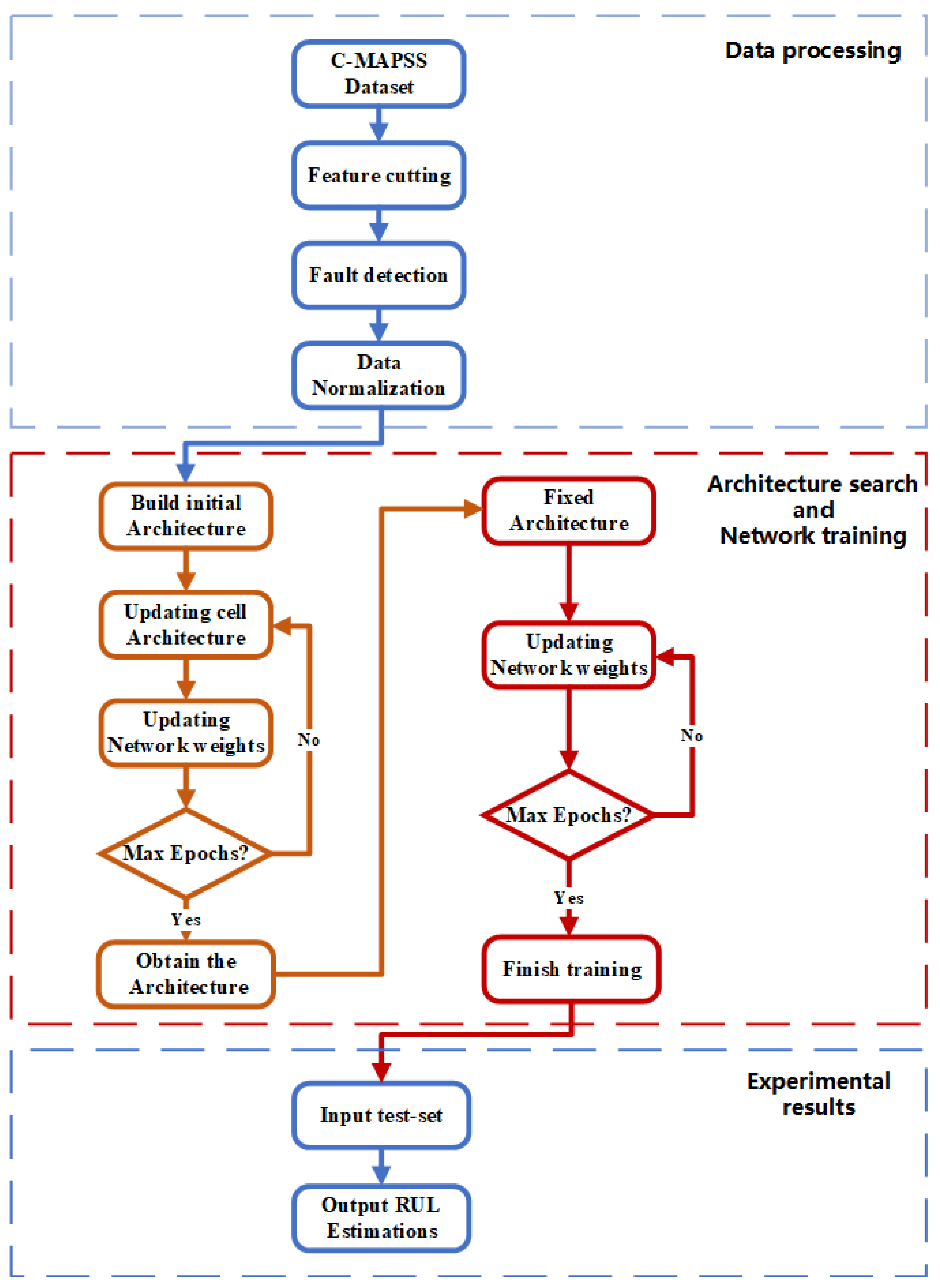
Figure 6 is a flowchart to give an introduction of our method for RUL problem. This flowchart contains three parts. The first part describes the pre-process of C-MAPSS dataset. The second part is process of network training, which includes architecture search and network weights updating. The third part is the experimental results.

4.3. Experimental Results on Single Fault Mode

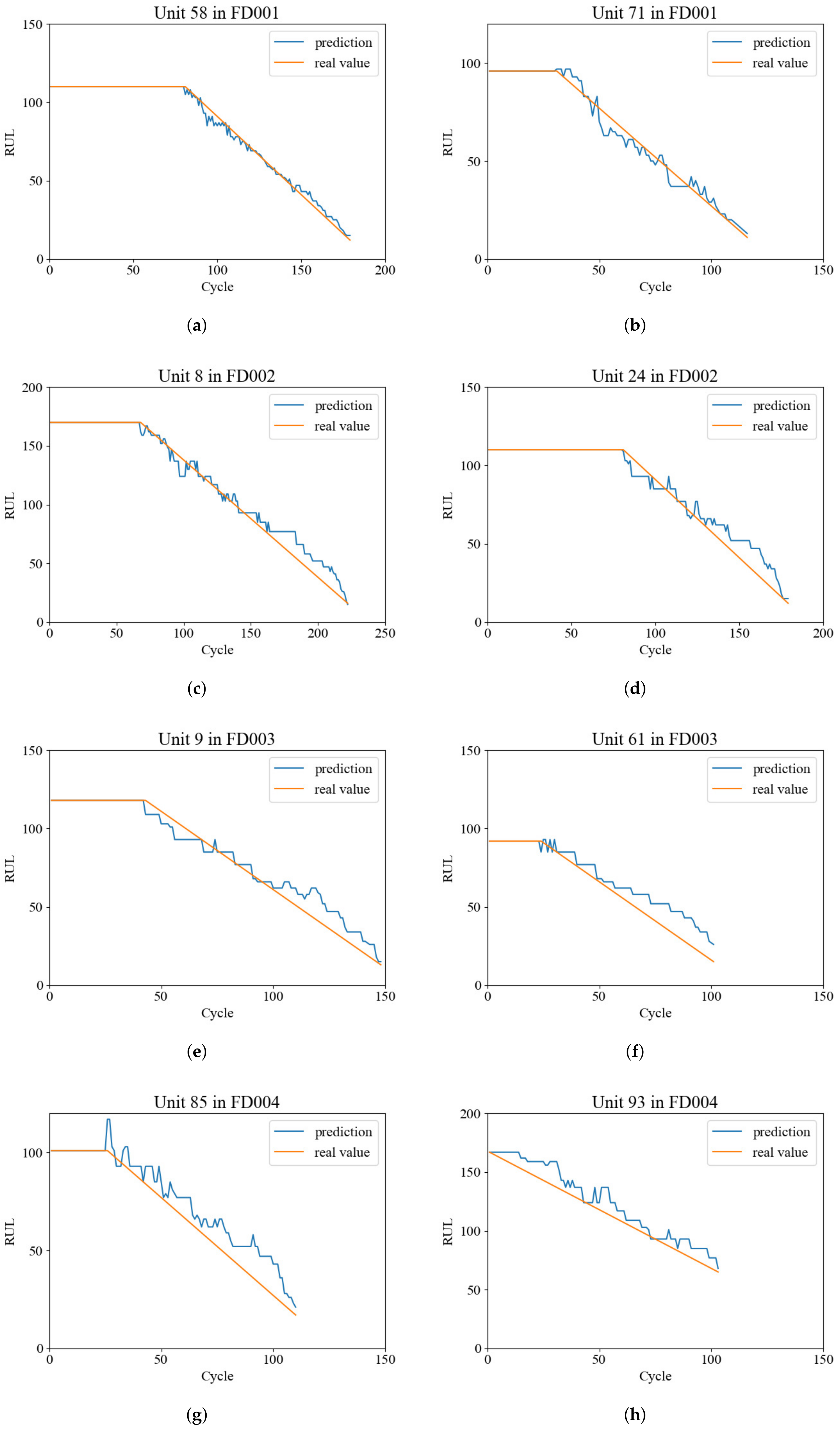
FD001 contains 100 different aero-engine units, and 4 out of the 100 units are randomly selected to show the RUL estimation results in Figure 7. The engine unit numbers are 58 and 71. As shown in the figure, the engines work normally at the initial stage. After several time steps, faults are detected with performance degradation.
In general, the estimation error is relatively higher when the system is far from complete failure. However, when the system is close to failure, the error decreases rapidly and tends close to zero. This is because in the initial stage, the data attenuation is small, and the healthy features are stronger. When the system is close to zero, the signal damping is enhanced, and the fault features are easily captured by the networks, so the error is relatively lower. Moreover, all the test data end before zero because the last part of the entire cycle is not provided.

4.4. Experimental Results on Multiple Fault Modes

As shown in Table 2, in FD001, the fault mode and working condition are simple, but the fault modes and working conditions are more complicated and hard to deal with in dataset FD002–FD004. In FD002, the working conditions vary from a sea level environment to a high-altitude, high-speed environment; in FD003, the fault modes contains both HPC degradation and fan degradation; in FD004, the problem is a collection of all the two faults modes and six working conditions. Because of the different fault modes and working conditions, the tendencies of sensors in FD002–FD004 are different and complex, and the process of feature cutting is the same as in Section 3.2, so the data processing procedure is omitted here.
We list the estimation results in Figure 7, which are randomly chosen from FD002 to FD004. Because of the single fault mode and the large scale of training set, the result on FD002 achieves excellent performance, and the error varies in a very small range during the whole life span. In FD003 and FD004, the absolute error grows larger in the beginning then descends slowly with the growth of the life cycle. Generally, due to the complexity of the fault modes and working conditions, the estimation accuracy result of the last three datasets is relatively lower than in FD001. In addition, the average life span of the last three datasets is larger than in FD001, so the absolute error is bigger. However, with the time approaching the end of a life span, the local error descends remarkably, and the local relative error is basically equal with it in FD001. For a brief summary, the proposed network is able to give an accurate estimation of the RUL problem in both the simple fault condition and complicated fault condition.
In this study, a particular performance index is proposed to evaluate the network performance: local estimation accuracy A c c . A c c is defined as the estimation error within a particular RUL cycle interval. For instance, when the system is less than 50 cycles away from complete failure, A c c i is defined as the estimation accuracy under the condition: if the absolute discrepancy between the real remaining life value R U L r e a l and the prediction value R U L e s t i is less than i cycles, which means when | R U L e s t i R U L r e a l | i , the estimation is regarded as correct.
We select A c c 5 , A c c 3 , and A c c 1 under the conditions that the system is less than 50, 20, and 10 cycles away from failure, and the prediction accuracy is illustrated in Table 3. In fact, when the system is far from complete failure, a relatively higher error is tolerable. However, when the system is close to failure, the estimation error has to be limited to a lower value, since a higher error may be a threat on the safety of both aircraft engines and aeroplanes, which may lead to unacceptable disasters. In subset FD001, when the engine unit is less than 50 cycles away from failure, 80 % of the estimation errors are limited within ± 5 cycles; when it is less than 10 cycles away, more than 88 % of the estimation errors are limited within ± 1 cycles. In subsets FD002 to FD004, the absolute errors are relatively higher than in subset FD001, and this result is in correspondence with the performance in Figure 7.

4.5. Other Effective Factors

Generally, there are four factors that have an effect on the test performance: the size of the time window, network layers, training epochs, and channels. The effects of these factors are as follows.
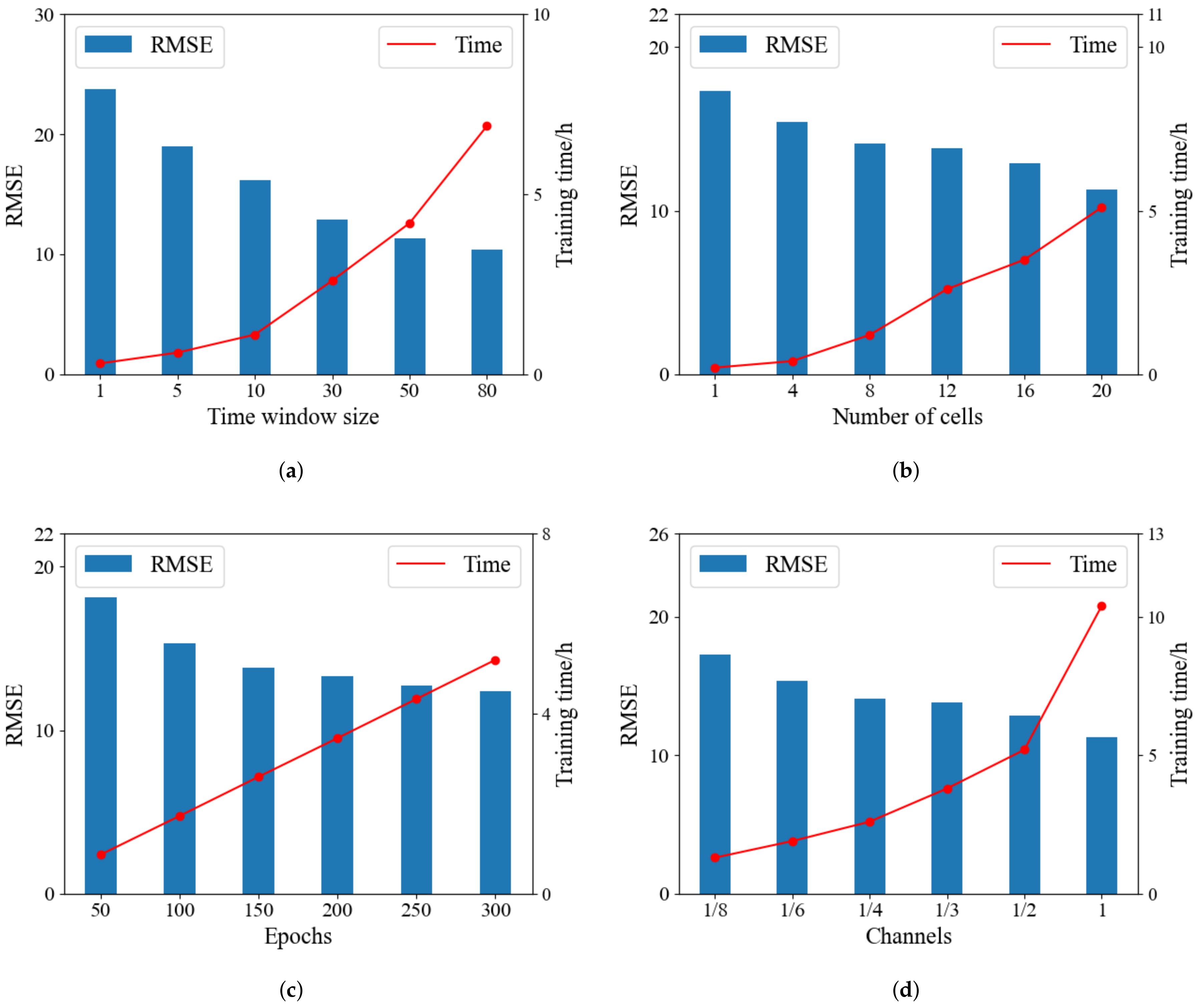
The size of the time window has an important effect on RUL performance. A large time window implies that the time data sequences can obtain more information from the previous sequence, and develops a strong connection between the present and previous sequences. However, two additional factors limit the size of the time window. As shown in Figure 8a, an increase in the time window apparently enhances the experimental time. Another factor is the dataset itself. According to Figure 2, in subset FD0001, the shortest engine unit has only 31 cycles, followed by FD002 to FD004 for which the shortest unit cycles are 21, 38, and 19, respectively. Considering these two factors, the window size is set to 30 for the four subsets. The engine unit with fewer than 30 cycles is filled with zeros at the beginning of the time steps.
The number of network layers and the training epoch play another two important roles. In our method, the depth of the network is determined by both the number of nodes in a cell and the number of cells. Table 4, Table 5, Table 6 and Table 7 show the influence of different depths on the experimental results. Because of the larger scale of samples and complex working conditions, the depths in subsets FD002 and FD004 are higher than in FD001 and FD003. An increase in the network depth can help to obtain better results on RMSE and scoring function, but with an ascent in training time. To achieve a balance between performance and training time, and also prevent overfitting, we set depth d = 70 for subset FD001 and FD003, and d = 160 for FD002 and FD004. Training epoch is set for 200. Figure 8b,c show the influence of these two factors.
The partial channels method was proposed to accelerate the searching and training process of DARTS by sampling a small part of the super network to reduce the redundancy in exploring the network space [26]. Here, we define a binary signal b i , j , which assigns 1 to selected channels and 0 to skipped ones. The selected channels are sent into computation as usual, while the skipped ones are directly copied to the output:
f i , j p c ( x i ; b i , j ) = o O e x p ( α o i , j ) o O e x p ( α o i , j ) o ( b i , j x i ) + ( 1 b i , j ) x i .
In the partial channels step, all the channels in the cells are randomly chosen for optimization. However, the uncertainty of the randomness may cause unstable searching results. To retard this problem, edge normalization is proposed:
x j p c = i < j e x p ( β o i , j ) h < j e x p ( β o h , j ) f i , j ( x i ) ,
where β is introduced to reinforce searching stability. Thus, every edge is parameterized with both α and β , making the architecture less sensitive.
In the operation selection step, we regard K as a hyperparameter, and thereafter, only 1 / K of the channels are randomly selected. By reducing the number of channels, we can select a larger batch size and reduce the experimental time. Figure 8d shows the relationship between channels, RMSE, and the training time. In our experiment, we select K = 6 .

4.6. Compared with Other Related Researches

The C-MAPSS dataset in widely used in the study of the RUL problem, with many research works published in recent years. To show the superiority of the performance, Table 8 reports the estimation results of our proposed method and other popular works. All the experimental results in this table are the best results provided from the references. Our method has a similar scale in network layers, time window size, training batch size and other hyperparameters with all the referenced studies. It is obvious to see that the estimation result of our proposed method achieves the best performance over all these popular works. Whatever the prognostic approach used, both of the score functions in subsets FD002 and FD004 are much higher than in subsets FD001 and FD003, due to the mixed conditions of the fault mode and operation conditions. DARTS achieves lower RMSE and scoring functions in all the popular works.

5. Conclusions

In this study, we introduce an autoML approach to design a network architecture based on gradient descent, to solve the RUL estimation problem on the C-MAPSS dataset. In the data processing stage, a fault detector is proposed to determine when the fault occurred. We construct the whole search space as a DAG, where each subgraph of the DAG represents a network architecture. Thereafter, we relax the search space into a continuous form by using a softmax function, then the search space and loss function become continuous and differentiable, so gradient descent can be used for optimization in the searching process. In the architecture search step, a particular group of normal convolutional cells and reduction cells are well searched for subsequent network weights training. Finally, a partial channel connection method is introduced to accelerate the searching efficiency. Compared with other related work on the C-MAPSS dataset, our proposed method achieves better performance on all four subsets, with a lower RMSE function and a lower scoring function. Moreover, the local estimation accuracy is proposed to evaluate the network performance. To take an average estimation accuracy of the four subsets, when the system is less than 50 cycles away from complete failure, the accuracy A c c 5 is up to 60.0 % under an error of ± 5 cycles, and A c c 1 is 22 % under a error of ± 1 cycle. When the system is less than 10 cycles away from failure, the accuracy A c c 5 is up to 87 % and A c c 1 is up to 68 % . As a result, with the system approaching failure, A c c becomes higher. That is to say, when the engine approaches failure, the estimation accuracy is at a very high level.

Author Contributions

Conceptualization, P.M.; methodology, P.M.; writing—original draft preparation, P.M.; writing—review and editing, P.M.; software, S.X.; investigation and supervision, B.Z.; validation and funding acquisition, Y.L. All authors have read and agreed to the published version of the manuscript.

Funding

This work was supported by the National Natural Science Foundation of China (NSFC) under Grant 62073197, Grant 61933006, and the Special Funding for Top Talents of Shandong Province.

Institutional Review Board Statement

Not applicable.

Informed Consent Statement

Not applicable.

Data Availability Statement

Not applicable.

Conflicts of Interest

The authors declare no conflict of interest.

References

  1. Si, X.; Wang, W.; Hu, C.; Zhou, D. Remaining useful life estimation—A review on the statistical data driven approaches. Eur. J. Oper. Res. 2011, 213, 1–14. [Google Scholar] [CrossRef]
  2. Saxena, A.; Simon, D. Damage Propagation Modeling for Aircraft Engine Run-to-Failure Simulation. In Proceedings of the International Conference on Prognostics and Health Management, Denver, CO, USA, 6–9 October 2008. [Google Scholar]
  3. LeCun, Y.; Bengio, Y.; Hinton, G.E. Deep learning. Nature 2015, 521, 436–444. [Google Scholar] [CrossRef] [PubMed]
  4. Heimes, F.O. Recurrent Neural Networks for Remaining Useful Life Estimation. In Proceedings of the International Conference on Prognostics and Health Management, Denver, CO, USA, 6–9 October 2008. [Google Scholar]
  5. Peel, L. Data Driven Prognostics using a Kalman Filter Ensemble of Neural Network Models. In Proceedings of the International Conference on Prognostics and Health Management, Denver, CO, USA, 6–9 October 2008. [Google Scholar]
  6. Sutskever, I.; Martens, J.; Hinton, G.E. Generating text with recurrent neural networks. In Proceedings of the 28th International Conference on Machine Learning, Bellevue, WA, USA, 28 June–2 July 2011. [Google Scholar]
  7. Sutskever, I.; Hinton, G.E.; Taylor, G.W. The recurrent temporal restricted boltzmann machine. In Proceedings of the Advances in Neural Information Processing Systems, Vancouver, BC, CA, 8–10 December 2008; pp. 1601–1608. [Google Scholar]
  8. Krizhevsky, A.; Sutskever, I.; Hinton, G.E. ImageNet Classification with Deep Convolution Neural Networks. In Proceedings of the 25th International Conference on Neural Information Processing Systems, Lake Tahoe, NV, USA, 3–6 December 2012. [Google Scholar]
  9. Khishe, M.; Caraffini, F.; Kuhn, S. Evolving Deep Learning Convolutional Neural Networks for Early COVID-19 Detection in Chest X-ray Images. Mathematics 2021, 9, 1002. [Google Scholar] [CrossRef]
  10. Jaeger, H.; Haas, H. Harnessing nonlinearity: Predicting chaotic systems and saving energy in wireless communication. Science 2004, 304, 78–80. [Google Scholar] [CrossRef] [PubMed] [Green Version]
  11. Hochreiter, S.; Schmidhuber, J. Long short-term memory. Neural Comput. 1997, 9, 1735–1780. [Google Scholar] [CrossRef]
  12. Zoph, B.; Vasudevan, V.; Shlens, J.; Le, Q.V. Learning transferable architectures for scalable image recognition. In Proceedings of the Conference on Computer Vision and Pattern Recognition, Salt Lake City, UT, USA, 18–22 June 2018. [Google Scholar]
  13. Baker, B.; Gupta, O.; Naik, N.; Raskar, R. Designing neural network achitectures using reinforcement learning. In Proceedings of the International Conference on Learning Representations, Toulon, France, 24–26 April 2017. [Google Scholar]
  14. Tan, R.Z.; Chew, X.Y.; Khaw, K.W. Neural Architecture Search for Lightweight Neural Network in Food Recognition. Mathematics 2021, 9, 1245. [Google Scholar] [CrossRef]
  15. Elsken, T.; Metzen, J.H.; Hutter, F. Neural Architecture Search: A Survey. J. Mach. Learn. Res. 2019, 20, 1997–2017. [Google Scholar]
  16. Zoph, B.; Le, Q.V. Neural architecture search with reinforcement learning. In Proceedings of the International Conference on Learning Representations, Toulon, France, 24–26 April 2017. [Google Scholar]
  17. Zhong, Z.; Yang, Z.C.; Deng, B.Y.; Yan, J.J.; Wu, W.; Shao, J.; Liu, C.L. BlockQNN: Efficient Block-Wise Neural Network Architecture Generation. IEEE Trans. Pattern Anal. Mach. Intell. 2021, 43, 7. [Google Scholar] [CrossRef] [Green Version]
  18. Geoffrey, F.M.; Peter, M.T.; Shailesh, U.H. Designing neural networks using Genetic Algorithms. In Proceedings of the 3rd International Conference on Genetic Algorithms, San Francisco, CA, USA, 1 June 1989. [Google Scholar]
  19. Peter, J.A.; Gregory, M.S.; Jordan, B.P. An evolutionary algorithm that constructs recurrent neural networks. IEEE Trans. Neural Netw. 1994, 5, 54–65. [Google Scholar]
  20. Kenneth, O.S.; Risto, M. Evolving neural networks through augmenting topologies. Evol. Comput. 2002, 10, 99–127. [Google Scholar]
  21. Liu, Y.Q.; Sun, Y.N.; Xue, B.; Zhang, M.J.; Yen, G.G.; Tan, K.C. A Survey on Evolutionary Neural Architecture Search. arXiv 2021, arXiv:2008.10937. [Google Scholar]
  22. Kevin, S.; David, D.; Jasper, S.; Hutter, F.; Osborne, M.A. Raiders of the lost architecture: Kernels for bayesian optimization in conditional parameter spaces. In Proceedings of the NIPS Workshop on Bayesian Optimization in Theory and Practice, Lake Tahoe, NV, USA, 10 December 2013. [Google Scholar]
  23. Kandasamy, K.; Neiswanger, W.; Schneider, J.; Póczos, B.; Xing, E.P. Neural architecture search with bayesian optimisation and optimal transport. arXiv 2019, arXiv:1802.07191. [Google Scholar]
  24. Liu, H.X.; Simonyan, K.; Yang, Y.M. Darts: Differentiable architecture search. In Proceedings of the International Conference on Learning Representations, New Orleans, LA, USA, 6–9 May 2019. [Google Scholar]
  25. Liang, H.W.; Zhang, S.F.; Sun, J.C.; He, X.Q.; Huang, W.R.; Zhuang, K.C.; Li, Z.G. DARTS+: Improved Differentiable Architecture Search with Early Stopping. arXiv 2019, arXiv:1909.06035v1. [Google Scholar]
  26. Xu, Y.H.; Xie, L.X.; Zhang, X.P.; Chen, X.; Qi, G.J.; Tian, Q.; Xiong, H.K. PC-DARTS: Partial Channel Connections for Memory-Efficient Architecture Search. arXiv 2020, arXiv:1907.05737v4. [Google Scholar]
  27. Deng, F.; Bi, Y.; Liu, Y.; Yang, S. Deep-Learning-Based Remaining Useful Life Prediction Based on a Multi-Scale Dilated Convolution Network. Mathematics 2021, 9, 3035. [Google Scholar] [CrossRef]
  28. Zhao, J.K.; Zhang, R.F.; Zhou, Z.; Chen, S.; Jin, J.; Liu, Q.F. A neural architecture search method based on gradient descent for remaining useful life estimation. Neurocomputing 2021, 438, 184–194. [Google Scholar] [CrossRef]
  29. Moa, H.; Custode, L.L.; Iacca, G. Evolutionary neural architecture search for remaining useful life prediction. Appl. Soft Comput. 2021, 108, 107474. [Google Scholar] [CrossRef]
  30. Cai, H.; Chen, T.Y.; Zhang, W.N.; Yu, Y.; Wang, J. Efficient architecture search by network transformation. arXiv 2017, arXiv:1070.004873. [Google Scholar]
  31. Cai, H.; Yang, J.C.; Zhang, W.N.; Han, S.; Yu, Y. Path-Level Network Transformation for Efficient Architecture Search. In Proceedings of the International Conference on Machine Learning, Stockholm, Sweden, 10–15 July 2018. [Google Scholar]
  32. Wu, Y.T.; Yuan, M.; Dong, S.P.; Lin, L.; Liu, Y.Q. Remaining useful life estimation of engineered systems using vanilla LSTM neural networks. Neurocomputing 2018, 275, 167–179. [Google Scholar] [CrossRef]
  33. Hartigan, J.A.; Wong, M.A. Algorithm AS 136: A K-Means Clustering Algorithm. J. R. Stat. Soc. 1979, 28, 100–108. [Google Scholar] [CrossRef]
  34. Kingma, D.P.; Ba, J.L. Adam: A Method for Stochastic Optimization. In Proceedings of the International Conference on Learning Representations, San Diego, CA, USA, 7–9 May 2015. [Google Scholar]
  35. Ramasso, E. Investigating computational geometry for failure prognostics. Int. J. Progn. Health Manag. 2014, 5, 005. [Google Scholar] [CrossRef]
  36. Babu, G.S.; Zhao, P.; Li, X.L. Deep convolutional neural network based regression approach for estimation of remaining useful life. In Proceedings of the International Conference on Database Systems for Advanced Applications, Dallas, TX, USA, 16–19 April 2016; pp. 214–228. [Google Scholar]
  37. Zhang, C.; Lim, P.; Qin, A.K.; Tan, K.C. Multiobjective deep belief networks ensemble for remaining useful life estimation in prognostics. IEEE Trans. Neural Netw. Learn. Syst. 2016, 99, 2306–2318. [Google Scholar] [CrossRef] [PubMed]
  38. Li, X.; Ding, Q.; Sun, J.Q. Remaining useful life estimation in prognostics using deep convolution neural networks. Reliab. Eng. Syst. Saf. 2018, 172, 1–11. [Google Scholar] [CrossRef] [Green Version]
  39. Wang, J.; Wen, G.; Yang, S.; Liu, Y. Remaining useful life estimation in prognostics using deep bidirectional LSTM neural network. In Proceedings of the Prognostics and System Health Management Conference, Chongqing, China, 26–28 October 2018; pp. 1037–1042. [Google Scholar]
  40. Singh, S.K.; Kumar, S.; Dwivedi, J.P. A novel soft computing method for engine rul prediction. Multimed. Tools Appl. 2017, 78, 4065–4087. [Google Scholar] [CrossRef]
  41. Al-Dulaimia, A.; Zabihia, S.; Asifa, A.; Mohammadib, A. A multimodal and hybrid deep neural network model for Remaining Useful Life estimation. Comput. Ind. 2019, 108, 186–196. [Google Scholar] [CrossRef]
  42. Ellefsen, A.L.; Bjørlykhauga, E.; Æsøya, V.; Ushakovb, S.; Zhanga, H.X. Remaining useful life predictions for turbofan engine degradation using semi-supervised deep architecture. Reliab. Eng. Syst. Saf. 2019, 183, 240–251. [Google Scholar] [CrossRef]
  43. Li, J.; Li, X.; He, D. A directed acyclic graph network combined with CNN and LSTM for remaining useful life prediction. IEEE Access 2019, 7, 75464–75475. [Google Scholar] [CrossRef]
  44. Deng, K.Y.; Zhang, X.Y.; Cheng, Y.J.; Zheng, Z.Y.; Jiang, F.; Liu, W.R.; Peng, J. A remaining useful life prediction method with long-short term feature processing for aircraft engines. Appl. Soft Comput. J. 2020, 93, 106344. [Google Scholar] [CrossRef]
  45. Mo, H.; Lucca, F.; Malacarne, J.; Iacca, G. Multi-Head CNN-LSTM with Prediction Error Analysis for Remaining Useful Life Prediction. In Proceedings of the 27th Conference of Open Innovations Association (FRUCT), Trento, Italy, 7–9 September 2020. [Google Scholar]
  46. Li, J.; He, D. A Bayesian Optimization AdaBN-DCNN Method With Self-Optimized Structure and Hyperparameters for Domain Adaptation Remaining Useful Life Prediction. IEEE Access 2020, 8, 41482–41501. [Google Scholar] [CrossRef]
Figure 3. All the 21 sensors outputs in training set FD001.
Mathematics 10 00352 g003
Figure 4. Fault detection using k-means. (a) K-means scatter plot; (b) Fault detection in training set; (c) K-means scatter plot; (d) Fault detection in test set.
Mathematics 10 00352 g004
Figure 5. Architectures learned on C-MAPSS. (a) normal cell; (b) reduction cell.
Mathematics 10 00352 g005
Figure 6. Flowchart of our proposed method.
Mathematics 10 00352 g006
Figure 7. Estimation results on multiple faults modes.
Mathematics 10 00352 g007
Figure 8. The effect of other factors.
Mathematics 10 00352 g008
Table 1. Details of 21 sensors.
Sensor NumberSymbolDescriptionUnit
1T2Total temperature at fan inlet°R
2T24Total temperature at LPC outlet°R
3T30Total temperature at HPC outlet°R
4T50Total temperature at LPT outlet°R
5P2Pressure at fan inletpsia
6P15Total pressure in bypass-ductpsia
7P30Total pressure at HPC outletpsia
8NfPhysical fan speedrpm
9NcPhysical core speedrpm
10eprEngine pressure ratio(P50/P2)
11Ps30Static pressure at HPC outletpsia
12phiRatio of fuel flow to Ps30pps/psi
13NRfCorrected fan speedrpm
14NRcCorrected core speedrpm
15BPRBypass Ratio
16farBBumer fuel-air ration
17htBleedBleed Enthalpy
18 N f d Demanded fan speedrpm
19 P C N f R d Demanded corrected fan speedrpm
20W31HPT coolant bleedlbm/s
21W32LPT coolant bleedlbm/s
Table 2. Details of C-MAPSS dataset.
DatasetFD001FD002FD003FD004
Engine units100260100249
Max life span(Cycles)362378525543
Min life span(Cycles)31213819
Samples in training set20,63153,57924,72061,249
Average span in training set206213247246
Samples in test set13,09633,99116,59641,214
Average span in test set131131166166
Fault modesHPC ( 1 ) HPCHPC, Fan ( 2 ) HPC, Fan
Working conditions1616
(1) HPC represents HPC degradation. (2) Fan represents fan degradation.
Table 3. Local estimation accuracy.
Remaining Cycles50 Cycles Left20 Cycles Left10 Cycles Left
Accuracy(%) Acc 5 Acc 3 Acc 1 Acc 5 Acc 3 Acc 1 Acc 5 Acc 3 Acc 1
FD00180.057.730.284.877.455.398.294.488.5
FD00262.340.220.868.650.422.183.566.457.5
FD00370.148.925.478.266.145.493.584.978.2
FD00440.826.513.255.739.620.376.765.250.4
In this table, d = R U L e s t i R U L r e a l , and Acc i represents the predicting accuracy when | d | i .
Table 4. Effect of layers in test set FD001.
Nodes (n)Cells (c)Depth ( n c )RMSEScoring Function
563020.53773
584016.64552
5105013.32388
764214.48390
785611.65264
7107010.36215
Table 5. Effect of layers in test set FD002.
Nodes (n)Cells (c)Depth ( n c )RMSEScoring Function
886426.676530
8129622.363834
81612818.862466
1088019.062680
101212016.831917
101616016.241782
Table 6. Effect of layers in test set FD003.
Nodes (n)Cells (c)Depth ( n c )RMSEScoring Function
563020.88943
584017.57668
5105015.45411
764215.67501
785612.01284
7107011.33232
Table 7. Effect of layers in test set FD004.
Nodes (n)Cells (c)Depth ( n c )RMSEScoring Function
886427.369092
8129624.787741
81612820.454230
1088022.584436
101212018.382898
101616017.032470
Table 8. RMSE and the scoring function.
MethodYearFD001FD002FD003FD004
RMSESF (1)RMSESFRMSESFRMSESF
RUL Clipper [35]201413.27- (2)22.89-16.00-24.33-
CNN [36]201618.45129030.291360019.82160029.1624,380
Random forest [37]201617.91-29.59-20.27-31.12-
vanilla LSTM [32]201819.74-27.25-24.04-34.71-
DCNN [38]201812.6127322.361041212.6428423.3112,466
BiLSTM [39]201813.6529523.18413013.7431724.865430
Stacking ensemble [40]201916.7-25.6-18.4-26.8-
Hybrid-DNN [41]201913.0524716.65159912.2228719.832253
Semi-supervised [42]201912.5623122.73336612.1025122.662840
DAG netowrk [43]201911.9622920.34273012.4655322.433370
CatBoost [44]202013.4433924.031424513.3631524.0213,931
Multi-head CNN-LSTM [45]202012.1925919.93435012.8534322.894340
AdaBN-DCNN [46]202011.9422019.29225012.3126022.143630
GD-NAS [28]202115.45-24.91-14.35-26.43-
EA-NAS [29]202111.4821417.76168312.1025118.972712
The proposed method 10.3621516.24178211.3323217.032470
(1) SF represents for the scoring function in Equation (8). (2) ‘-’ represents for the results are not given.
Publisher’s Note: MDPI stays neutral with regard to jurisdictional claims in published maps and institutional affiliations.

