Stability and Synchronization of Fractional-Order Complex-Valued Inertial Neural Networks: A Direct Approach

Abstract

This paper is dedicated to the asymptotic stability and synchronization for a type of fractional complex-valued inertial neural network by developing a direct analysis method. First, a new fractional differential inequality is presented for nonnegative functions, which provides an effective tool for the convergence analysis of fractional-order systems. Moreover, instead of the previous separation analysis for complex-valued neural networks, a class of Lyapunov functions composed of the complex-valued states and their fractional derivatives is constructed, and some compact stability criteria are derived. In synchronization analysis, unlike the existing control schemes for reduced-order subsystems, some feedback and adaptive control schemes, formed by the linear part and the fractional derivative part, are directly designed for the response fractional inertial neural networks, and some synchronization conditions are derived using the established fractional inequality. Finally, the theoretical analysis is supported via two numerical examples.

1. Introduction

In recent decades, neural networks (NNs) have been investigated broadly because of their unique structures and the high efficiency of processing information. Currently, NNs are successfully applied to optimization calculation, automatic control, signal processing, and secure communication [1]. At the same time, many important NN models have been presented by means of the first-order differential equations, including Hopfield NNs [2], competitive NNs [3], cellular NNs [4], and bidirectional associative memory (BAM) NNs [5]. However, it was revealed that NNs depicted as the first-order systems cannot effectively simulate the working mechanism of squid semicircular canal and synapse [6]. In order to depict this kind of actual problem, Babcock and Westervelt introduced the second derivatives of the neural states into Hopfield NNs in 1987, which are said to be the inertial NNs.

Up to now, the dynamics of inertial NNs have been extensively discussed. For example, the bifurcation and chaotic behavior of inertial NNs were studied in [7]. In terms of stability and control, some results have been obtained for inertial NNs by transforming the second-order models into a couple of the first-order systems [8,9,10,11,12]. However, the order reduction technique undoubtedly leads to complicated theoretical analysis, uneconomical control design, and intricate conditions. In order to overcome this challenging problem, a nonreduced-order technique was introduced in [13] to discuss the stability and synchronization of time-delay inertial NNs by constructing Lyapunov functionals directly. Currently, this direct method has been largely used to explore the dynamics and control of inertial NNs in the field of real numbers [14,15,16,17].

Regrettably, it has been revealed that it seems to be extremely difficult to solve many practical problems for real-valued NNs. For instance, the XOR problem and the symmetry detection cannot be handled by means of real-valued NNs, but they can be successfully solved by complex-valued NNs with orthogonal decision boundary. Motivated by this, complex-valued NNs and their dynamic analysis have attracted great attention. In [18], Liu et al. studied the synchronization of coupled delayed complex-valued NNs by use of the Lyapunov stability theory. The asymptotic synchronization for complex-valued BAM NNs was studied using a differential inequality in [19]. The asymptotic synchronization of delayed complex-valued stochastic switched NNs was discussed in [20] under sampling control. In all, there are two main methods to investigate complex-valued NNs. The first one is to separate the complex-valued system into two real-valued systems [18,19,21,22,23], and the other is to directly explore the dynamics of complex-valued models in light of the theory of complex-valued numbers [24,25,26]. Evidently, the nonseparation-based method is superior in terms of simplifying theoretical analysis, controller design, and conditions.

In addition to the integer-order NNs [27,28], fractional-order NNs have also attracted much attention because fractional derivatives can accurately describe the memory and heritability of neurons [29]. Recently, the stability of fractional-order NNs has been of great concern for real-valued models [30] and complex-valued models [31]. As an important and valuable collective dynamic, synchronization of fractional-order NNs was also extensively discussed based on various control schemes, including linear feedback control [32], sliding model control [33], intermittent control [34], impulsive control [35], and adaptive control [36]. Specifically, adaptive control is an effective method to automatically tune the control gains by monitoring the states of the controlled models [37]. Consequently, control cost is essentially reduced and control performance is improved [38].

In contrast to the abundant research results of low-order fractional NNs, there seems to be few reports on the dynamics and control of inertial fractional NNs [39,40,41]. In [39], Gu et al. proposed a Lyapunov functional to discuss the stability and synchronization of Riemann-Liouville fractional-order inertial NNs by designing a feedback controller and using a reduced-order method. In [40], under the framework of Riemann–Liouville fractional derivatives; the authors analyzed the stability and $\omega$-periodicity of fractional-order inertial NNs by utilizing a reduced-order technique. Compared with Riemann–Liouville derivatives, the Caputo fractional derivative has a wider application background. In [41], under the sense of Caputo derivative, the stability and synchronization of fractional-order inertial NNs with time-varying delay were studied based on the reduced-order technique.

It is noted that the reduced-order transformation was used in existing results [39,40,41] to reduce the order of the inertial term in the fractional NNs. Correspondingly, the dimension of a couple of the reduced-order systems is double that of the original inertial NNs; this greatly increases the difficulty of theoretical analysis and the complexity of the derived results. On the other hand, in the existing work on the synchronization of fractional inertial NNs [39,41], the controllers were designed for the reduced-order NNs rather than for the original inertial NNs, which imperceptibly increases the difficulty of the implementation of the controllers. Therefore, to reduce the complexity of theoretical analysis and controller design caused by the reduced-order technique, it is valuable to develop a direct method to revisit the dynamics and control of fractional inertial NNs. In addition, the models considered in [39,40,41] are real-valued; there is still a gap for fractional complex-valued inertial NNs in terms of the dynamics and control.

Based on the above motivation, the article mainly discusses the stability and synchronization of complex-valued inertial NNs in the sense of the Caputo fractional derivative by presenting a direct analytic method. The innovative approach is summarized as follows.

(1)

An important fractional inequality in sense of the Caputo derivative is developed to ensure the convergence of nonnegative functions, which provides an effective tool for the stability and adaptive control of fractional systems.

(2)

Unlike the separate control design for reduced-order subsystems of fractional inertial NNs in [39,40,41], some compact feedback and adaptive control schemes composed of the linear part and the fractional derivative part are directly designed for the response fractional inertial NNs to achieve synchronization. Obviously, the control schemes here are more concise and more easily implemented in practice since the reduced process is avoided.

(3)

Some new Lyapunov functions, consisting of the complex-valued states and their fractional derivatives, are constructed to derive the stability and synchronization criteria. Compared with the previous separation analysis for complex-valued NNs [18,19,21,22,23], the presented direct Lyapunov method in the field of complex numbers simplifies theoretical analysis and control design and induces some compact criteria.

The rest of this article is organized as follows. Some basic preliminaries are provided in Section 2. The asymptotic stability and synchronization of fractional complex-valued inertial NNs are studied in Section 3 and Section 4. In Section 5, two examples are given to illustrate the theoretical results.

Notation 1. 

Throughout the article, $\mathfrak{N}=\{1,2,\dots ,n\},$${\mathbb{R}}^n$ is a space composed of n-dimensional real-valued column vectors, and ${\mathbb{C}}^n$ is a space composed of all n-dimensional complex-valued column vectors; ${\mathbb{R}}_{+}=[0,+\infty )$. For any $z=Re\left(z\right)+Im\left(z\right)i\in \mathbb{C}$ with $i=\sqrt{-1}$, the quadratic norm of z is defined as $\parallel z\parallel =\sqrt{z\overline{z}}$; here, $\overline{z}$ is the conjugate of z. For $Z={(z_1,z_2,\dots ,z_n)}^T\in {\mathbb{C}}^n$, the quadratic norm is defined as $\parallel Z\parallel =\sqrt{Z^{H}Z}$, where $Z^H$ is the conjugate transpose of Z.

2. Preliminaries

First, related knowledge is provided.

Definition 1 

([42]). Let function $\omega \left(t\right):{\mathbb{R}}_{+}\to \mathbb{C}$ be continuous; its Reimann–Liouville integral with fractional order $\beta >0$ is defined as

$${}_0{I}_t^{\beta }\omega \left(t\right)=\frac{1}{\Gamma \left(\beta \right)}{\int }_0^t\frac{\omega \left(\tau \right)}{{(t-\tau )}^{1-\beta }}d\tau ,$$

in which $\Gamma \left(\beta \right)$ is the Gamma function.

Definition 2 

([42]). Let function $\phi :{\mathbb{R}}_{+}\to \mathbb{C}$ be differentiable; the Caputo derivative of it with fractional order $\beta \in (0,1)$ is defined as

$${}_0^C{D}_t^{\beta }\phi \left(t\right)=\frac{1}{\Gamma (1-\beta )}{\int }_0^t\frac{{\phi }^{{}^{\prime }}\left(\tau \right)}{{(t-\tau )}^{\beta }}d\tau .$$

For convenience, ${}_0^C{D}_t^{\beta }\phi \left(t\right)$ is abbreviated as $D^{\beta }\phi \left(t\right)$.

Lemma 1 

([43]). Let $u\left(t\right)$ be continuous on ${\mathbb{R}}_{+}$, then for $t\in {\mathbb{R}}_{+}$ and $0<\beta <1$,

$${}_0{I}_t^{\beta }{D}^{\beta }u\left(t\right)=u\left(t\right)-u\left(0\right).$$

Lemma 2 

([43]). For any continuous analytic function vector $x\left(t\right)\in \mathbb{C}$ and $\beta \in (0,1)$,

$$\begin{array}{c}\hfill D^{\beta }\left[x\left(t\right)\overline{x\left(t\right)}\right]⩽x\left(t\right)\overline{D^{\beta }x\left(t\right)}+\overline{x\left(t\right)}{D}^{\beta }x\left(t\right).\end{array}$$

Lemma 3 

([44]). Assume that ${\mu }_i⩾0$ for $i\in \mathfrak{N},0⩽\alpha ⩽1$, then

$${\left(\sum _{i=1}^n{\mu }_i\right)}^{\alpha }⩽\sum _{i=1}^n{\mu }_i^{\alpha }.$$

Lemma 4 

((Bernoulli inequality) [45]). Let $x⩾-1$, $0<\alpha <1$, then

$${(1+x)}^{\alpha }⩽1+\alpha x.$$

Lemma 5. 

For two continuous differentiable functions $V\left(t\right):{\mathbb{R}}_{+}\to {\mathbb{R}}_{+}$, $W\left(t\right):{\mathbb{R}}_{+}\to {\mathbb{R}}_{+}$, if $W\left(t\right)⩽V\left(t\right)$ and there exists a positive real number $A>0$, such that

$$\begin{array}{c}\hfill {}_0^C{D}_t^{\alpha }V\left(t\right)⩽-AW\left(t\right),0<\alpha <1,\end{array}$$

(1)

then

$$\underset{t\to +\infty }{lim}W\left(t\right)=0.$$

Proof. 

From inequality (1),

$$\begin{array}{c}\hfill W\left(t\right)⩽V\left(t\right)+A{}_0{I}_t^{\alpha }W\left(t\right)⩽V\left(0\right),\end{array}$$

(2)

which indicates that $W\left(t\right)$ and ${}_0{I}_t^{\alpha }W\left(t\right)$ are bounded for $t\in R_{+}$.

It will be proved subsequently that

$$\underset{t\to +\infty }{lim}W\left(t\right)=0.$$

Otherwise, by the definition of the limit, there exist a real number ${ϵ}_0>0$ and a time sequence $\left\{h_r\right\}$, satisfying $h_1<h_2<\dots <h_r<h_{r+1}<\dots$ and ${\displaystyle \underset{r\to +\infty }{lim}{h}_r=+\infty ,}$ such that $W\left(h_r\right)>{ϵ}_0.$

Note that $W\left(t\right)$ is continuous and nonnegative; there exists a number $\eta >0$ satisfying

$$\begin{array}{c}\hfill W\left(t\right)>\frac{W\left(h_r\right)}{2}>\frac{{ϵ}_0}{2},t\in O_r=[h_r-\eta ,h_r+\eta ].\end{array}$$

(3)

Without loss of generality, assume the intervals $\{O_r,r\in Z^{+}\}$ disjoint each other and $h_1-\eta >0$, which implies that $h_r-\eta <h_r+\eta <h_{r+1}-\eta$ and $h_{r+1}-h_r>2\eta$ for $r\in Z^{+}$. Therefore, for $t=h_p+\eta$ with $p\in Z^{+}$ and $p⩾2$,

$$\begin{array}{cc}\hfill {}_0{I}_t^{\alpha }W\left(t\right)& {\displaystyle =\frac{1}{\Gamma \left(\alpha \right)}{\int }_0^{h_p+\eta }{(h_p+\eta -\tau )}^{\alpha -1}W\left(\tau \right)d\tau }\hfill \\ \hfill & {\displaystyle ⩾\frac{1}{\Gamma \left(\alpha \right)}\sum _{r=1}^p{\int }_{h_r-\eta }^{h_r+\eta }{(h_p+\eta -\tau )}^{\alpha -1}W\left(\tau \right)d\tau }\hfill \\ \hfill & {\displaystyle ⩾\frac{{ϵ}_0}{2\Gamma \left(\alpha \right)}\sum _{r=1}^p{\int }_{h_r-\eta }^{h_r+\eta }{(h_p+\eta -\tau )}^{\alpha -1}d\tau }\hfill \\ \hfill & {\displaystyle =\frac{{ϵ}_0}{2\Gamma (\alpha +1)}\sum _{r=1}^p\left[{(h_p-h_r+2\eta )}^{\alpha }-{(h_p-h_r)}^{\alpha }\right]}\hfill \\ \hfill & {\displaystyle =\frac{{ϵ}_0}{2\Gamma (\alpha +1)}\sum _{r=1}^p{(h_p-h_r+2\eta )}^{\alpha }\left[1-{\left(1-\frac{2\eta }{h_p-h_r+2\eta }\right)}^{\alpha }\right].}\hfill \end{array}$$

According to the Bernoulli inequality,

$$\begin{array}{c}\hfill {}_0{I}_t^{\alpha }W\left(t\right)⩾\frac{{ϵ}_0\eta }{\Gamma \left(\alpha \right)}\sum _{r=1}^p{(h_p-h_r+2\eta )}^{\alpha -1}.\end{array}$$

(4)

Denote $\theta =sup\{h_{r+1}-h_r\}$, then $2\eta ⩽\theta$, which combines Lemma 1, one has

$$\begin{array}{cc}\hfill {(h_p-h_r+2\eta )}^{1-\alpha }& {\displaystyle ={\left[\sum _{i=r+1}^p(h_i-h_{i-1})+2\eta \right]}^{1-\alpha }}\hfill \\ \hfill & {\displaystyle ⩽\sum _{i=r+1}^p{(h_i-h_{i-1})}^{1-\alpha }+{\left(2\eta \right)}^{1-\alpha }}\hfill \\ \hfill & {\displaystyle ⩽(p-r+1){\theta }^{1-\alpha }.}\hfill \end{array}$$

(5)

From (4) and (5), for $t=h_p+\eta$ with $p\in Z^{+}$ and $p⩾2$,

$$\begin{array}{c}\hfill {}_0{I}_t^{\alpha }W\left(t\right)⩾\frac{{ϵ}_0\eta }{\Gamma \left(\alpha \right)}\sum _{r=1}^p\frac{1}{p-r+1}{\theta }^{\alpha -1}=\frac{{ϵ}_0\eta }{\Gamma \left(\alpha \right)}{\theta }^{\alpha -1}\sum _{k=1}^p\frac{1}{k}.\end{array}$$

(6)

Note that the Harmonic series is divergent, so it follows from (6) that ${}_0{I}_t^{\alpha }W\left(t\right)$ is unbounded. This is a contradiction with the result (2). Therefore, ${\displaystyle \underset{t\to +\infty }{lim}W\left(t\right)=0.}$ □

3. Asymptotic Stability

In this section, a type of FCINNs is considered, which is depicted as

$$\begin{array}{cc}\hfill {\displaystyle D^{2\beta }{x}_p\left(t\right)=}& {\displaystyle -a_p{D}^{\beta }{x}_p\left(t\right)-b_p{x}_p\left(t\right)+\sum _{j=1}^n{c}_{pj}{f}_j\left(x_j\left(t\right)\right)+I_p\left(t\right),p\in \mathfrak{N},}\hfill \end{array}$$

(7)

where $\beta \in (0,1)$, $x_p\left(t\right)\in \mathbb{C}$ is the state variable of the pth neuron at time t, $a_p>0$, $b_p>0$, $c_{pj}\in \mathbb{C}$ is the connection weight, $f_j\left(x_j\left(t\right)\right):\mathbb{C}⟶\mathbb{C}$ represents the activation function of the jth neuron at time t, $I_p\left(t\right)\in \mathbb{C}$ is the input from outside of the NN. The initial states of system (7) are given as $x_p\left(0\right)={\phi }_p\left(0\right)$, $D^{\beta }{x}_p\left(0\right)={\psi }_p\left(0\right)$ for $p\in \mathfrak{N}$.

Definition 3. 

Let $x\left(t\right)={(x_1\left(t\right),x_2\left(t\right),\dots ,x_n\left(t\right))}^T$ and $\widehat{x}\left(t\right)={({\widehat{x}}_1\left(t\right),{\widehat{x}}_2\left(t\right),\dots ,{\widehat{x}}_n\left(t\right))}^T$ be two different solutions of system $\left(7\right)$ with different initial states $x_p\left(0\right)={\phi }_p\left(0\right),D^{\beta }{x}_p\left(0\right)={\psi }_p\left(0\right),$ and ${\widehat{x}}_p\left(0\right)={\widehat{\phi }}_p\left(0\right),D^{\beta }{\widehat{x}}_p\left(0\right)={\widehat{\psi }}_p\left(0\right)$; system (7) is called to be asymptotically stable if

$${\displaystyle \underset{t\to +\infty }{lim}\Vert x\left(t\right)-\widehat{x}\left(t\right)\Vert =0.}$$

Assumption 1. 

For any $p\in \mathfrak{N}$, there exists a number $F_p>0$ such that for any $x_1,x_2\in \mathbb{C},$

$$\parallel f_p\left(x_1\right)-f_p\left(x_2\right)\parallel ⩽F_p\parallel x_1-x_2\parallel .$$

Assumption 2. 

For each $p\in \mathfrak{N}$, there exist some nonzero constants ${\breve{\delta }}_p$, ${\breve{\xi }}_p$ and a positive number ${\eta }_p>0$ such that

$$\begin{array}{c}\hfill {\breve{\Omega }}_p<0,{\breve{\Psi }}_p^2<{\breve{\Phi }}_p{\breve{\Omega }}_p,\end{array}$$

(8)

or

$$\begin{array}{c}\hfill {\breve{\Omega }}_p⩽0,{\breve{\Phi }}_p<0,{\breve{\Psi }}_p=0,\end{array}$$

(9)

where

$$\begin{array}{cc}\hfill {\breve{\Omega }}_p& {\displaystyle =2({\breve{\delta }}_p{\breve{\xi }}_p-{\breve{\delta }}_p^2{a}_p)+\sum _{j=1}^n{\breve{\delta }}_p^2\parallel c_{pj}\parallel F_j,}\hfill \\ \hfill {\breve{\Phi }}_p& {\displaystyle =-2{\breve{\delta }}_p{b}_p{\breve{\xi }}_p+\sum _{j=1}^n\left(\right|{\breve{\delta }}_p{\breve{\xi }}_p|\parallel c_{pj}\parallel F_j+{\breve{\delta }}_j^2\parallel c_{jp}\parallel F_p+|{\breve{\delta }}_j{\breve{\xi }}_j|\parallel c_{jp}\parallel F_p),}\hfill \\ \hfill {\breve{\Psi }}_p& {\displaystyle ={\eta }_p+{\breve{\xi }}_p^2-{\breve{\xi }}_p{\breve{\delta }}_p{a}_p-{\breve{\delta }}_p^2{b}_p.}\hfill \end{array}$$

Theorem 1. 

Under Assumptions 1 and 2, the FCINN (7) is asymptotically stable.

Proof. 

For $p\in \mathfrak{N},$ let $e_p\left(t\right)=x_p\left(t\right)-{\widehat{x}}_p\left(t\right)$, then

$$\begin{array}{cc}\hfill {\displaystyle D^{2\beta }{e}_p\left(t\right)=}& {\displaystyle -a_p{D}^{\beta }{e}_p\left(t\right)-b_p{e}_p\left(t\right)+\sum _{j=1}^n{c}_{pj}\left[f_j\left(x_j\left(t\right)\right)-f_j\left({\widehat{x}}_j\left(t\right)\right)\right],i\in \mathfrak{N}.}\hfill \end{array}$$

(10)

Construct a Lyapunov function

$$\begin{array}{cc}\hfill {\displaystyle V\left(t\right)=}& {\displaystyle \sum _{p=1}^n{\eta }_p{e}_p\left(t\right)\overline{e_p\left(t\right)}+\sum _{p=1}^n({\breve{\delta }}_p{D}^{\beta }{e}_p\left(t\right)+{\breve{\xi }}_p{e}_p\left(t\right))\overline{({\breve{\delta }}_p{D}^{\beta }{e}_p\left(t\right)+{\breve{\xi }}_p{e}_p\left(t\right))}.}\hfill \end{array}$$

According to Lemma 1,

$$\begin{array}{cc}\hfill D^{\beta }V(t)⩽& {\displaystyle \sum _{p=1}^n{\eta }_p(e_p(t)\overline{D^{\beta }{e}_p(t)}+\overline{e_p(t)}{D}^{\beta }{e}_p(t))}\hfill \\ \hfill & {\displaystyle +\sum _{p=1}^n[({\breve{\delta }}_p{D}^{\beta }{e}_p(t)+{\breve{\xi }}_p{e}_p(t))(\overline{{\breve{\delta }}_p{D}^{2\beta }{e}_p(t)+{\breve{\xi }}_p{D}^{\beta }{e}_p(t)})}\hfill \\ \hfill & {\displaystyle +(\overline{{\breve{\delta }}_p{D}^{\beta }{e}_p(t)+{\breve{\xi }}_p{e}_p(t)})({\breve{\delta }}_p{D}^{2\beta }{e}_p(t)+{\breve{\xi }}_p{D}^{\beta }{e}_p(t))].}\hfill \end{array}$$

(11)

Let ${\widehat{f}}_j\left(e_j\left(t\right)\right)=f_j\left(x_j\left(t\right)\right)-f_j\left({\widehat{x}}_j\left(t\right)\right)$, according to Assumption 1,

$$\begin{array}{cc}\hfill & (\overline{{\breve{\delta }}_p{D}^{\beta }{e}_p\left(t\right)+{\breve{\xi }}_p{e}_p\left(t\right)})({\breve{\delta }}_p{D}^{2\beta }{e}_p\left(t\right)+{\breve{\xi }}_p{D}^{\beta }{e}_p\left(t\right))\hfill \\ \hfill & {\displaystyle +({\breve{\delta }}_p{D}^{\beta }{e}_p\left(t\right)+{\breve{\xi }}_p{e}_p\left(t\right))(\overline{{\breve{\delta }}_p{D}^{2\beta }{e}_p\left(t\right)+{\breve{\xi }}_p{D}^{\beta }{e}_p\left(t\right)})}\hfill \\ \hfill & {\displaystyle =2{\breve{\delta }}_p({\breve{\xi }}_p-{\breve{\delta }}_p{a}_p)\overline{D^{\beta }{e}_p\left(t\right)}{D}^{\beta }{e}_p\left(t\right)-2{\breve{\xi }}_p{b}_p{\breve{\delta }}_p\overline{e_p\left(t\right)}{e}_p\left(t\right)}\hfill \\ \hfill & {\displaystyle +\left({\breve{\xi }}_p({\breve{\xi }}_p-{\breve{\delta }}_p{a}_p)-{\breve{\delta }}_p^2{b}_p\right)\left(\overline{D^{\beta }{e}_p\left(t\right)}{e}_p\left(t\right)+\overline{e_p\left(t\right)}{D}^{\beta }{e}_p\left(t\right)\right)}\hfill \\ \hfill & {\displaystyle +2Re\left\{{\breve{\delta }}_p({\breve{\delta }}_p\overline{D^{\beta }{e}_p\left(t\right)}+{\breve{\xi }}_p\overline{e_p\left(t\right)})\sum _{j=1}^n{c}_{pj}{\widehat{f}}_j\left(e_j\left(t\right)\right)\right\}.}\hfill \end{array}$$

(12)

Substituting (12) into (11),

$$\begin{array}{cc}\hfill D^{\beta }V\left(t\right)& {\displaystyle ⩽\sum _{p=1}^{n}2({\breve{\delta }}_p{\breve{\xi }}_p-{\breve{\delta }}_p^2{a}_p)\overline{D^{\beta }{e}_p\left(t\right)}{D}^{\beta }{e}_p\left(t\right)}\hfill \\ \hfill & {\displaystyle +\sum _{p=1}^n({\eta }_p+{\breve{\xi }}_p^2-{\breve{\xi }}_p{\breve{\delta }}_p{a}_p-{\breve{\delta }}_p^2{b}_p)\left[\overline{e_p\left(t\right)}{D}^{\beta }{e}_p\left(t\right)+e_p\left(t\right)\overline{D^{\beta }{e}_p\left(t\right)}\right]}\hfill \\ \hfill & {\displaystyle -\sum _{p=1}^{n}2{\breve{\delta }}_p{b}_p{\breve{\xi }}_p\overline{e_p\left(t\right)}{e}_p\left(t\right)}\hfill \\ \hfill & {\displaystyle +2{\breve{\delta }}_{p}Re\left\{\sum _{j=1}^n{c}_{pj}{\widehat{f}}_j\left(e_j\left(t\right)\right)\left({\breve{\delta }}_p\overline{D^{\beta }{e}_p\left(t\right)}+{\breve{\xi }}_p\overline{e_p\left(t\right)}\right)\right\}.}\hfill \end{array}$$

(13)

According to Assumption 1 and the properties of the norm of complex-valued numbers,

$$\begin{array}{cc}\hfill & \sum _{p=1}^{n}2{\breve{\delta }}_{p}Re\left[\sum _{j=1}^n{c}_{pj}{\widehat{f}}_j\left(e_j\left(t\right)\right)({\breve{\delta }}_p\overline{D^{\beta }{e}_p\left(t\right)}+{\breve{\xi }}_p\overline{e_p\left(t\right)})\right]\hfill \\ \hfill & {\displaystyle =\sum _{p=1}^{n}2{\breve{\delta }}_p\left\{Re\left[\sum _{j=1}^n{c}_{pj}{\widehat{f}}_j\left(e_j\left(t\right)\right){\breve{\delta }}_p\overline{D^{\beta }{e}_p\left(t\right)}+\sum _{j=1}^n{c}_{pj}{\widehat{f}}_j\left(e_j\left(t\right)\right){\breve{\xi }}_p\overline{e_p\left(t\right)}\right]\right\}}\hfill \\ \hfill & {\displaystyle ⩽\sum _{p=1}^{n}2{\breve{\delta }}_p^2\sum _{j=1}^n\parallel c_{pj}\parallel \parallel {\widehat{f}}_j\left(e_j\left(t\right)\right)\parallel \parallel \overline{D^{\beta }{e}_p\left(t\right)}\parallel +\sum _{p=1}^{n}2|{\breve{\delta }}_p{\breve{\xi }}_p|\sum _{j=1}^n\parallel c_{pj}\parallel \parallel {\widehat{f}}_j\left(e_j\left(t\right)\right)\parallel \parallel \overline{e_p\left(t\right)}\parallel }\hfill \\ \hfill & {\displaystyle ⩽\sum _{p=1}^{n}2{\breve{\delta }}_p^2\sum _{j=1}^n\parallel c_{pj}\parallel F_j\parallel e_j\left(t\right)\parallel \parallel \overline{D^{\beta }{e}_p\left(t\right)}\parallel +\sum _{p=1}^{n}2|{\breve{\delta }}_p{\breve{\xi }}_p|\sum _{j=1}^n\parallel c_{pj}\parallel F_j\parallel e_j\left(t\right)\parallel \parallel \overline{e_p\left(t\right)}\parallel }\hfill \\ \hfill & {\displaystyle ⩽\sum _{p=1}^n\sum _{j=1}^n{\breve{\delta }}_p^2\parallel c_{pj}\parallel F_j[\overline{e_j\left(t\right)}{e}_j\left(t\right)+\overline{D^{\beta }{e}_p\left(t\right)}{D}^{\beta }{e}_p\left(t\right)]}\hfill \\ \hfill & {\displaystyle +\sum _{p=1}^n|{\breve{\delta }}_p{\breve{\xi }}_p|\sum _{j=1}^n\parallel c_{pj}\parallel F_j[\overline{e_j\left(t\right)}{e}_j\left(t\right)+\overline{e_p\left(t\right)}{e}_p\left(t\right)].}\hfill \end{array}$$

(14)

Substituting (14) into (13), one has

$$\begin{array}{cc}\hfill D^{\beta }V\left(t\right)& {\displaystyle ⩽\sum _{p=1}^{n}2({\breve{\delta }}_p{\breve{\xi }}_p-{\breve{\delta }}_p^2{a}_p)\overline{D^{\beta }{e}_p\left(t\right)}{D}^{\beta }{e}_p\left(t\right)-\sum _{p=1}^{n}2{\breve{\delta }}_p{b}_p{\breve{\xi }}_p\overline{e_p\left(t\right)}{e}_p\left(t\right)}\hfill \\ \hfill & {\displaystyle +\sum _{p=1}^n({\eta }_p+{\breve{\xi }}_p^2-{\breve{\xi }}_p{\breve{\delta }}_p{a}_p-{\breve{\delta }}_p^2{b}_p)\left[\overline{e_p\left(t\right)}{D}^{\beta }{e}_p\left(t\right)+e_p\left(t\right)\overline{D^{\beta }{e}_p\left(t\right)}\right]}\hfill \\ \hfill & {\displaystyle +\sum _{p=1}^n\sum _{j=1}^n{\breve{\delta }}_p^2\parallel c_{pj}\parallel F_j\left[\overline{e_j\left(t\right)}{e}_j\left(t\right)+\overline{D^{\beta }{e}_p\left(t\right)}{D}^{\beta }{e}_p\left(t\right)\right]}\hfill \\ \hfill & {\displaystyle +\sum _{p=1}^n|{\breve{\delta }}_p{\breve{\xi }}_p|\sum _{j=1}^n\parallel c_{pj}\parallel F_j\left[\overline{e_j\left(t\right)}{e}_j\left(t\right)+\overline{e_p\left(t\right)}{e}_p\left(t\right)\right]}\hfill \\ \hfill & {\displaystyle =\sum _{p=1}^n\left[2({\breve{\delta }}_p{\breve{\xi }}_p-{\breve{\delta }}_p^2{a}_p)+\sum _{j=1}^n{\delta }_p^2\parallel c_{pj}\parallel F_j\right]\overline{D^{\beta }{e}_p\left(t\right)}{D}^{\beta }{e}_p\left(t\right)}\hfill \\ \hfill & {\displaystyle +\sum _{p=1}^n\left[-2{\breve{\delta }}_p{b}_p{\breve{\xi }}_p+\sum _{j=1}^n\left(|{\breve{\delta }}_p{\breve{\xi }}_p|\parallel c_{pj}\parallel F_j+{\breve{\delta }}_j^2\parallel c_{jp}\parallel F_p+|{\breve{\delta }}_j{\breve{\xi }}_j|\parallel c_{jp}\parallel F_p\right)\right]\overline{e_p\left(t\right)}{e}_p\left(t\right)}\hfill \\ \hfill & {\displaystyle +\sum _{p=1}^n({\eta }_p+{\breve{\xi }}_p^2-{\xi }_p{\breve{\delta }}_p{a}_p-{\breve{\delta }}_p^2{b}_p)\left[\overline{e_p\left(t\right)}{D}^{\beta }{e}_p\left(t\right)+e_p\left(t\right)\overline{D^{\beta }{e}_p\left(t\right)}\right]}\hfill \\ \hfill & {\displaystyle =\sum _{p=1}^n{\breve{\Omega }}_p\overline{D^{\beta }{e}_p\left(t\right)}{D}^{\beta }{e}_p\left(t\right)+\sum _{p=1}^n{\breve{\Phi }}_p\overline{e_p\left(t\right)}{e}_p\left(t\right)}\hfill \\ \hfill & {\displaystyle +\sum _{p=1}^n{\breve{\Psi }}_p(\overline{e_p\left(t\right)}{D}^{\beta }{e}_p\left(t\right)+e_p\left(t\right)\overline{D^{\beta }{e}_p\left(t\right)}).}\hfill \end{array}$$

(15)

For convenience, it needs to be divided into the following two cases for further discussion.

(i).

If ${\breve{\Omega }}_p<0$, according to Assumption 2,

$$\begin{array}{cc}\hfill D^{\beta }V\left(t\right)& {\displaystyle ⩽\sum _{p=1}^n{\breve{\Omega }}_p\overline{D^{\beta }{e}_p\left(t\right)}{D}^{\beta }{e}_p\left(t\right)+\sum _{p=1}^n{\breve{\Phi }}_p\overline{e_p\left(t\right)}{e}_p\left(t\right)}\hfill \\ \hfill & {\displaystyle +\sum _{p=1}^n{\breve{\Psi }}_p\left(\overline{e_p\left(t\right)}{D}^{\beta }{e}_p\left(t\right)+e_p\left(t\right)\overline{D^{\beta }{e}_p\left(t\right)}\right)}\hfill \\ \hfill & {\displaystyle =\sum _{p=1}^n[{\breve{\Omega }}_p\left(D^{\beta }{e}_p\left(t\right)+\frac{{\breve{\Psi }}_p}{{\breve{\Omega }}_p}{e}_p\left(t\right)\right)\overline{\left(D^{\beta }{e}_p\left(t\right)+\frac{{\breve{\Psi }}_p}{{\breve{\Omega }}_p}{e}_p\left(t\right)\right)}}\hfill \\ \hfill & {\displaystyle +\left({\breve{\Phi }}_p-\frac{{\breve{\Psi }}_p^2}{{\breve{\Omega }}_p}\right)\overline{e_p\left(t\right)}{e}_p\left(t\right)],}\hfill \\ \hfill & {\displaystyle ⩽\sum _{p=1}^n\left({\breve{\Phi }}_p-\frac{{\breve{\Psi }}_p^2}{{\breve{\Omega }}_p}\right)\overline{e_p\left(t\right)}{e}_p\left(t\right).}\hfill \end{array}$$

(16)

Let ${\displaystyle A_p=\frac{{\breve{\Psi }}_p^2}{{\breve{\Omega }}_p}-{\breve{\Phi }}_p>0}$ and $A=min{\left\{A_p\right\}}_{p\in \mathfrak{N}}$, we can further obtain

$$\begin{array}{c}\hfill {\displaystyle D^{\beta }V\left(t\right)⩽-\frac{A}{\overline{\eta }}\sum _{p=1}^n{\eta }_p{e}_p\left(t\right)\overline{e_p\left(t\right)},}\end{array}$$

where $\overline{\eta }=max{\left\{{\eta }_p\right\}}_{p\in \mathfrak{N}}$.

Let $W\left(t\right)={\sum }_{p=1}^n{\eta }_p\overline{e_p\left(t\right)}{e}_p\left(t\right)$, by using Lemma 5,

$$\underset{t\to +\infty }{lim}W\left(t\right)=0,$$

which implies that

$$\begin{array}{c}\hfill \underset{t\to +\infty }{lim}\Vert x\left(t\right)-\widehat{x}\left(t\right)\Vert =0.\end{array}$$

(ii).

If ${\breve{\Omega }}_p⩽0$, from condition (9),

$$\begin{array}{cc}\hfill {\displaystyle D^{\beta }V\left(t\right)}& {\displaystyle ⩽\sum _{p=1}^n{\breve{\Omega }}_p\overline{D^{\beta }{e}_p\left(t\right)}{D}^{\beta }{e}_p\left(t\right)+\sum _{p=1}^n{\breve{\Phi }}_p\overline{e_p\left(t\right)}{e}_p\left(t\right)}\hfill \\ \hfill & {\displaystyle +\sum _{p=1}^n{\breve{\Psi }}_p(\overline{e_p\left(t\right)}{D}^{\beta }{e}_p\left(t\right)+e_p\left(t\right)\overline{D^{\beta }{e}_p\left(t\right)})}\hfill \\ \hfill & {\displaystyle ⩽\sum _{p=1}^n{\breve{\Phi }}_p\overline{e_p\left(t\right)}{e}_p\left(t\right)}\hfill \\ \hfill & {\displaystyle ⩽-\frac{B}{\overline{\eta }}\sum _{p=1}^n{\eta }_p{e}_p\left(t\right)\overline{e_p\left(t\right)}}\hfill \\ \hfill & {\displaystyle =-\frac{B}{\overline{\eta }}W\left(t\right),}\hfill \end{array}$$

where $B=min{\{-{\breve{\Phi }}_p\}}_{p\in \mathfrak{N}}$. From Lemma 5,

$$\underset{t\to +\infty }{lim}W\left(t\right)=0,$$

which reveals that

$$\begin{array}{c}\hfill {\displaystyle \underset{t\to +\infty }{lim}\Vert x\left(t\right)-\widehat{x}\left(t\right)\Vert =0.}\end{array}$$

This completes the proof of Theorem 1. □

Obviously, ${\breve{\Psi }}_p=0$ if ${\eta }_p=-{\breve{\xi }}_p^2+{\breve{\xi }}_p{\breve{\delta }}_p{a}_p+{\breve{\delta }}_p^2{b}_p>0$. Assumption 2 is translated into the following form in this case.

Assumption 3. 

For any $i\in \mathfrak{N}$, there exist nonzero numbers ${\breve{\delta }}_p$, ${\breve{\xi }}_p$ satisfying

$$-{\breve{\xi }}_p^2+{\breve{\xi }}_p{\breve{\delta }}_p{a}_p+{\breve{\delta }}_p^2{b}_p>0,{\breve{\Omega }}_p⩽0,{\breve{\Phi }}_p<0.$$

Naturally, the following corollary is derived.

Corollary 1. 

Under Assumption 1 and Assumption 3, the FCINN (7) is asymptotically stable.

Obviously, ${\breve{\Psi }}_p=0$, ${\breve{\Omega }}_p={\breve{\delta }}_p^2(2-2a_p+{\sum }_{j=1}^n\parallel c_{pj}\parallel F_j)$, ${\breve{\Phi }}_p={\breve{\delta }}_p^2\{-2b_p+{\sum }_{j=1}^n(\parallel c_{pj}\parallel F_j+2\parallel c_{jp}\parallel F_p\left)\right\}$ if ${\breve{\delta }}_p={\breve{\xi }}_p$, ${\eta }_p={\breve{\delta }}_p^2(a_p+b_p-1)$, $p\in \mathfrak{N}$. Then, the following assumption is obtained from Assumption 3.

Assumption 4. 

For any $p\in \mathfrak{N}$,

$$a_p+b_p-1>0,2-2a_p+\sum _{j=1}^n\parallel c_{pj}\parallel F_j⩽0,$$

$$-2b_p+\sum _{j=1}^n(\parallel c_{pj}\parallel F_j+2\parallel c_{jp}\parallel F_p)<0.$$

Based on Assumption 4, we have the following corollary directly.

Corollary 2. 

Based on Assumptions 1 and 4, the FCINN (7) is asymptotically stable.

Remark 1. 

In [39], a Lyapunov function was selected as follows:

$$V_p\left(t\right)=\frac{1}{2}{D}^{\beta -1}\left(q_p{e}_p^2\left(t\right)\right)+\frac{1}{2}{D}^{\alpha -\beta -1}{z}_p^2+{\int }_{t-{\tau }_p}^t{m}_p{e}_p^2\left(s\right)ds.$$

Unlike the above function, a new Lyapunov function is constructed as follows:

$${\displaystyle V\left(t\right)=\sum _{p=1}^n{\eta }_p{e}_p\left(t\right)\overline{e_p\left(t\right)}+\sum _{p=1}^n({\breve{\delta }}_p{D}^{\beta }{e}_p\left(t\right)+{\breve{\xi }}_p{e}_p\left(t\right))\overline{({\breve{\delta }}_p{D}^{\beta }{e}_p\left(t\right)+{\breve{\xi }}_p{e}_p\left(t\right))},}$$

in which ${\eta }_p,$${\breve{\xi }}_p,$${\breve{\delta }}_p$ are free parameters, and the conditions of Theorem 1 are more flexible. In light of this, Assumption 3 and Assumption 4 in Corollary 1 and Corollary 2, respectively, provide two methods to verify asymptotic stability.

Remark 2. 

Currently, there have been some results to study fractional-order inertial networks [30,40,46]; a common approach in these articles is that inertial differential models are changed into first-order systems based on reduce-order transformations. Unlike that technique, a class of FCINNs is researched here and asymptotic stability is discussed directly via structuring a Lyapunov function rather than the technique of reduced order.

Remark 3. 

In [13,17,24,43,47], some results on dynamics and control for INNs described as second-order systems were presented. Compared with [13,17,24,43,47], a type of more generic models, FCINNs, is considered in this paper.

Remark 4. 

In [40], some interesting results of Mittag-Leffler stability of FCINNs were presented. In their proofs, the authors assumed that there was a nonnegative function $m\left(t\right)$ satisfying $t\ast m\left(t\right)=-d_1{D}^{-q}u\left(t\right)+d_2-u\left(t\right)$. Note that not every function can be turned into a convolution. Instead, Lemma 5 is established here to smoothly analyze the asymptotic stability of fractional-order inertial models.

Remark 5. 

Different from the separation method used in of [21,22,26,39,40,48], a Lyapunov function is designed in this article via the norm of complex-valued numbers to achieve asymptotic stability of complex-valued systems. Our work not only simplifies the theoretical analysis, but holds the feature of FCINNs without utilizing the common separation means for complex-valued models and the reduced-order idea for the fractional-order inertial system.

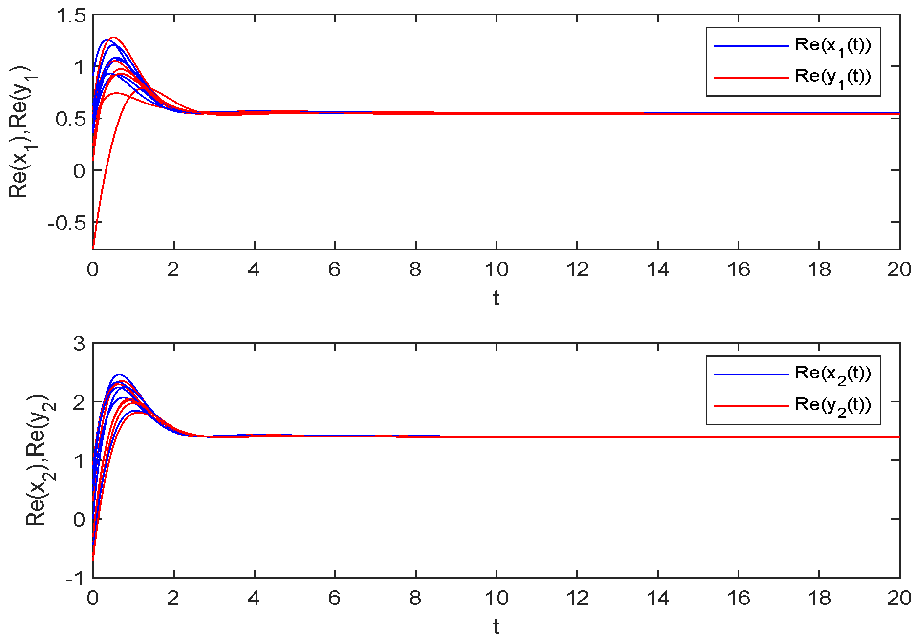
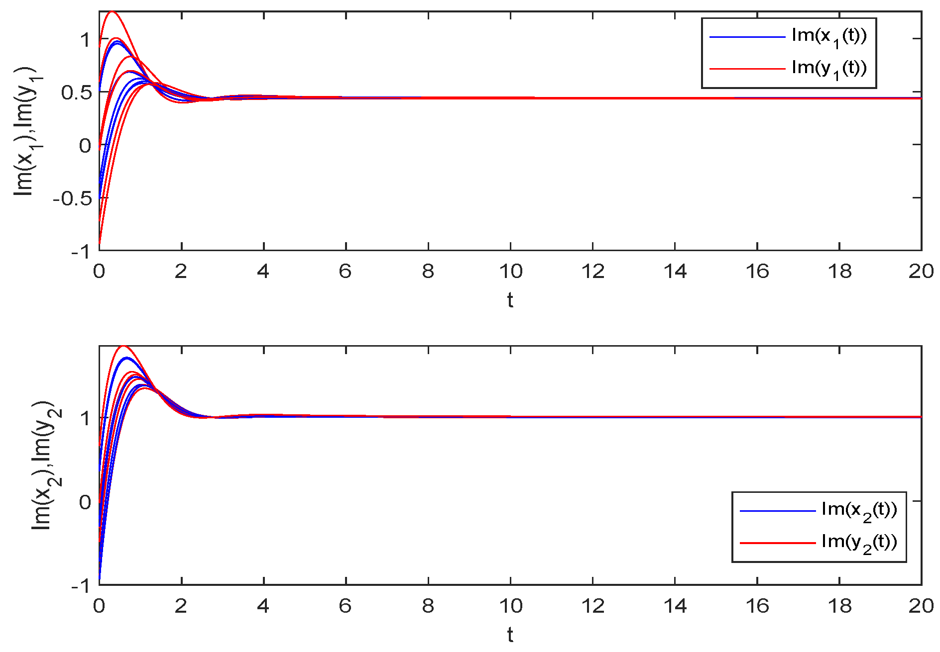
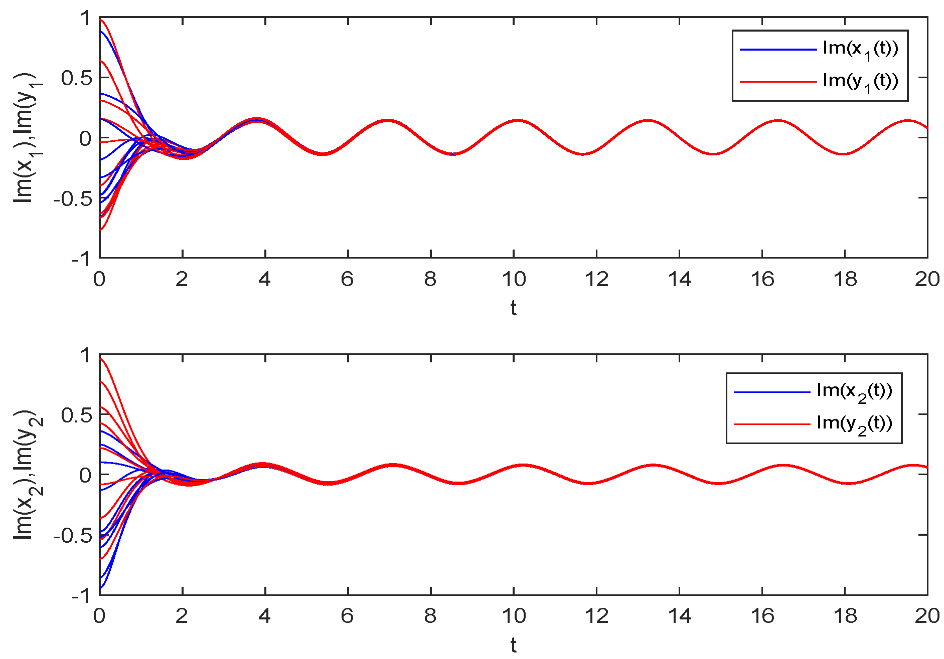
4. Asymptotic Synchronization

Let model (7) be the drive FCINN, and the response FCINN is provided as

$$\begin{array}{cc}\hfill {\displaystyle D^{2\beta }{y}_p\left(t\right)=}& {\displaystyle -a_p{D}^{\beta }{y}_p\left(t\right)-b_p{y}_p\left(t\right)+\sum _{j=1}^n{c}_{pj}{f}_j\left(y_j\left(t\right)\right)+I_p\left(t\right)+U_p\left(t\right),p\in \mathfrak{N}.}\hfill \end{array}$$

(17)

Let $z_p\left(t\right)=y_p\left(t\right)-x_p\left(t\right)$ be the synchronization error, and the error system can be easily described by

$$\begin{array}{cc}\hfill {\displaystyle D^{2\beta }{z}_p\left(t\right)=}& {\displaystyle -a_p{D}^{\beta }{z}_p\left(t\right)-b_p{z}_p\left(t\right)+\sum _{j=1}^n{c}_{pj}{\tilde{f}}_j\left(z_j\left(t\right)\right)+U_p\left(t\right),p\in \mathfrak{N},}\hfill \end{array}$$

where ${\tilde{f}}_j\left(z_j\left(t\right)\right)=f_j\left(y_j\left(t\right)\right)-f_j\left(x_j\left(t\right)\right)$.

First, the following feedback controller is developed:

$$\begin{array}{c}\hfill U_p\left(t\right)=-k_p{z}_p\left(t\right)-{\rho }_p{D}^{\beta }{z}_p\left(t\right),p\in \mathfrak{N},\end{array}$$

(18)

where $k_p>0$ and ${\rho }_p>0$ denote the control gains.

Definition 4. 

Drive-response FCINNs (7) and (17) are called to be asymptotically synchronized if

$${\displaystyle \underset{t\to +\infty }{lim}\parallel y\left(t\right)-x\left(t\right)\parallel =0,}$$

here $y\left(t\right)={(y_1\left(t\right),y_2\left(t\right),\dots ,y_n\left(t\right))}^T$ and $x\left(t\right)={(x_1\left(t\right),x_2\left(t\right),\dots ,x_n\left(t\right))}^T$.

Assumption 5. 

For any $i\in \mathfrak{N}$, there exist nonzero numbers ${\tilde{\delta }}_p$, ${\tilde{\xi }}_p$ and a positive number ${\tilde{\eta }}_p>0$ such that

$$\begin{array}{c}\hfill {\tilde{\Omega }}_p<0,{\tilde{\Psi }}_p^2<{\tilde{\Phi }}_p{\tilde{\Omega }}_p\end{array}$$

(19)

or

$$\begin{array}{c}\hfill {\tilde{\Omega }}_p⩽0,{\tilde{\Phi }}_p<0,{\tilde{\Psi }}_p=0,\end{array}$$

(20)

where

$$\begin{array}{cc}\hfill {\tilde{\Omega }}_p& {\displaystyle =2({\tilde{\delta }}_p{\tilde{\xi }}_p-{\tilde{\delta }}_p^2(a_p+{\rho }_p))+\sum _{j=1}^n{\tilde{\delta }}_p^2\parallel c_{pj}\parallel F_j,}\hfill \\ \hfill {\tilde{\Phi }}_p& {\displaystyle =-2{\tilde{\delta }}_p(b_p+k_p){\tilde{\xi }}_p+\sum _{j=1}^n\left(\right|{\tilde{\delta }}_p{\tilde{\xi }}_p|\parallel c_{pj}\parallel F_j+{\tilde{\delta }}_j^2\parallel c_{jp}\parallel F_p+|{\tilde{\delta }}_j{\tilde{\xi }}_j|\parallel c_{jp}\parallel F_p),}\hfill \\ \hfill {\tilde{\Psi }}_p& {\displaystyle ={\tilde{\eta }}_p+{\tilde{\xi }}_p^2-{\tilde{\xi }}_p{\tilde{\delta }}_p(a_p+{\rho }_p)-{\tilde{\delta }}_p^2(b_p+k_p).}\hfill \end{array}$$

Theorem 2. 

Based on Assumptions 1 and 5 and the controller (18), the FCINNs (7) and (17) realize asymptotical synchronization.

Proof. 

Construct the Lyapunov function

$$\begin{array}{cc}\hfill {\displaystyle V\left(t\right)=}& {\displaystyle \sum _{p=1}^n{\tilde{\eta }}_p{z}_p\left(t\right)\overline{z_p\left(t\right)}+\sum _{p=1}^n({\tilde{\delta }}_p{D}^{\beta }{z}_p\left(t\right)+{\tilde{\xi }}_p{z}_p\left(t\right))\overline{({\tilde{\delta }}_p{D}^{\beta }{z}_p\left(t\right)+{\tilde{\xi }}_p{z}_p\left(t\right))}.}\hfill \end{array}$$

By Lemma 1,

$$\begin{array}{cc}\hfill {\displaystyle D^{\beta }V\left(t\right)⩽}& {\displaystyle \sum _{p=1}^n{\tilde{\eta }}_p(z_p\left(t\right)\overline{D^{\beta }{z}_p\left(t\right)}+\overline{z_p\left(t\right)}{D}^{\beta }{z}_p\left(t\right))}\hfill \\ \hfill & {\displaystyle +\sum _{p=1}^n[({\tilde{\delta }}_p{D}^{\beta }{z}_p\left(t\right)+{\tilde{\xi }}_p{z}_p\left(t\right))\left(\overline{{\tilde{\delta }}_p{D}^{2\beta }{z}_p\left(t\right)+{\tilde{\xi }}_p{D}^{\beta }{z}_p\left(t\right)}\right)}\hfill \\ \hfill & {\displaystyle +\left(\overline{{\tilde{\delta }}_p{D}^{\beta }{z}_p\left(t\right)+{\tilde{\xi }}_p{z}_p\left(t\right)}\right)({\tilde{\delta }}_p{D}^{2\beta }{z}_p\left(t\right)+{\tilde{\xi }}_p{D}^{\beta }{z}_p\left(t\right))].}\hfill \end{array}$$

By Assumption 1,

$$\begin{array}{cc}\hfill D^{\beta }V\left(t\right)& {\displaystyle ⩽\sum _{p=1}^n\left[2({\tilde{\delta }}_p{\tilde{\xi }}_p-{\tilde{\delta }}_p^2(a_p+{\rho }_p))+\sum _{j=1}^n{\tilde{\delta }}_p^2\parallel c_{pj}\parallel F_j\right]\overline{D^{\beta }{z}_p\left(t\right)}{D}^{\beta }{z}_p\left(t\right)}\hfill \\ \hfill & {\displaystyle +\sum _{p=1}^n[-2{\tilde{\delta }}_p(b_p+k_p){\tilde{\xi }}_p+\sum _{j=1}^n\left(\right|{\tilde{\delta }}_p{\tilde{\xi }}_p|\parallel c_{pj}\parallel F_j+{\tilde{\delta }}_j^2\parallel c_{jp}\parallel F_p}\hfill \\ \hfill & {\displaystyle +|{\tilde{\delta }}_j{\tilde{\xi }}_j|\parallel c_{jp}\parallel F_p)]\overline{z_p\left(t\right)}{z}_p\left(t\right)}\hfill \\ \hfill & {\displaystyle +\sum _{p=1}^n\left({\tilde{\eta }}_p+{\tilde{\xi }}_p^2-{\tilde{\xi }}_p{\tilde{\delta }}_p(a_p+{\rho }_p)-{\tilde{\delta }}_p^2(b_p+k_p)\right)}\hfill \\ \hfill & {\displaystyle \times \left(\overline{z_p\left(t\right)}{D}^{\beta }{z}_p\left(t\right)+z_p\left(t\right)\overline{D^{\beta }{z}_p\left(t\right)}\right)}\hfill \\ \hfill & {\displaystyle =\sum _{p=1}^n{\tilde{\Omega }}_p\overline{D^{\beta }{z}_p\left(t\right)}{D}^{\beta }{z}_p\left(t\right)+\sum _{p=1}^n\widetilde{{\Phi }_p}\overline{z_p\left(t\right)}{z}_p\left(t\right)}\hfill \\ \hfill & {\displaystyle +\sum _{p=1}^n{\tilde{\Psi }}_p(\overline{z_p\left(t\right)}{D}^{\beta }{z}_p\left(t\right)+z_p\left(t\right)\overline{D^{\beta }{z}_p\left(t\right)}).}\hfill \end{array}$$

(21)

Similarly, the following two cases are considered.

(i).

If ${\tilde{\Omega }}_p<0$, from condition (19) and inequality (21),

$$\begin{array}{cc}\hfill {\displaystyle D^{\beta }V\left(t\right)}& {\displaystyle ⩽\sum _{p=1}^n{\tilde{\Omega }}_p\overline{D^{\beta }{z}_p\left(t\right)}{D}^{\beta }{z}_p\left(t\right)+\sum _{p=1}^n{\tilde{\Phi }}_p\overline{z_p\left(t\right)}{z}_p\left(t\right)}\hfill \\ \hfill & {\displaystyle +\sum _{p=1}^n{\tilde{\Psi }}_p\left(\overline{z_p\left(t\right)}{D}^{\beta }{z}_p\left(t\right)+z_p\left(t\right)\overline{D^{\beta }{z}_p\left(t\right)}\right)}\hfill \\ \hfill & {\displaystyle =\sum _{p=1}^n[{\tilde{\Omega }}_p\left(D^{\beta }{z}_p\left(t\right)+\frac{{\tilde{\Psi }}_p}{{\tilde{\Omega }}_p}{z}_p\left(t\right)\right)\overline{\left(D^{\beta }{z}_p\left(t\right)+\frac{{\tilde{\Psi }}_p}{{\tilde{\Omega }}_p}{z}_p\left(t\right)\right)}}\hfill \\ \hfill & {\displaystyle +\left({\tilde{\Phi }}_p-\frac{{\tilde{\Psi }}_p^2}{{\tilde{\Omega }}_p}\right)\overline{z_p\left(t\right)}{z}_p\left(t\right)],}\hfill \end{array}$$

since ${\tilde{\Psi }}_p^2<{\tilde{\Phi }}_p{\tilde{\Omega }}_p$, one has

$$\begin{array}{c}\hfill D^{\beta }V\left(t\right)⩽\sum _{p=1}^n({\tilde{\Phi }}_p-\frac{{\tilde{\Psi }}_p^2}{{\tilde{\Omega }}_p})\overline{z_p\left(t\right)}{z}_p\left(t\right).\end{array}$$

Let ${\displaystyle {\tilde{A}}_p=\frac{{\tilde{\Psi }}_p^2}{{\tilde{\Omega }}_p}-{\tilde{\Phi }}_p>0}$ and $\tilde{A}=min{\left\{{\tilde{A}}_p\right\}}_{p\in \mathfrak{N}}$, it can be obtained that

$$\begin{array}{cc}\hfill D^{\beta }V\left(t\right)& {\displaystyle ⩽-\tilde{A}\sum _{p=1}^n\overline{z_p\left(t\right)}{z}_p\left(t\right)}\hfill \\ \hfill & {\displaystyle ⩽-\frac{\tilde{A}}{\overline{\eta }}\sum _{p=1}^n{\tilde{\eta }}_p\overline{z_p\left(t\right)}{z}_p\left(t\right),}\hfill \end{array}$$

(22)

where $\overline{\eta }=max{\left\{{\tilde{\eta }}_p\right\}}_{p\in \mathfrak{N}}$.

Let $\tilde{W}\left(t\right)={\sum }_{p=1}^n{\tilde{\eta }}_p\overline{z_p\left(t\right)}{z}_p\left(t\right)$. By using Lemma 5, it is easy to get that

$$\underset{t\to +\infty }{lim}\tilde{W}\left(t\right)=0,$$

which reveals that

$$\begin{array}{c}\hfill {\displaystyle \underset{t\to +\infty }{lim}\parallel y\left(t\right)-x\left(t\right)\parallel =0.}\end{array}$$

(ii).

If ${\tilde{\Omega }}_p⩽0$, from condition (20), ${\tilde{\Phi }}_p<0$, ${\tilde{\Psi }}_p=0$,

$$\begin{array}{cc}\hfill {\displaystyle D^{\beta }V\left(t\right)}& {\displaystyle ⩽\sum _{p=1}^n{\tilde{\Omega }}_p\overline{D_t^{\beta }{z}_p\left(t\right)}{D}_t^{\beta }{z}_p\left(t\right)+\sum _{p=1}^n{\tilde{\Phi }}_p\overline{z_p\left(t\right)}{z}_p\left(t\right)}\hfill \\ \hfill & {\displaystyle +\sum _{p=1}^n{\tilde{\Psi }}_p(\overline{z_p\left(t\right)}{D}_t^{\beta }{z}_p\left(t\right)+z_p\left(t\right)\overline{D_t^{\beta }{z}_p\left(t\right)})}\hfill \\ \hfill & {\displaystyle ⩽\sum _{p=1}^n{\tilde{\Phi }}_p\overline{z_p\left(t\right)}{z}_p\left(t\right)}\hfill \\ \hfill & {\displaystyle ⩽-\tilde{B}\sum _{p=1}^n\overline{z_p\left(t\right)}{z}_p\left(t\right)}\hfill \\ \hfill & {\displaystyle ⩽-\frac{\tilde{B}}{\overline{\eta }}\sum _{p=1}^n{\tilde{\eta }}_p\overline{z_p\left(t\right)}{z}_p\left(t\right),}\hfill \end{array}$$

where $\tilde{B}=min{\{-{\tilde{\Phi }}_p\}}_{p\in \mathfrak{N}}$.

Similarly, let $\tilde{W}\left(t\right)={\sum }_{p=1}^n{\tilde{\eta }}_p\overline{z_p\left(t\right)}{z}_p\left(t\right)$; it is easy from Lemma 5 to derive that

$$\underset{t\to +\infty }{lim}\tilde{W}\left(t\right)=0,$$

which implies that

$$\begin{array}{c}\hfill {\displaystyle \underset{t\to +\infty }{lim}\parallel y\left(t\right)-x\left(t\right)\parallel =0.}\end{array}$$

This completes the proof of Theorem 2. □

Evidently, ${\tilde{\Psi }}_p=0$ if ${\tilde{\eta }}_p=-{\tilde{\xi }}_p^2+{\tilde{\xi }}_p{\tilde{\delta }}_p(a_p+{\rho }_p)+{\tilde{\delta }}_p^2(b_p+k_p)>0$, and the following assumption is given.

Assumption 6. 

For any $p\in \mathfrak{N}$, there exist nonzero numbers ${\breve{\delta }}_p$, ${\breve{\xi }}_p$ satisfying

$$-{\tilde{\xi }}_p^2+{\tilde{\xi }}_p{\tilde{\delta }}_p(a_p+{\rho }_p)+{\tilde{\delta }}_p^2(b_p+k_p)>0,{\tilde{\Omega }}_p⩽0,{\tilde{\Phi }}_p<0.$$

Based on Assumption 5, the following corollary is derived.

Corollary 3. 

Under Assumption 1, Assumption 6, and the controller (18), the FCINNs (7) and (17) achieve asymptotical synchronization.

Furthermore, ${\tilde{\Psi }}_p=0$, ${\tilde{\Omega }}_p={\tilde{\delta }}_p^2(2-2a_p-2{\rho }_p+{\sum }_{j=1}^n\parallel c_{pj}\parallel F_j)$, ${\tilde{\Phi }}_p={\tilde{\delta }}_p^2\{-2b_p-2k_p+{\sum }_{j=1}^n\left(\parallel c_{pj}\parallel F_j+2\parallel c_{jp}\parallel F_p\right)\}$ if ${\tilde{\delta }}_p={\tilde{\xi }}_p$, ${\tilde{\eta }}_p={\tilde{\delta }}_p^2(a_p+{\rho }_p+b_p+k_p-1)$, $p\in \mathfrak{N}$. Under such circumstances, Assumption 6 is simplified to the following form.

Assumption 7. 

For any $p\in \mathfrak{N}$,

$$a_p+{\rho }_p+b_p+k_p-1>0,2-2a_p-2{\rho }_p+\sum _{j=1}^n\parallel c_{pj}\parallel F_j⩽0,$$

$$-2b_p-2k_p+\sum _{j=1}^n(\parallel c_{pj}\parallel F_j+2\parallel c_{jp}\parallel F_p)<0.$$

Based on Assumption 7, the following corollary can be derived directly.

Corollary 4. 

Under Assumptions 1 and 7 and the feedback controller (18), the FCINNs (7) and (17) achieve asymptotical synchronization.

Remark 6. 

The Mittag-Leffler and asymptotic ω-periodicity of fractional-order inertial NNs was investigated by using reduced-order tool in [40]. Unlike this work, without the reduced-order means, by introducing a Lyapunov function, the asymptotic stability and synchronization are studied in this paper for FCINNs.

Remark 7. 

In [41], the synchronization control of fractional-order inertial systems was investigated, in which the following the controller was developed:

$$U_p\left(t\right)=-{\lambda }_p{e}_p\left(t\right)-{\gamma }_p{z}_p\left(t\right)-D^{\alpha -\beta }{e}_p\left(t\right).$$

Evidently, the control scheme (18) designed here is more concise.

To automatically turn the control gains, the following adaptive control scheme is designed:

$$\left\{\begin{array}{cc}{U}_p\left(t\right)\hfill & =-k_p\left(t\right)z_p\left(t\right)-{\rho }_p\left(t\right)D^{\beta }{z}_p\left(t\right),\hfill \\ D^{\beta }{k}_p\left(t\right)\hfill & ={\lambda }_p\left(z_p\left(t\right)\overline{z_p\left(t\right)}+Re[\overline{z_p\left(t\right)}{D}^{\beta }{z}_p\left(t\right)]\right),\hfill \\ D^{\beta }{\rho }_p\left(t\right)\hfill & ={\xi }_p\left(\overline{D^{\beta }{z}_p\left(t\right)}{D}^{\beta }{z}_p\left(t\right)+Re[\overline{z_p\left(t\right)}{D}^{\beta }{z}_p\left(t\right)]\right),\hfill \end{array}\right.$$

(23)

where ${\lambda }_p>0,$${\xi }_p>0$ for $p\in \mathfrak{N}$.

Theorem 3. 

Based on Assumption 1 and the adaptive feedback controller (23), the FCINNs (7) and (17) achieve asymptotical synchronization.

Proof. 

Establish a Lyapunov function

$$\begin{array}{cc}\hfill V\left(t\right)=& {\displaystyle \frac{1}{2}\sum _{p=1}^n{\widehat{\eta }}_p{z}_p\left(t\right)\overline{z_p\left(t\right)}}\hfill \\ \hfill & {\displaystyle +\frac{1}{2}\sum _{p=1}^n{\widehat{\delta }}_p(D^{\beta }{z}_p\left(t\right)+z_p\left(t\right))\overline{(D^{\beta }{z}_p\left(t\right)+z_p\left(t\right))}}\hfill \\ \hfill & {\displaystyle +\frac{1}{2}\sum _{p=1}^n\frac{{\widehat{\delta }}_p}{{\lambda }_p}{({\widehat{k}}_p-k_p\left(t\right))}^2+\frac{1}{2}\sum _{p=1}^n\frac{{\widehat{\delta }}_p}{{\xi }_p}{({\widehat{\rho }}_p-{\rho }_p\left(t\right))}^2.}\hfill \end{array}$$

(24)

From Lemma 1, we obtain

$$\begin{array}{cc}\hfill {\displaystyle D^{\beta }V\left(t\right)⩽}& {\displaystyle \frac{1}{2}\sum _{p=1}^n{\widehat{\eta }}_p(z_p\left(t\right)\overline{D^{\beta }{z}_p\left(t\right)}+\overline{z_p\left(t\right)}{D}^{\beta }{z}_p\left(t\right))}\hfill \\ \hfill & {\displaystyle +\frac{1}{2}\sum _{p=1}^n{\widehat{\delta }}_p[(D^{\beta }{z}_p\left(t\right)+z_p\left(t\right))\left(\overline{D^{2\beta }{z}_p\left(t\right)+D^{\beta }{z}_p\left(t\right)}\right)}\hfill \\ \hfill & {\displaystyle +\left(\overline{D^{\beta }{z}_p\left(t\right)+z_p\left(t\right)}\right)(D^{2\beta }{z}_p\left(t\right)+D^{\beta }{z}_p\left(t\right))]}\hfill \\ \hfill & {\displaystyle -\sum _{p=1}^n\frac{{\widehat{\delta }}_p}{{\lambda }_p}({\widehat{k}}_p-k_p\left(t\right))D^{\beta }{k}_p\left(t\right)-\sum _{p=1}^n\frac{{\widehat{\delta }}_p}{{\xi }_p}({\widehat{\rho }}_p-{\rho }_p\left(t\right))D^{\beta }{\rho }_p\left(t\right).}\hfill \end{array}$$

From Assumption 1, we obtain

$$\begin{array}{cc}\hfill D^{\beta }V\left(t\right)⩽& {\displaystyle \frac{1}{2}\sum _{p=1}^n{\widehat{\eta }}_p(z_p\left(t\right)\overline{D^{\beta }{z}_p\left(t\right)}+\overline{z_p\left(t\right)}{D}^{\beta }{z}_p\left(t\right))}\hfill \\ \hfill & {\displaystyle +\frac{1}{2}\sum _{p=1}^n{\widehat{\delta }}_p\{2(1-a_p-{\rho }_p\left(t\right))\overline{D^{\beta }{z}_p\left(t\right)}{D}^{\beta }{z}_p\left(t\right)}\hfill \\ \hfill & {\displaystyle +(1-a_p-{\rho }_p\left(t\right)-b_p-k_p\left(t\right))\left(\overline{z_p\left(t\right)}{D}^{\beta }{z}_p\left(t\right)+z_p(t\overline{)D^{\beta }}{z}_p\left(t\right)\right)}\hfill \\ \hfill & {\displaystyle -2(b_p+k_p\left(t\right))\overline{z_p\left(t\right)}{z}_p\left(t\right)}\hfill \\ \hfill & {\displaystyle +2Re[(\overline{D^{\beta }{z}_p\left(t\right)}+\overline{z_p\left(t\right)})\sum _{j=1}^n{c}_{pj}{\tilde{f}}_j\left(z_j\left(t\right)\right)]\}}\hfill \\ \hfill & {\displaystyle +\sum _{p=1}^n{\widehat{\delta }}_p(k_p\left(t\right)-{\widehat{k}}_p)\{z_p\left(t\right)\overline{z_p\left(t\right)}+Re\left[\overline{z_p\left(t\right)}{D}^{\beta }{z}_p\left(t\right)\right]\}}\hfill \\ \hfill & {\displaystyle +\sum _{p=1}^n{\widehat{\delta }}_p({\rho }_p\left(t\right)-{\widehat{\rho }}_p)\{\overline{D^{\beta }{z}_p\left(t\right)}{D}^{\beta }{z}_p\left(t\right)+Re\left[\overline{z_p\left(t\right)}{D}^{\beta }{z}_p\left(t\right)\right]\}}\hfill \\ \hfill ⩽& {\displaystyle \sum _{p=1}^n[{\widehat{\eta }}_p+{\widehat{\delta }}_p(1-a_p-{\widehat{\rho }}_p-b_p-{\widehat{k}}_p)]Re\left(\overline{z_p\left(t\right)}{D}^{\beta }{z}_p\left(t\right)\right)}\hfill \\ \hfill & {\displaystyle +\sum _{p=1}^n[-(b_p+{\widehat{k}}_p){\widehat{\delta }}_p{z}_p\left(t\right)\overline{z_p\left(t\right)}+(1-a_p-{\widehat{\rho }}_p){\widehat{\delta }}_p\overline{D^{\beta }{z}_p\left(t\right)}{D}^{\beta }{z}_p\left(t\right)]}\hfill \\ \hfill & {\displaystyle +\sum _{p=1}^n{\widehat{\delta }}_{p}Re\left[(\overline{D^{\beta }{z}_p\left(t\right)}+\overline{z_p\left(t\right)})\sum _{j=1}^n{c}_{pj}{\tilde{f}}_j\left(z_j\left(t\right)\right)\right]}\hfill \\ \hfill ⩽& {\displaystyle \sum _{p=1}^n[{\widehat{\eta }}_p+{\widehat{\delta }}_p(1-a_p-{\widehat{\rho }}_p-b_p-{\widehat{k}}_p)]Re\left(\overline{z_p\left(t\right)}{D}^{\beta }{z}_p\left(t\right)\right)}\hfill \\ \hfill & {\displaystyle +\sum _{p=1}^n[-(b_p+{\widehat{k}}_p){\widehat{\delta }}_p{z}_p\left(t\right)\overline{z_p\left(t\right)}+(1-a_p-{\widehat{\rho }}_p){\widehat{\delta }}_p\overline{D^{\beta }{z}_p\left(t\right)}{D}^{\beta }{z}_p\left(t\right)]}\hfill \\ \hfill & {\displaystyle +\sum _{p=1}^n{\widehat{\delta }}_p\sum _{j=1}^n\parallel c_{pj}\parallel F_j\parallel z_j\left(t\right)\parallel \parallel D^{\beta }{z}_p\left(t\right)\parallel }\hfill \\ \hfill & {\displaystyle +\sum _{p=1}^n{\widehat{\delta }}_p\sum _{j=1}^n\parallel c_{pj}\parallel F_j\parallel z_j\left(t\right)\parallel \parallel z_j\left(t\right)\parallel }\hfill \\ \hfill ⩽& {\displaystyle \sum _{p=1}^n[{\widehat{\eta }}_p+{\widehat{\delta }}_p(1-a_p-{\widehat{\rho }}_p-b_p-{\widehat{k}}_p)]Re\left(\overline{z_p\left(t\right)}{D}^{\beta }{z}_p\left(t\right)\right)}\hfill \\ \hfill & {\displaystyle +\sum _{p=1}^n[-(b_p+{\widehat{k}}_p){\widehat{\delta }}_p{z}_p\left(t\right)\overline{z_p\left(t\right)}+(1-a_p-{\widehat{\rho }}_p){\widehat{\delta }}_p\overline{D^{\beta }{z}_p\left(t\right)}{D}^{\beta }{z}_p\left(t\right)]}\hfill \\ \hfill & {\displaystyle +\frac{1}{2}\sum _{p=1}^n{\widehat{\delta }}_p\sum _{j=1}^n\parallel c_{pj}\parallel F_j(\overline{z_j\left(t\right)}{z}_j\left(t\right)+\overline{D^{\beta }{z}_p\left(t\right)}{D}^{\beta }{z}_p\left(t\right))}\hfill \\ \hfill & {\displaystyle +\frac{1}{2}\sum _{p=1}^n{\widehat{\delta }}_p\sum _{j=1}^n\parallel c_{pj}\parallel F_j(\overline{z_j\left(t\right)}{z}_j\left(t\right)+z_p\left(t\right)z_p\left(t\right))}\hfill \\ \hfill =& {\displaystyle \sum _{p=1}^n[{\widehat{\eta }}_p+{\widehat{\delta }}_p(1-a_p-{\widehat{\rho }}_p-b_p-{\widehat{k}}_p)]Re\left(\overline{z_p\left(t\right)}{D}^{\beta }{z}_p\left(t\right)\right)}\hfill \\ \hfill & {\displaystyle +\sum _{p=1}^n[-(b_p+{\widehat{k}}_p){\widehat{\delta }}_p+\frac{1}{2}\sum _{j=1}^n{\widehat{\delta }}_j\parallel c_{jp}\parallel F_p+\frac{1}{2}{\widehat{\delta }}_j\parallel c_{jp}\parallel F_p+\frac{1}{2}{\widehat{\delta }}_p\parallel c_{pj}\parallel F_j]z_p\left(t\right)\overline{z_p\left(t\right)}}\hfill \\ \hfill & {\displaystyle +\sum _{p=1}^n[(1-a_p-{\widehat{\rho }}_p){\widehat{\delta }}_p+\frac{1}{2}{\widehat{\delta }}_p\sum _{j=1}^n\parallel c_{pj}\parallel F_j]\overline{D^{\beta }{z}_p\left(t\right)}{D}^{\beta }{z}_p\left(t\right).}\hfill \end{array}$$

(25)

For $i\in \mathfrak{N}$, choose

$$\begin{array}{cc}\hfill {\widehat{\eta }}_p=& {\displaystyle {\widehat{\delta }}_p(a_p+{\widehat{\rho }}_p+b_p+{\widehat{k}}_p-1),}\hfill \\ \hfill {\widehat{\rho }}_p=& {\displaystyle 1-a_p+\frac{1}{2}{\widehat{\delta }}_p\sum _{j=1}^n\parallel c_{pj}\parallel F_j,}\hfill \\ \hfill \widehat{k_p}=& {\displaystyle -b_p+\frac{1}{2}\sum _{j=1}^n\frac{{\widehat{\delta }}_j}{{\widehat{\delta }}_p}\parallel c_{jp}\parallel F_p+\frac{1}{2}\parallel c_{pj}\parallel F_j+\frac{\sigma }{{\widehat{\delta }}_p},}\hfill \end{array}$$

in which $\sigma >0$. Obviously, ${\widehat{\eta }}_p>0$, and by (25),

$$\begin{array}{cc}\hfill D^{\beta }V\left(t\right)⩽& {\displaystyle -\sigma \sum _{p=1}^n\overline{z_p\left(t\right)}{z}_p\left(t\right)⩽-\frac{2\sigma }{\overline{\widehat{\eta }}}\frac{1}{2}\sum _{p=1}^n{\widehat{\eta }}_p{z}_p\left(t\right)\overline{z_p\left(t\right)},}\hfill \end{array}$$

here $\overline{\widehat{\eta }}=max{\left\{\widehat{\eta }\right\}}_{p\in \mathfrak{N}}$.

Let ${\displaystyle W\left(t\right)=\frac{1}{2}\sum _{p=1}^n{\widehat{\eta }}_p{z}_p\left(t\right)\overline{z_p\left(t\right)}}$. Obviously $W\left(t\right)⩽V\left(t\right)$, and by Lemma 5,

$$\underset{t\to +\infty }{lim}W\left(t\right)=0,$$

which reveals that

$$\begin{array}{c}\hfill {\displaystyle \underset{t\to +\infty }{lim}\parallel y\left(t\right)-x\left(t\right)\parallel =0.}\end{array}$$

 □

Remark 8. 

Note that the stability and synchronization for time-delayed inertial NNs were discussed in the sense of Riemann–Liouville in [39] using a reduced-order method. In contrast, the model considered in this article is described based on the Caputo derivative and a direct method is developed in theoretical analysis, and a new adaptive control scheme is proposed to adjust the control gains.

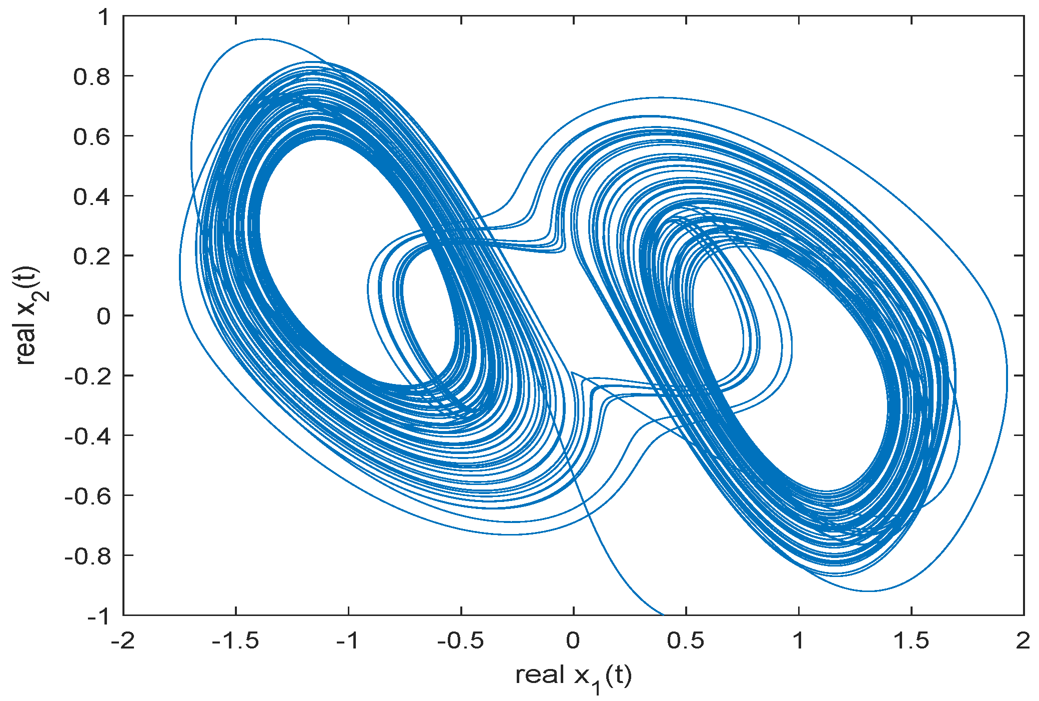
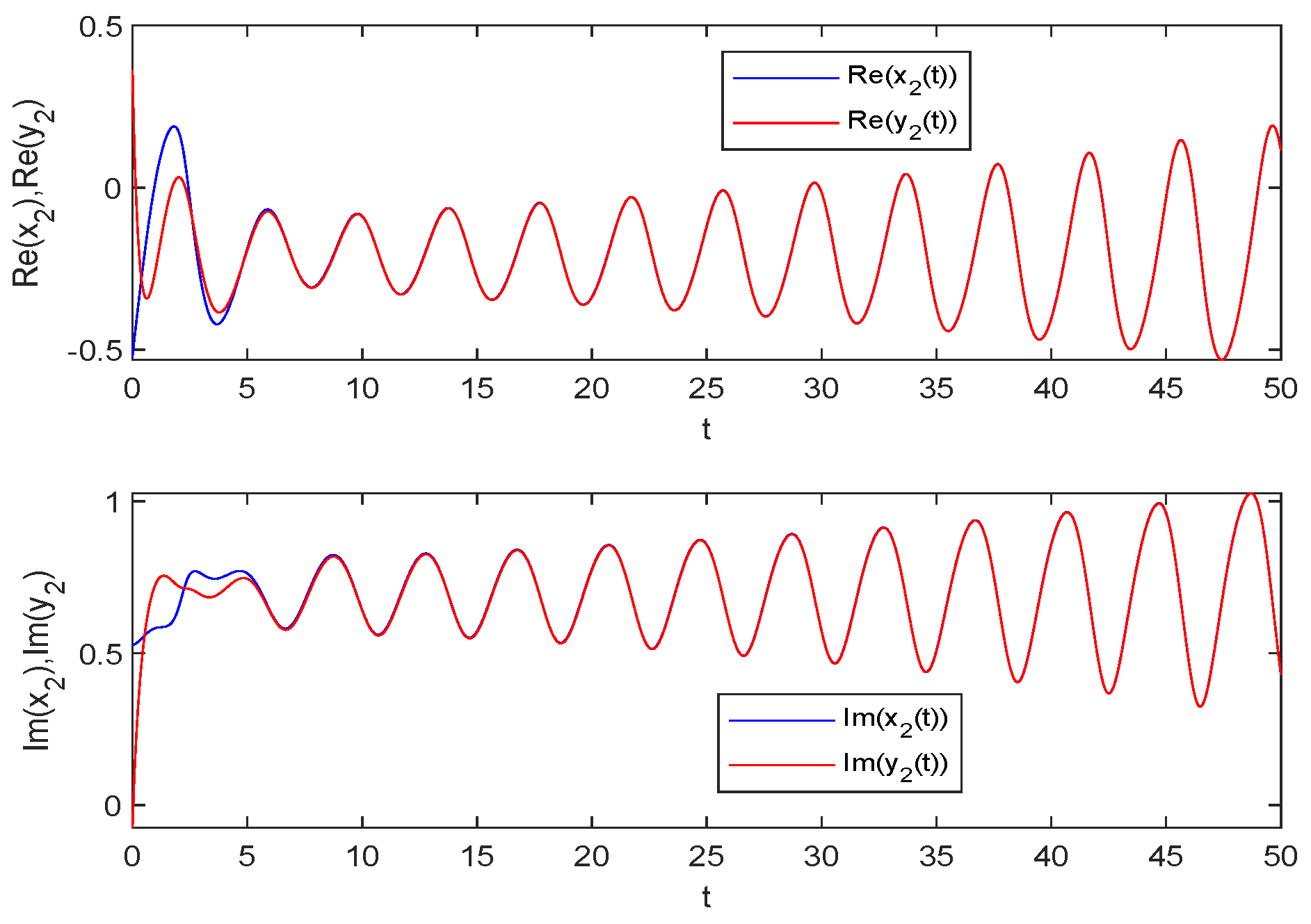
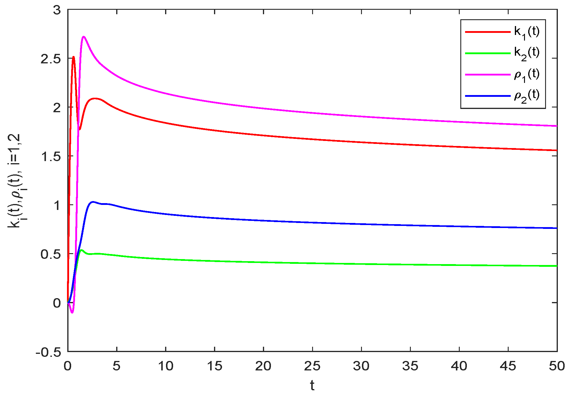
5. Numerical Simulations

Several numerical results are given here to illustrate the theoretical analysis.

Example 1. 

Considered the following FCINN:

$$\begin{array}{cc}\hfill {\displaystyle D^{2\beta }{x}_p\left(t\right)=}& {\displaystyle -a_p{D}^{\beta }{x}_p\left(t\right)-b_p{x}_p\left(t\right)+\sum _{j=1}^2{c}_{pj}{f}_j\left(x_j\left(t\right)\right)+I_p\left(t\right),p=1,2,}\hfill \end{array}$$

(26)

here $\beta =0.9$, $a_1=a_2=2$, $b_1=b_2=4$, $f_1\left(\sigma \right)=f_2\left(\sigma \right)=tanh\left(\sigma \right),$

$$C={\left(c_{pj}\right)}_{2\times 2}=\left[\begin{array}{cc}0.4-0.8i& -0.3+0.1i\\ -0.1-0.4i& 0.5+0.2i\end{array}\right].$$

By computation, $a_p+b_p-1=5>0$, $p=1,2$,

$$2-2a_1+\sum _{j=1}^2\parallel c_{1j}\parallel F_j=-0.78935⩽0,2-2a_2+\sum _{j=1}^2\parallel c_{2j}\parallel F_j=-1.0492⩽0,$$

$$-2b_1+\sum _{j=1}^2(\parallel c_{1j}\parallel F_j+2\parallel c_{j1}\parallel F_1)=-4.0798<0,$$

$$-2b_2+\sum _{j=1}^2(\parallel c_{2j}\parallel F_j+2\parallel c_{j2}\parallel F_2)=-5.3397<0,$$

the conditions of Corollary 2 are apparently satisfied, so the FCINN (26) realizes asymptotical stability, which is further demonstrated in Figure 1, Figure 2, Figure 3 and Figure 4. Here, the initial values of the NN (26) are randomly selected in $[-1,1]+[-1,1]i$, $I_1=2+2i$ and $I_2=5+4i$ in Figure 1 and Figure 2, $I_1\left(t\right)=5sin\left(2t\right)+i5sin\left(2t\right)$ and $I_2\left(t\right)=5cos\left(2t\right)+5icos\left(2t\right)$ in Figure 3 and Figure 4.

Example 2. 

Consider the following driving the FCINN:

$$\begin{array}{cc}\hfill {\displaystyle D^{2\beta }{x}_p\left(t\right)=}& {\displaystyle -a_p{D}^{\beta }{x}_p\left(t\right)-b_p{x}_i\left(t\right)+\sum _{j=1}^2{c}_{pj}{f}_j\left(x_j\left(t\right)\right),p=1,2,}\hfill \end{array}$$

(27)

and the response FCINN is depicted as

$$\begin{array}{cc}\hfill {\displaystyle D^{2\beta }{y}_p\left(t\right)=}& {\displaystyle -a_p{D}^{\beta }{y}_p\left(t\right)-b_p{y}_p\left(t\right)+\sum _{j=1}^2{c}_{pj}{f}_j\left(y_j\left(t\right)\right)+U_p\left(t\right),p=1,2,}\hfill \end{array}$$

(28)

where $\beta =0.9,$ $a_1=a_2=1,$ $b_1=1.1,$ $b_2=2.1,$ $f_1\left(\sigma \right)=f_2\left(\sigma \right)=tanh\left(\sigma \right)$,

$$C={\left(c_{pj}\right)}_{2\times 2}=\left[\begin{array}{cc}1.1-i& -1+i\\ -0.8+i& 0.1-i\end{array}\right].$$

The dynamic behavior of the FCINN (26) is represented in Figure 5 and Figure 6, where the initial values are selected as $x_1\left(0\right)=0.4-0.5i$, $D^{\beta }{x}_1\left(0\right)=-1+0.2i$, $x_2\left(0\right)=-1+0.6i$, $D^{\beta }{x}_2\left(0\right)=0.4-0.3i$.

Obviously, $F_1=F_2=1$. Select $k_1=1.65,$$k_2=1.34,$${\rho }_1=3.31,$${\rho }_2=1.66$. Then the conditions of Corollary 4 are satisfied, and the FCINNs (27) and (28) realize synchronization under the controller (18), which is further revealed in Figure 7, Figure 8, Figure 9 and Figure 10. Here, the initial values of the response NN (28) are randomly selected in $[-1,1]+[-1,1]i$.

Second, consider the adaptive synchronization of the FCINNs (27) and (28) under the adaptive controller (23). Select ${\lambda }_1={\lambda }_2={\xi }_1={\xi }_2=1$, according to Theorem 3, the asymptotically synchronization is realized and is confirmed in Figure 11, Figure 12, Figure 13, Figure 14 and Figure 15.

6. Conclusions

The asymptotic stability and synchronization problems of FCINNs were investigated in this paper. First, to facilitate the study of the dynamic behavior of FCINNs, an innovative fractional-order inequality (Lemma 5) was established. It provides a powerful tool for the asymptotic convergence analysis of fractional-order systems. Second, it is noted that the existing reduced-order technique for the inertial term and the separation means for the complex-valued states may lead to complicated theoretical analysis, high control cost, and other unsatisfactory factors. In view of this, instead of the reduction and separation approach, the method of directly constructing Lyapunov functions was presented in this article to discuss the dynamics of FCINNs. Third, under the framework of direct analysis, a compact feedback controller was designed and some sufficient criteria for synchronization of FCINNs were obtained. Furthermore, to automatically turn the control gains, an adaptive feedback strategy was also proposed to achieve asymptotic synchronization.

As is commonly known, time delays are ubiquitous in the signal transmissions among neurons [49]. Although delayed FNNs have been extensively studied, most stability or synchronization conditions are independent of delays; it is extremely difficult to reveal the effect of time delays on the dynamics of FCINNs according to these results. Hence, how to develop an effective analytic method to show the effect of delays remains to be further explored. In addition, due to the environmental interference or confidentiality requirement, partial parameters of the drive model are unknown. Therefore, in addition to synchronization, the problem of parameter identification is also worth thoroughly studying for fractional inertial NNs.

References

1. Xu, Z.; Tang, R.; Sun, Y.; Li, X.; Yang, X. Secure synchronization of coupled systems via double event-triggering mechanisms with actuator fault. IEEE Trans. Netw. Sci. Eng. 2022, 9, 3580–3589. [Google Scholar] [CrossRef]
2. Rathinasamy, A.; Mayavel, P. Strong convergence and almost sure exponential stability of balanced numerical approximations to stochastic delay Hopfield neural networks. Appl. Math. Comput. 2023, 438, 127573. [Google Scholar] [CrossRef]
3. Zheng, C.; Hu, C.; Yu, J.; Jiang, H. Fixed-time synchronization of discontinuous competitive neural networks with time-varying delays. Neural Netw. 2022, 153, 192–203. [Google Scholar] [CrossRef]
4. Bai, Z.; Yang, T. Spreading speeds of cellular neural networks model with time delay. Chaos Solitons Fractals 2022, 160, 112096. [Google Scholar] [CrossRef]
5. Li, Y.; Li, J.; Li, J.; Duan, S.; Wang, L.; Guo, M. A reconfigurable bidirectional associative memory network with memristor bridge. Neurocomputing 2021, 454, 382–391. [Google Scholar] [CrossRef]
6. Mauro, A. Subthreshold behavior and phenomenological impedance of the squid giant axon. J. Gen. Physiol. 1970, 55, 497–523. [Google Scholar] [CrossRef] [Green Version]
7. Babcock, K.; Westervelt, R. Dynamics of simple electronic neural networks. Physica D 1987, 28, 305–316. [Google Scholar] [CrossRef]
8. Sheng, Y.; Huang, T.; Zeng, Z.; Li, P. Exponential stabilization of inertial memristive neural networks with multiple time delays. IEEE Trans. Cybern. 2019, 51, 579–588. [Google Scholar] [CrossRef]
9. Maharajan, C.; Raja, R.; Cao, J.; Rajchakit, G. Novel global robust exponential stability criterion for uncertain inertial-type BAM neural networks with discrete and distributed time-varying delays via lagrange sense. J. Frankl. Inst. 2018, 355, 4727–4754. [Google Scholar] [CrossRef]
10. Udhayakumar, K.; Shanmugasundaram, S.; Kashkynbayev, A.; Janani, K.; Rakkiyappan, R. Saturated and asymmetric saturated impulsive control synchronization of coupled delayed inertial neural networks with time-varying delays. Appl. Math. Model. 2023, 113, 528–544. [Google Scholar] [CrossRef]
11. Shanmugasundaram, S.; Udhayakumar, K.; Gunasekaran, D.; Rakkiyappan, R. Event-triggered impulsive control design for synchronization of inertial neural networks with time delays. Neurocomputing 2022, 483, 322–332. [Google Scholar] [CrossRef]
12. Akhmet, M.; Tleubergenova, M.; Zhamanshin, A. Inertial Neural Networks with Unpredictable Oscillations. Mathematics 2020, 8, 1797. [Google Scholar] [CrossRef]
13. Li, X.; Li, X.; Hu, C. Some new results on stability and synchronization for delayed inertial neural networks based on non-reduced order method. Neural Netw. 2017, 96, 91–100. [Google Scholar] [CrossRef]
14. Han, S.; Hu, C.; Yu, J.; Jiang, H.; Wen, S. Stabilization of inertial Cohen-Grossberg neural networks with generalized delays: A direct analysis approach. Chaos Solitons Fractals 2020, 142, 110432. [Google Scholar] [CrossRef]
15. Zhang, G.; Zeng, Z. Stabilization of second-order memristive neural networks with mixed time delays via nonreduced order. IEEE Trans. Neural Netw. Learn. Syst. 2020, 31, 700–706. [Google Scholar] [CrossRef]
16. Yu, Y.; Zhang, Z. State estimation for complex-valued inertial neural networks with multiple time delays. Mathematics 2022, 10, 1725. [Google Scholar] [CrossRef]
17. Zhang, Y.; Zhou, L. Stabilization and lag synchronization of proportional delayed impulsive complex-valued inertial neural networks. Neurocomputing 2022, 507, 428–440. [Google Scholar] [CrossRef]
18. Liu, Y.; Shen, B.; Zhang, P. Synchronization and state estimation for discrete-time coupled delayed complex-valued neural networks with random system parameters. Neural Netw. 2022, 150, 181–193. [Google Scholar] [CrossRef]
19. Chen, D.; Zhang, Z. Globally asymptotic synchronization for complex-valued BAM neural networks by the differential inequality way. Chaos Solitons Fractals 2022, 164, 112681. [Google Scholar] [CrossRef]
20. Xiang, J.; Ren, J.; Tan, M. Asymptotical synchronization for complex-valued stochastic switched neural networks under the sampled-data controller via a switching law. Neurocomputing 2022, 514, 414–425. [Google Scholar] [CrossRef]
21. Hu, J.; Zeng, C. Adaptive exponential synchronization of complex-valued Cohen-Grossberg neural networks with known and unknown parameters. Neural Netw. 2017, 86, 90–101. [Google Scholar] [CrossRef]
22. Kan, Y.; Lu, J.; Qiu, J.; Kurths, J. Exponential synchronization of time-varying delayed complex-valued neural networks under hybrid impulsive controllers. Neural Netw. 2019, 114, 157–163. [Google Scholar] [CrossRef]
23. Cheng, Y.; Hu, T.; Xu, W.; Zhang, X.; Zhong, S. Fixed-time synchronization of fractional-order complex-valued neural networks with time-varying delay via sliding mode control. Neurocomputing 2022, 505, 339–352. [Google Scholar] [CrossRef]
24. Yu, J.; Hu, C.; Jiang, H.; Wang, L. Exponential and adaptive synchronization of inertial complex-valued neural networks: A non-reduced order and non-separation approach. Neural Netw. 2020, 124, 50–59. [Google Scholar] [CrossRef]
25. Liu, A.; Zhao, H.; Wang, Q.; Niu, S.; Gao, X.; Chen, C.; Li, L. A new predefined-time stability theorem and its application in the synchronization of memristive complex-valued BAM neural networks. Neural Netw. 2022, 153, 152–163. [Google Scholar] [CrossRef]
26. Long, C.; Zhang, G.; Zeng, Z.; Hu, J. Finite-time stabilization of complex-valued neural networks with proportional delays and inertial terms: A non-separation approach. Neural Netw. 2022, 148, 86–95. [Google Scholar] [CrossRef]
27. Yang, X.; Wan, X.; Cheng, Z.; Cao, J.; Liu, Y.; Rutkowski, L. Synchronization of switched discrete-time neural networks via quantized output control with actuator fault. IEEE Trans. Neural Netw. Learn. Syst. 2021, 32, 4191–4201. [Google Scholar] [CrossRef]
28. Tang, R.; Su, H.; Zou, Y.; Yang, X. Finite-time synchronization of Markovian coupled neural networks with delays via intermittent quantized control: Linear programming approach. IEEE Trans. Neural Netw. Learn. Syst. 2022, 33, 5268–5278. [Google Scholar] [CrossRef]
29. Kilbas, A.; Srivastava, H.; Trujillo, J. Theory and Applications of Fractional Differential Equations; Elsevier: Amsterdam, The Netherlands, 2006. [Google Scholar]
30. Alattas, M.S.K.; El-Sousy, F.; Mohammadzadeh, A.; Mobayen, S.; Vu, M.; Aredes, M. A neural controller for induction motors: Fractional-order stability analysis and online learning algorithm. Mathematics 2022, 10, 1003. [Google Scholar]
31. Kaslik, E.; Rădulescu, I. Dynamics of complex-valued fractional-order neural networks. Neural Netw. 2017, 89, 39–49. [Google Scholar] [CrossRef] [Green Version]
32. Jia, J.; Zeng, Z. LMI-based criterion for global Mittag-Leffler lag quasi-synchronization of fractional-order memristor-based neural networks via linear feedback pinning control. Neurocomputing 2020, 412, 226–243. [Google Scholar] [CrossRef]
33. Xi, H.; Zhang, R. Sliding mode control for memristor-based variable-order fractional delayed neural networks. Chin. J. Phys. 2022, 77, 572–582. [Google Scholar] [CrossRef]
34. Yang, Y.; He, Y.; Wu, M. Intermittent control strategy for synchronization of fractional-order neural networks via piecewise Lyapunov function method. J. Frankl. Inst. 2019, 356, 4648–4676. [Google Scholar] [CrossRef]
35. Agarwal, R.; Hristova, S. Impulsive memristive Cohen-Grossberg neural networks modeled by short term generalized proportional caputo fractional derivative and synchronization analysis. Mathematics 2022, 10, 2355. [Google Scholar] [CrossRef]
36. Bao, H.; Park, H.; Cao, J. Adaptive synchronization of fractional-order output-coupling neural networks via quantized output control. IEEE Trans. Neural Netw. Learn. Syst. 2021, 32, 3230–3239. [Google Scholar] [CrossRef]
37. Kao, Y.; Li, Y.; Park, J.; Chen, X. Mittag-Leffler synchronization of delayed fractional memristor neural networks via adaptive control. IEEE Trans. Neural Netw. Learn. Syst. 2021, 32, 2279–2284. [Google Scholar] [CrossRef]
38. Li, Y.; Wei, M.; Tong, S. Event-triggered adaptive neural control for fractional-order nonlinear systems based on finite-time scheme. IEEE Trans. Cybern. 2021, 52, 9481–9489. [Google Scholar] [CrossRef]
39. Gu, Y.; Wang, H.; Yu, Y. Stability and synchronization for Riemann-Liouville fractional-order time-delayed inertial neural networks. Neurocomputing 2019, 340, 270–280. [Google Scholar] [CrossRef]
40. Liang, K. Mittag-Leffler stability and asymptotic ω-periodicity of fractional-order inertial neural networks with time-delays. Neurocomputing 2021, 465, 53–62. [Google Scholar]
41. Liu, Y.; Sun, Y.; Liu, L. Stability analysis and synchronization control of fractional-order inertial neural networks with time-varying delay. IEEE Access 2022, 10, 56081–56093. [Google Scholar] [CrossRef]
42. Podlubny, I. Fractional Differential Equations; Academic Press: New York, NY, USA, 1999. [Google Scholar]
43. Yang, S.; Hu, C.; Yu, J.; Jiang, H. Quasi-projective synchronization of fractional-order complex-valued recurrent neural networks. Neural Netw. 2018, 104, 104–113. [Google Scholar] [CrossRef]
44. Yang, Y.; Yu, J.; Hu, C.; Jiang, H.; Wen, S. Synchronization of fractional-order spatiotemporal complex networks with boundary communication. Neurocomputing 2021, 450, 197–207. [Google Scholar] [CrossRef]
45. Kazarinoff, N.D. Analytic Inequalities; Holt, Rinehart and Winston: New York, NY, USA, 1961. [Google Scholar]
46. Chen, J.; Chen, B.; Zeng, Z. O(t)-synchronization and Mittag-Leffler synchronization for the fractional-order memristive neural networks with delays and discontinuous neuron activations. Neural Netw. 2018, 100, 10–24. [Google Scholar] [CrossRef]
47. Huang, C.; Yang, L.; Liu, B. New results on periodicity of non-autonomous inertial neural networks involving non-reduced order method. Neural Process. Lett. 2019, 50, 595–606. [Google Scholar] [CrossRef]
48. Wei, X.; Zhang, Z.; Lin, C.; Chen, J. Synchronization and anti-synchronization for complex-valued inertial neural networks with time-varying delays. Appl. Math. Comput. 2021, 403, 126194. [Google Scholar] [CrossRef]
49. Qi, Q.; Yang, X.; Xu, Z.; Zhang, M.; Huang, T. Novel LKF method on H synchronization of switched time-delay systems. IEEE Trans. Cybern. 2022. [Google Scholar] [CrossRef]
Figure 1. Dynamic evolution of the real part of the FCINN (26) with I 1 = 2 + 2 i and I 2 = 5 + 4 i .
Mathematics 10 04823 g001
Figure 2. Dynamic evolution of the imaginary part of the FCINN (26) with I 1 = 2 + 2 i and I 2 = 5 + 4 i .
Mathematics 10 04823 g002
Figure 3. Dynamic evolution of the real part of the FCINN (26) with I 1 ( t ) = 5 sin ( 2 t ) + i 5 sin ( 2 t ) and I 2 ( t ) = 5 cos ( 2 t ) + 5 i cos ( 2 t ) .
Mathematics 10 04823 g003
Figure 4. Dynamic evolution of the imaginary part of the FCINN (26) with I 1 ( t ) = 5 sin ( 2 t ) + i 5 sin ( 2 t ) and I 2 ( t ) = 5 cos ( 2 t ) + 5 i cos ( 2 t ) .
Mathematics 10 04823 g004
Figure 5. Phase trajectory of real part of the FCINN (27).
Mathematics 10 04823 g005
Figure 6. Phase trajectory of imaginary part of the FCINN (27).
Mathematics 10 04823 g006
Figure 7. Time evolution of synchronization errors e 1 ( t ) and e 2 ( t ) under the controller (18).
Mathematics 10 04823 g007
Figure 8. Synchronization evolution of x 1 ( t ) and y 1 ( t ) under the controller (18).
Mathematics 10 04823 g008
Figure 9. Synchronization evolution of x 2 ( t ) and y 2 ( t ) under the controller (18).
Mathematics 10 04823 g009
Figure 10. The evolution of the controller (18).
Mathematics 10 04823 g010
Figure 11. Time evolution of synchronization errors e 1 ( t ) and e 2 ( t ) under the adaptive controller (23).
Mathematics 10 04823 g011
Figure 12. Synchronization between x 1 ( t ) and y 1 ( t ) under the adaptive controller (23).
Mathematics 10 04823 g012
Figure 13. Synchronization between x 2 ( t ) and y 2 ( t ) under the adaptive controller (23).
Mathematics 10 04823 g013
Figure 14. The evolution of the adaptive controller (23).
Mathematics 10 04823 g014
Figure 15. The evolution of control gains k p ( t ) and ρ p ( t ) .
Mathematics 10 04823 g015
Publisher’s Note: MDPI stays neutral with regard to jurisdictional claims in published maps and institutional affiliations.