Mathematical Expressiveness of Graph Neural Networks

Abstract

Graph Neural Networks (GNNs) are neural networks designed for processing graph data. There has been a lot of focus on recent developments of graph neural networks concerning the theoretical properties of the models, in particular with respect to their mathematical expressiveness, that is, to map different graphs or nodes to different outputs; or, conversely, to map permutations of the same graph to the same output. In this paper, we review the mathematical expressiveness results of graph neural networks. We find that according to their mathematical properties, the GNNs that are more expressive than the standard graph neural networks can be divided into two categories: the models that achieve the highest level of expressiveness, but require intensive computation; and the models that improve the expressiveness of standard graph neural networks by implementing node identification and substructure awareness. Additionally, we present a comparison of existing architectures in terms of their expressiveness. We conclude by discussing the future lines of work regarding the theoretical expressiveness of graph neural networks.

1. Introduction

Since their early conception in [1], Graph Neural Networks (GNNs) have been used in many disciplines, such as mathematics, physics, biology, and computer science; and in a wide variety of applications, ranging from drug discovery, traffic time estimation or large scale recommender systems. For more examples of applications, see [2].

This massive use of GNNs has led to the development of general frameworks, which encompass most architectures [3]. Recent studies have also shown a lot of interest regarding the theoretical properties of GNNs. In particular, the works of [4,5] launched a vast area of research surrounding the expressiveness of GNNs, in terms of their limitations and the ways in which these limitations can be uplifted [6].

The expressiveness of GNNs can be seen from several points of view: can GNNs distinguish different graphs? For example, can a GNN distinguish between a toxic molecule and a useful drug, between a pandemic outbreak and a seasonal flu, between attacks on a website (fake news, DDOS, …) and regular traffic? If a model is not expressive enough, it can be impossible to do accurate predictions, for example when we apply GNNs to first order logic [7]. Conversely, can GNNs assign the same results to isomorphic graphs, i.e., graphs that are a permutation of each other [8]? Since GNNs are insensitive to the order of the nodes, can they approximate all the functions that are permutation invariant [9]? Studying the mathematical expressiveness of GNNs can provide guarantees that the model can solve these problems, or conversely that the architecture is not suited for the task.

Compared to a maximally expressive standard graph neural network such as the Graph Isomorphism Network (GIN) [4], higher order networks gain expressiveness by incorporating knowledge about the hypergraph data, such as hyperedges between sets of nodes [5]. Moreover, instead of building the layers in the network to be permutation invariant, non-invariant functions can be used then summed over all the set of permutations to produce permutation invariant functions [10].

Instead of exploiting higher order knowledge, GNNs can obtain higher expressiveness than the GIN architecture by adding information about the node being updated. This can take several forms: adding features to the nodes to make them identifiable [11]; using the structure of the local subgraphs to adapt the way information is transmitted [12]; using rooted graphs instead of trees centered around the nodes being updated.

In this paper, we review the most fundamental properties of expressiveness of GNNs. Specifically, we provide templates for the most widely used architectures, and we survey the major mathematical results regarding their expressiveness, from obtaining the most expressive architectures using higher order networks and invariant networks [13] to finding computationally tractable and powerful architectures. These solutions often come from different directions, and combining these insights might help create even more expressive architectures at a manageable computational cost.

We present an overview of the approaches used to improve the expressiveness of GNNs. We restrict ourselves to approaches that have mathematical theorems that prove that the architectures are indeed at least as expressive as the standard GNNs. We distinguish two main groups, which are represented in Figure 1. On the one hand, there are models that achieve the highest level of expressiveness by using higher order data, such as hypergraph data, at the cost of intensive computational requirements. On the other hand, more recent models, while not as powerful as higher order methods, manage to be more expressive than standard GNNs while being computationally efficient, by using node identification or by incorporating graph substructure information in the model.

The paper is divided as follows. Section 2 presents the basic definitions related to graphs and the notations used throughout the paper. Section 3 presents the structure that is shared by the majority of GNNs, as well as the expressiveness of standard GNNs. Section 4 presents the most powerful architectures, which are also computationally expensive. Section 5 reviews cost effective GNNs that are still more powerful than regular GNNs. Section 6 presents a summary of the results discussed in this paper. Section 7 concludes and offers perspectives for lines of future works.

2. Basic Definitions and Notations

A Graph $\mathcal{G}=\{\mathcal{V},\mathcal{E}\}$ is composed of nodes $v\in \mathcal{V}$ and edges in $(u,v)\in \mathcal{E}$ where $u,v\in \mathcal{V}$. A rooted graph ${\mathcal{G}}_v$, also called egonet, is a graph where node v acts as the root.

A subgraph ${\mathcal{G}}^S$ of $\mathcal{G}$ is a graph where ${\mathcal{V}}^S\subset \mathcal{V}$ and ${\mathcal{E}}^S\subset \mathcal{E}$. An induced subgraph is a subgraph where $e=(u,v)\in {\left({\mathcal{V}}^S\right)}^2$ for all $e\in {\mathcal{E}}^S$.

Table 1. Notations used in the paper.

Notation	Description
$\mathcal{V}$	Set of nodes
$\mathcal{E}$	Set of edges
$\mathcal{G}=\{\mathcal{V},\mathcal{E}\}$	Graph
N	Number of nodes, i.e. $N=\left|V\right|$
d	Feature vector dimension
${\sigma }_l$	activation function at layer l
$X\in {\mathbb{R}}^{N\times d}$	Node feature matrix
S	Spectre related matrix. Usually, $S=A$ or $S=L$.
A	Adjacency matrix
$L=D-A$	Laplacian matrix
D	Degree matrix of $\mathcal{G}$
$H^l\in {\mathbb{R}}^{N\times n_l}$	Hidden representation of $\mathcal{G}$ at layer l
$\left[L\right]$	$\{1,\dots ,L\}$
$\left\{\right\{\left\}\right\}$	multiset
$HASH$	hash function

introduces the notations used throughout the paper.

3. Graph Neural Network and Expressiveness

3.1. Graph Neural Network

A graph neural network is a neural network that operates on graph-structured data. It can be used to solve three types of tasks. In node level tasks, the goal is to predict individual node properties, such as its label in node classification. For this type of task, the graph is often split in two groups: ${\mathcal{V}}_l$ which contains the nodes with a label, and ${\mathcal{V}}_u$ which contains the nodes without a label. The network is trained on ${\mathcal{V}}_l$ and tries to predict the properties of the nodes in ${\mathcal{V}}_u$. In edge level tasks, the goal is to predict the links between nodes, e.g., whether two nodes are connected with each other, or the weights of the edges. In graph level tasks, the goal is to predict properties of the whole graph, such as the toxicity of a molecule. In this setting, the model is trained on graphs ${\mathcal{G}}_i$ and their labels ${\mathcal{Y}}_i$. The test set contains unseen graphs from the same distribution.

A GNN can be represented by Equation (1):

$$\mathsf{\Phi }={\varphi }_L\circ {\varphi }_{L-1}\circ \cdots {\varphi }_1$$

(1)

where ∘ is the composition operator, ${\varphi }_l,i\in \left[L\right]$ represents the l-th layer of the network. Each layer can contain an activation function, like the ReLU or the sigmoid functions.

The layers of a GNN are usually of two types [23]: they can be graph filters, which operate on the nodes’ hidden representations and produce new hidden representations for the nodes. They behave according to Equation (2). The layers can also be graph pooling layers, in which case the graph is coarsened into a smaller graph. The pooling layers follow Equation (3).

$$H^{(l+1)}={\sigma }_l\left(g_l(S,H^{\left(l\right)})\right)$$

(2)

$$S^{(l+1)},H^{(l+1)}=pool(S^{\left(l\right)},H^{\left(l\right)})$$

(3)

Here, $g_l$ is a filter function that modifies the input signal $H^{\left(l\right)}$ while preserving the structure of the graph, represented by S; $pool$ is a function that reduces the node dimension of the graph, e.g., if $S^{\left(l\right)}\in {\mathbb{R}}^{n_l\times n_l}$, then $S^{(l+1)}\in {\mathbb{R}}^{n_{l+1}\times n_{l+1}}$ with $n_{l+1}<n_l$.

The vast majority of GNNs, such as Graph Convolutional Networks (GCN) [8], Graph Attention Networks (GAT) [24], GraphSAGE [25], follow the Message Passing Neural Network (MPNN) framework, which has been independently derived in several fields [3,26]. They are sometimes called spatial GNNs and they rely on an aggregation scheme to update a node’s representation using the information coming from the neighbors of the node. More formally, the MPNN graph filter takes the form of Equations (4) and (5).

$$\begin{array}{cc}\hfill & m_v^{(l+1)}=AGGREGATE\left(\left\{\left\{h_u^{\left(l\right)}\mid u\in {\mathcal{N}}_v\right\}\right\}\right)\hfill \end{array}$$

(4)

$$\begin{array}{cc}\hfill & h_v^{(l+1)}=UPDATE\left(h_v^{\left(l\right)},m_v^{(l+1)}\right)\hfill \end{array}$$

(5)

$AGGREGATE$ is a function that maps the multiset of the neighbors’ representations into a single vector, e.g., the sum operator; the $UPDATE$ operator can be a linear mapping of the concatenation of $h_v^{(l+1)}$ and $m_v^{(l+1)}$, e.g., $W\times \left[h_v^{(l+1)},m_v^{(l+1)}\right]$ for some weight matrix W. $UPDATE$ can also be the sum of $h_v^{\left(l\right)}$ and $m_v^{(l+1)}$.

The other type of graph filters are often called spectral filters and rely on either the Laplacian L or the adjacency A matrix to update the representation of the nodes. These filters follow Equation (6) and are also commonly used in practice [27,28,29]. $p_l\left(S\right)$ is a polynomial function of S, $f_l$ can be a learnable function such as a neural network.

$$H^{(l+1)}={\sigma }_l\left(p_l\left(S\right)f_l\left(H^{\left(l\right)}\right)\right)$$

(6)

The distinction between spectral and spatial GNNs has more to do with the field of study from which the network is derived than in true differences between architectures; indeed the authors in [30] show that both spectral and spatial GNNs can be expressed in terms of a more general framework. For more comprehensive reviews of all the GNN architectures, see [31,32].

Because the ordering in which the nodes are given is arbitrary, GNNs must be designed to make this order irrelevant [33]. Mathematically, this translates to permutation invariance and equivariance: given a permutation matrix P, a function f is said to be permutation invariant if Equation (7) holds; likewise, f is said to be permutation equivariant if Equation (8) holds.

$$\begin{array}{cc}\hfill & f\left(PX{P}^T\right)=f\left(X\right)\hfill \end{array}$$

(7)

$$\begin{array}{cc}\hfill & f\left(PX{P}^T\right)=Pf\left(X\right)\hfill \end{array}$$

(8)

To evaluate a GNN or to compare two architectures, there are two approaches. The first one is to train the models on established benchmarks [34]. The second approach consists in establishing theoretical guarantees regarding the expressiveness of the architectures.

Measuring the expressive power of GNNs serves two purposes: to find the type of tasks that GNNs can solve and the ones it cannot; and to compare architectures to find more expressive ones.

Using GNNs instead of traditional neural networks such as Multi-Layer Perceptrons (MLPs), which have been adapted to handle graph structured data, is motivated by the fact that GNNs are exponentially more expressive. That is, increasing the number of layers of a GNN creates exponentially more equivalence classes of rooted graphs than it does for MLPs [35].

Moreover, the depth and width of a GNN play a vital role in the expressiveness of the model. If the model is not wide enough or deep enough, there are some properties of a graph that it cannot capture, such as cycle detection, perfect coloring, and shortest path [36].

When we analyze the expressiveness of a family of GNNs, the expressive power is usually represented in two different ways: the ability to distinguish non-isomorphic graphs, or the ability to approximate any permutation invariant function on graphs.

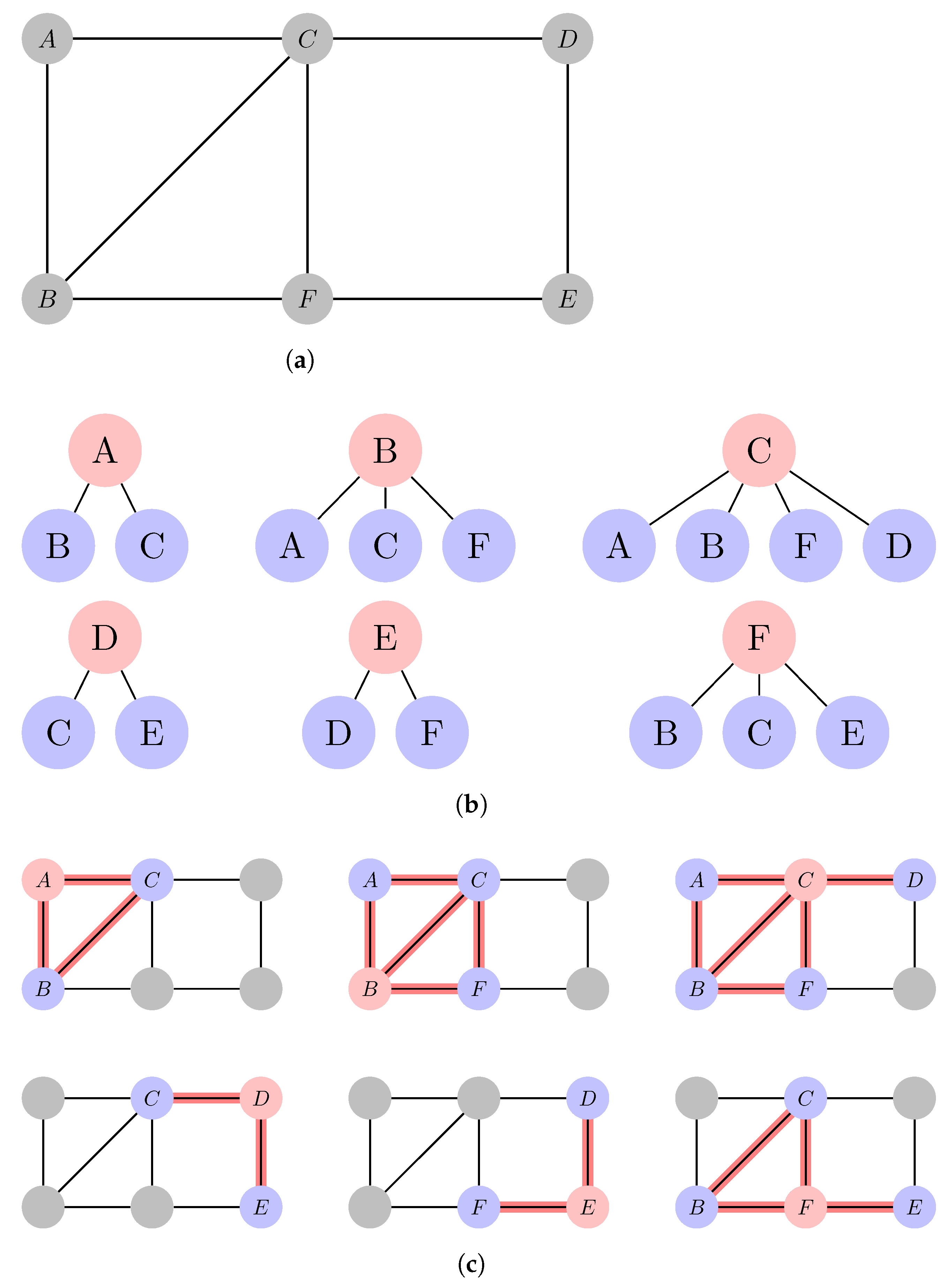
3.2. Graph Isomorphism and Weisfeiler–Leman

The problem of graph isomorphism can be formulated mathematically in the following way. Given two graphs $G_1,G_2$, they are said to be isomorphic if they have the same number of nodes and there exists a permutation that maps each node of $G_1$ to a node in $G_2$, while preserving the structure, i.e., the edges.

One famous class of algorithms used for determining if two graphs are isomorphic is the Weisfeiler–Leman (WL) algorithm, also called 1-WL [37]. It can be viewed as a graph coloring scheme. Let $c_i^{\left(t\right)}$ be the color of node i at step t. Then, the algorithm iterates according to Equation (9). For each node, it updates its color at step $t+1$ based on its color and the color of its neighbors at the previous step t using a hash function. The link between GNNs and WL was pointed out in [8]. A comprehensive review of the use of WL in machine learning is presented in [38].

$$c_v^{(t+1)}=HASH\left(\left(c_v^{\left(t\right)},\left\{\left\{c_u^{\left(t\right)}\mid u\in {\mathcal{N}}_v\right\}\right\}\right)\right)$$

(9)

While WL is known to fail at distinguishing some graphs, it performs well in most cases [39]. For this reason, it is often used as the reference when determining the expressive power of a GNN. The two concurrent works [4,5] proved that standard MPNNs, without node features, are at most as powerful as the 1-WL test. Additionally, Ref. [4] proposed the Graph Isomorphism Network (GIN) and proved that the architecture is as powerful at the 1-WL test.

The WL tests can be extended to k-WL where $k\ge 2$ [40]. Instead of coloring a single node, we color tuples of size k. Let $v_i\in V^k$ be a k-tuple of $\mathcal{G}$, i.e. $v_i=(v_{i_1},\dots ,v_{i_k})$ where $v_{i_j}\in V$ for $j\in \left[k\right]$. For the k-WL, we define the neighborhood of a tuple $v_i$ to be

$${\mathcal{N}}_j\left(v_i\right)=\left(\left\{(v_{i_1},\dots ,v_{i_{j-1}},u,v_{i_{j+1}},v_{i_k})\mid u\in V\right\}\right).$$

(10)

Similarly, for Folklore WL (k-FWL) [40], a variant of the WL algorithms that uses a different update rule, the neighborhood of $v_i$ is defined as

$${\mathcal{N}}_u^F\left(v_i\right)=\left((u,v_{i_2},\dots ,v_{i_k}),(v_{i_1},u,\dots ,v_{i_k}),\dots ,(v_{i_1},\dots ,v_{i_{k-1}},u)\right).$$

(11)

Using these neighborhoods, the update rule for k-WL follows Equation (12), while k-FWL follows Equation (13).

$$\begin{array}{cc}\hfill & c_{v_i}^{(t+1)}=HASH\left(\left(c_{v_i}^{\left(t\right)},\left\{\left\{c_u^{\left(t\right)}\mid u\in {\mathcal{N}}_j\left(v_i\right),j\in \left[k\right]\right\}\right\}\right)\right)\hfill \end{array}$$

(12)

$$\begin{array}{cc}\hfill & c_{v_i}^{(t+1)}=HASH\left(\left(c_{v_i}^{\left(t\right)},\left\{\left\{c_u^{\left(t\right)}\mid u\in {\mathcal{N}}_j^F\left(v_i\right),j\in \left[n\right]\right\}\right\}\right)\right)\hfill \end{array}$$

(13)

Since k-WL are known to be strictly more powerful than $(k-1)$-WL for $k\ge 2$, and k-WL and $(k-1)$-FWL have the same expressive power, adapting k-WL for GNNs leads to more expressive GNNs [5,6]. This leads to higher order networks and invariant networks.

4. Higher Order Networks and Universal Approximation

Building network layers that work on tuples of nodes instead of single nodes requires using tensors of higher dimension. Instead of having an input feature matrix $X\in {\mathbb{R}}^{n\times d}$ with an adjacency matrix $A\in {\{0,1\}}^{n\times n}$, a hyper-graph can be represented using a tensor $\mathsf{X}\in {\mathbb{R}}^{n^k\times d}$ [41]. In this manner, ${\mathsf{X}}_i$ represents the features of node i, ${\mathsf{x}}_{i,j}$ of edge $(i,j)$, ${\mathsf{X}}_{i,j,l}$ of the hyper edge $(i,j,l)$, and so on.

Because the ordering of the nodes is arbitrary, the GNN layers should be designed to be either permutation equivariant or invariant. A composition of an equivariant layer with an invariant layer leads to an invariant function. In [41], the authors characterize all such types of linear layers. Namely, given a permutation matrix P and a function vec that vectorizes a tensor, a linear layer $L\in {\mathbb{R}}^{1\times n^k}$ is invariant if and only if it follows Equation (14):

$$P^{⨂k}vec\left(L\right)=vec\left(L\right)$$

(14)

where $⨂$ is the Kronecker product. Similarly, a linear layer $L\in {\mathbb{R}}^{n^k\times n^k}$ is equivariant if and only if it follows Equation (15).

$$P^{⨂2k}vec\left(L\right)=vec\left(L\right)$$

(15)

The authors [41] further provide a basis for the space of invariant and equivariant layers, alongside their dimension.

Instead of trying to directly create an invariant layer, one can use arbitrary functions and sum over all the permutations. This was first proposed in [10]. Given $X_{features,id}$ the feature matrix concatenated with a one-hot encoding of a position of the node, f a GNN, a Relational Pooling GNN (RP-GNN) layer follows Equation (16). $\pi$ is a permutation of the nodes of $\mathcal{G}$. The one-hot encoding added to X is permuted with $\pi$ while X remains fixed. This prevents the sum from reducing to a single element. Furthermore, selecting the permutations on which to perform the sum can eliminate the factorial complexity induced by all the permutations.

$$f_{RP}\left(G\right)=\frac{1}{\left|\mathcal{V}\right|!}\sum _{\pi \in {\prod }_{\left|\mathcal{V}\right|}}f(\pi \left(A\right),X_{features,\pi \left(id\right)})$$

(16)

Building equivariant and invariant layers raises a question: can the network approximate any invariant or equivariant function, i.e., can GNNs act as universal approximators? Provided that the tensors have a high enough dimension, Ref. [9] proved that models based on the linear layers defined above can indeed approximate any invariant functions. Specifically, networks using layers that are equivariant or invariant for a group G can be expressed as in Equation (17):

$$\varphi =m\circ h\circ {\sigma }_l\left(L_d\right)\circ \cdots \circ {\sigma }_1\left(L_1\right)$$

(17)

where m is a multi-layer perceptron that flattens the output, h is a function that is invariant for the group G, and $L_i$ are the equivariant layers for the group G that follow Equation (15).

Similarly, in addition to providing a different proof of the result from [9] regarding the universality of the linear layers following Equation (14) with respect to invariant functions, the authors of [13] show that, given a sufficient tensor size, equivariant networks can approximate any equivariant function.

In terms of graph isomorphism, k-order GNNs, that is, GNNs that use a k-order tensor as input such as hypergraphs, are more expressive than GNNs. Specifically, they are as powerful as k-WL [6].

The problem with k-order GNNs is that they are computationally too expensive. Universality results for computationally reasonable GNNs were first proven in [42], additionally showing that Folklore GNNs are the most expressive for a given k.

To design GNNs that are more powerful than 1-WL while still being computationally efficient, we must exploit node properties such as their identification and the substructures that they belong to.

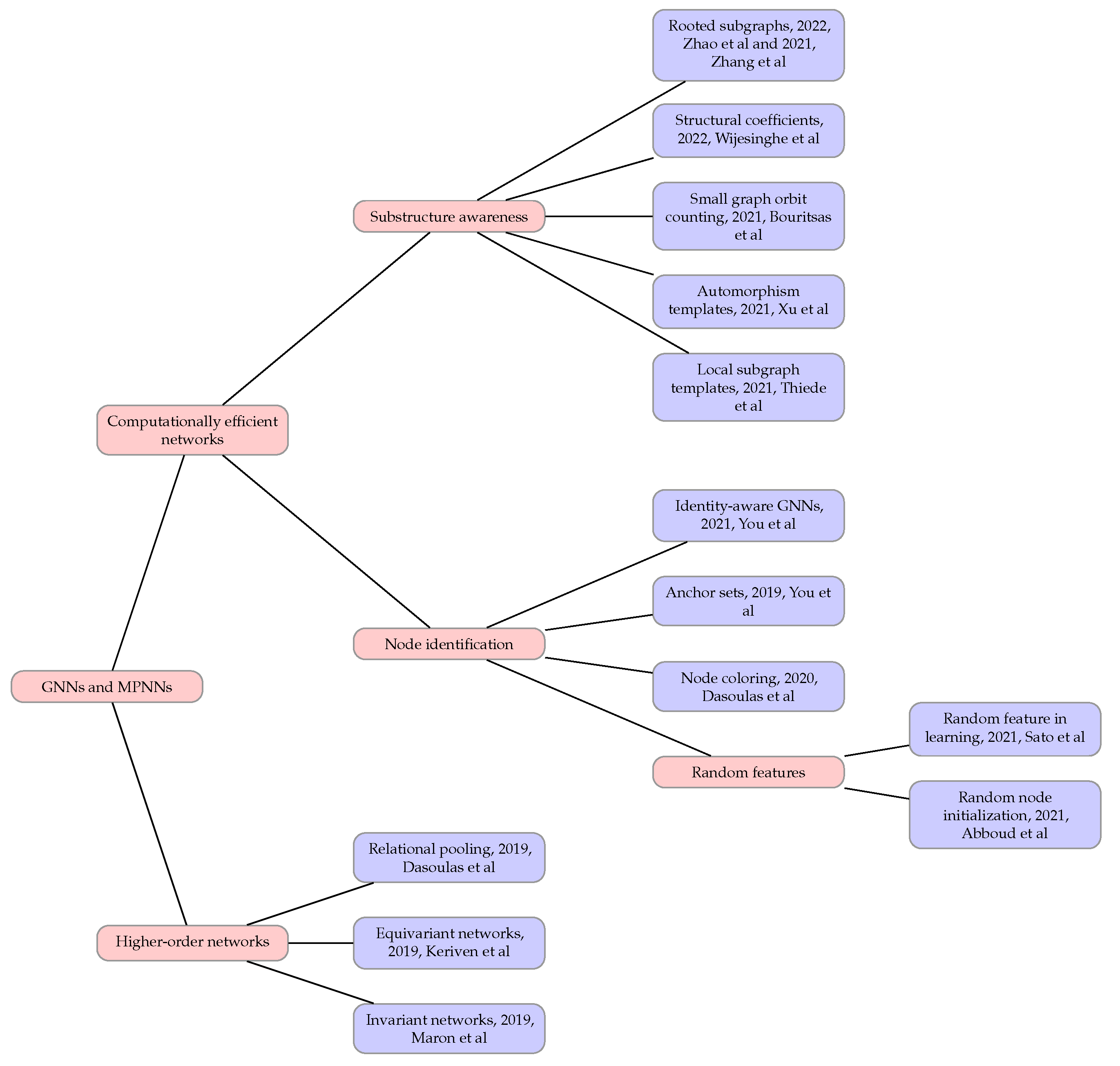
5. Computationally Efficient and Powerful Networks

Instead of using higher-order networks, finding more expressive architectures than GNNs can be done by looking at the failure cases of MPNNs. Most of the failures can be attributed to two related causes: the anonymity of nodes in the message passing stage, where it is impossible to keep track of where the information is coming from [36]; and the lack of substructure awareness from MPNNs [43].

Mitigating node anonymity is the subject of Section 5.1, while injecting substructure awareness into MPNNs is discussed in Section 5.2.

5.1. Node Identification

MPNNs cannot distinguish information coming from identical nodes (i.e., nodes with the same features and same degree). One way to remedy this problem is to color each identical node with a different color. This is the process introduced in [11] with the k-CLIP (Colored Local Iterative Procedure) algorithm. Each node with identical attributes are mapped into groups $V_1,\dots ,V_K$. Within each group, each node is assigned a distinct color, by concatenating the color attribute, e.g., a one-hot encoding, with the features of the node. k different coloring ${\mathcal{C}}_k$ are chosen out of all the possible colorings. A standard MPNN is trained for each coloring, and the final output is given by Equation (18):

$$h_G=\psi \left(\underset{c\in {\mathcal{C}}_k}{max}\sum _{v\in \mathcal{V}}{h}_{v,L}^c\right)$$

(18)

where $h_G$ is the graph readout of the network, $\psi$ is a learnable function, and $h_{v,L}^c$ is the hidden representation of node v at the last layer L of the network using the coloring c. Compared to a standard MPNN, the complexity of k-CLIP has an extra k factor that corresponds to the number of colorings used. CLIP can be used with all the ${\prod }_{k=1}^K\left|V_k\right|$ possible colorings, in which case it is named ${\infty }_{\mathrm{CLIP}}$. While the ${\infty }_{\mathrm{CLIP}}$ is a universal approximator [11], it suffers from an exponential growth with respect to the size of the $V_k,k\in \left[K\right]$. k-CLIP is a random algorithm, e.g., two different runs might lead to two different colorings. It is more efficient than ${\infty }_{\mathrm{CLIP}}$, and universality results can still be obtained for its expectancy [11].

When a GNN has a sufficient number of layers, a node is feeding back information to itself in its update: in an undirected graph, a node is a neighbor of its neighbor. For example, given the graph in Figure 2a and the trees of height 1 starting from each of its nodes in Figure 2b, B is a neighbor of A. With a standard MPNN, A will be used to update B, which in turn will be used to update A, with no indication of the provenance of the information. Therefore, as shown in [19], graphs with different structures can have the same GNN computational graph. To alleviate this problem, the authors propose to introduce identity-aware GNNs (ID-GNNs), where they use ego networks (rooted graphs) in which the root is colored and thus can be identified in the computational graph. Figure 2c shows the ego networks of height 1 for each of the nodes in the graph of Figure 2a. An ID-GNN layer follows Equations (19) and (20), where $MESSAG{E}_0$ and $MESSAG{E}_1$ can be MLPs, attention mechanisms, etc. $MESSAG{E}_0$ is the message function for neighbors of the root node, while $MESSAG{E}_1$ is the message function to update the root node. This set of equations are similar to Equations (4) and (5), except that the root node of the ego graphs is identified and its message is used differently than for the rest of the nodes. There is almost no added complexity compared to a standard MPNN: by setting $MESSAG{E}_0=MESSAG{E}_1$, we recover a standard MPNN. However, ID-GNNs can differentiate graphs that a Graph Isomorphism Network [4] cannot, making them strictly more powerful than the 1-WL test [19].

$$\begin{array}{cc}\hfill & m_v^{(l+1)}=AGGREGATE\left(\left\{\left\{MESSAG{E}_0\left(h_u^{\left(l\right)}\right)\mid u\in {\mathcal{N}}_v\right\}\right\}\right)\hfill \end{array}$$

(19)

$$\begin{array}{cc}\hfill & h_v^{(l+1)}=UPDATE\left(MESSAG{E}_1\left(h_v^{\left(l\right)}\right),m_v^{(l+1)}\right)\hfill \end{array}$$

(20)

A simpler approach consists in simply assigning a random feature to each node at the beginning of the learning phase. Namely, the node feature matrix X is concatenated with a matrix $R\in {\mathbb{R}}^{N\times d_r}$ where R is a feature matrix that was sampled from a random distribution. rGIN, the architecture obtained by adding the random feature assignment to a standard GIN, can distinguish graphs that GIN cannot [21]. The random features ensure that graphs that lead to the same GNN computational graphs will produce different graphs most of the time with randomization. Additionally, random node initialization allows MPNNs to become universal approximators without requiring higher order tensors [22].

Instead of using the neighborhood of each node, one can use anchor sets, which consist of nodes sampled from the graphs. In [20], the authors propose the Position-aware Graph Neural Network. At each layer, k sets $S_i,i\in \left[k\right]$ of nodes are chosen. Then, for each node v, a message $m_{v,i}$ is computed between v and the nodes in $S_i$, as in Equation (21). Finally, the hidden representation is updated by aggregating the messages from all the anchor sets, as shown in Equation (22).

$$m_{v,i}^{\left(l\right)}=AGGREGATE\left(\left\{\left\{h_u^{\left(l\right)}\mid u\in S_i\right\}\right\}\right)$$

(21)

$$h_v^{(l+1)}=AGGREGATE\left(\left\{\left\{m_{v,i}^{\left(l\right)}\mid i\in \left[k\right]\right\}\right\}\right)$$

(22)

Removing the dependency on the neighborhood of the nodes changes the objective function of the network. Following [20], the representation learning objective of a GNN is written in Equation (23). $\varphi$ represents the neural network parameterized by $\theta$. Nodes u and v are sampled according to ${\mathcal{V}}_{train}$, the distribution of nodes in the training set. $S_u$ is the q-hop neighborhood graph of u, parameterized by q, the maximum distance to u. $S_u$ and $S_v$ are sampled according to $p\left(\mathcal{V}\right)$, the distribution of the set of nodes in the graph. $d_z$ is a similarity metric, and $d_y$ is a target similarity metric. By contrast, the learning objective of a P-GNN is written in Equation (24), where S is an anchor set, sampled from the distribution $p\left(\mathcal{V}\right)$. P-GNN can share information across the whole graph using common anchors between nodes, while a standard GNN is restricted to the nodes in the neighborhood. This makes P-GNN able to approximately capture properties that GNNs cannot capture, such as the shortest paths in the network.

$$\underset{\theta }{min}\mathbb{E}\left[\mathcal{L}(d_z({\varphi }_{\theta }(u,S_u),{\varphi }_{\theta }(v,S_v))-d_y(u,v))\right]$$

(23)

$$\underset{\theta }{min}\mathbb{E}\left[\mathcal{L}(d_z({\varphi }_{\theta }(u,S),{\varphi }_{\theta }(v,S))-d_y(u,v))\right]$$

(24)

In place of identifying each node, the expressiveness of MPNNs can also be improved by making them aware of the substructures found in the graph.

5.2. Substructure Awareness

One area of interest is whether MPNNs can count substructures. That is, given a graph structure or pattern, can an MPNN count the number of times that such structure, up to isomorphisms, appear in the graph? The authors of [43] show that MPNNs cannot count patterns with three or more nodes. However, MPNNs can perform subgraph-count of star-shaped patterns. Looking at k-WL tests, the authors further show that finite k-WL cannot perform an induced-subgraph-count of patterns that have more than a given number of nodes.

MPNNs rely on a star-shaped aggregation pattern: they aggregate information coming from neighbors to a central node (see Equation (1)). For example, in Figure 2a, node C and E are treated in the same way to update node F. However, C and E do not have the same structural information, as C is part of a triangle with B and F, while E forms one of the endpoints of a path of length 2 with F. To capture this information, Ref. [12] proposes the Autobahn architecture. Given a list of template graphs, at each layer, the network decomposes the graph into a collection of subgraphs that are isomorphic to the templates. A single neuron in the Autobahn is applied to subgraphs that match the list of templates. The activation from the different templates are combined using narrowing and promotion functions that allow us to, respectively, extend or decrease the number of nodes that an activation function takes. The authors [12] argue that if the templates are carefully chosen, Autobahn can match the expressiveness of higher order networks.

In a similar work, the authors of [18] propose the GRaph AutomorPhic Equivalence (GRAPE) network, which uses automorphism groups in a similar manner to Autobahn [12]. They focus on template search using genetic algorithms: templates are produced from a pool, and mutated via edge mutation or node mutation until a satisfactory template has been produced. The authors [18] further show that GRAPE can distinguish certain graphs that MPNNs cannot distinguish.

By contrast, in [17], the authors propose to use a list of small connected graphs to directly add structural features to nodes and edges by counting the number of times a node (or an edge) acts as a member of an orbit of one the graphs. For example, in Figure 2c, node C acts as a point in a triangle for the A rooted graph, but as one end of a path of length 3 in the D rooted path. The structural features can be concatenated with the original features and a GNN is trained on the new features. The authors [17] show that under certain conditions on the subgraph matching, this type of architecture, called Graph Substructure Networks (GSN), can be strictly more powerful than MPNNs and 1-WL.

On the topic of substructures, a new hierarchy of local isomorphisms between subgraphs is proposed in [16]: subgraph isomorphism, overlap isomorphism and subtree isomorphism. Let $S_u$ be the neighborhood subgraph of u. It is the subgraph induced by ${\tilde{\mathcal{N}}}_u={\mathcal{N}}_u\cup u$. The overlap subgraph between two adjacent vertices u and v is defined by $S_{uv}=S_u\cap S_v$. Let $\mathcal{S}=\left\{S_v\right|v\in \mathcal{V}\}$ and ${\mathcal{S}}^{*}=\left\{S_{vu}\right|(v,u)\in \mathcal{E}\}$. Structural coefficients for nodes and their neighbors can be obtained by defining a function $\omega \in \mathcal{S}\times {\mathcal{S}}^{*}\to \mathbb{R}$ that have the following properties: (1) local closeness: $\omega (S_v,S_{vu})>\omega (S_v,S_{v{u}^{\prime }})$ if $S_{vu}$ and $S_{v{u}^{\prime }}$ are complete graphs and $S_{vu}$ has more vertices than $S_{v{u}^{\prime }}$; (2) local denseness: $\omega (S_v,S_{vu})>\omega (S_v,S_{v{u}^{\prime }})$ if $S_{vu}$ and $S_{u{v}^{\prime }}$ have the same number of vertices, but $S_{vu}$ has more edges; (3) isomorphic invariant: $\omega (S_v,S_{vu})>\omega (S_v,S_{v{u}^{\prime }})$ if $S_{vu}$ and $S_{v{u}^{\prime }}$ are isomorphic.

Based on these criteria, the authors in [16] propose the GraphSNN architecture. It follows Equations (25)–(27). Equation (28) is an example of a valid $\omega$ function, parameterized by $\lambda >0$. $|{\mathcal{V}}_{vu}|$ is the number of vertices of $S_{u}v$, and $|{\mathcal{E}}_{vu}|$ its number of edges. Furthermore, the $\omega (S_v,S_{vu})$ can be normalized for the network operations. With this $\omega$, GraphSNN is more powerful than 1-WL [16].

$$\begin{array}{ll}& m_a^{\left(l\right)}=AGGREGAT{E}_0\left(\left\{\left\{\left(\omega (S_v,S_{vu}),h_u^{\left(l\right)}\right)\mid u\in {\mathcal{N}}_v\right\}\right\}\right)\end{array}$$

(25)

$$\begin{array}{ll}& m_v^{\left(l\right)}=AGGREGAT{E}_1\left(\left\{\left\{\left(\omega (S_v,S_{vu}\right)\mid u\in {\mathcal{N}}_v\right\}\right\}\right)h_v^{\left(l\right)}\end{array}$$

(26)

$$\begin{array}{ll}& h_v^{(l+1)}=UPDATE(m_a^{\left(l\right)},m_v^{\left(l\right)})\end{array}$$

(27)

$$\begin{array}{ll}& \omega (S_v,S_{vu})=\frac{|{\mathcal{E}}_{vu}|}{|{\mathcal{V}}_{vu}|·|{\mathcal{V}}_{vu}-1|}{\left|{\mathcal{V}}_{vu}\right|}^{\lambda }\end{array}$$

(28)

Alternatively, instead of relying on structural coefficients or graph templates, we can exploit the rooted subgraphs of each node. In this setting, we employ a network uplifting scheme where a base GNN is used to compute node representations, which are fed to an outer GNN. In [14], the authors use rooted graphs to compute three types of information: the centroid encoding, which is obtained when the node is the root of the rooted graph; the subgraph encoding, which represents the information from the other nodes in the rooted graph; and the context encoding, which represents the information that the node carries in the other rooted graphs. Let $G^{\left(l\right)}\left[{\mathcal{N}}_k\left(v\right)\right]$ be the v rooted graph with height k, with the node representations from layer l. Let $GN{N}^{\left(l\right)}=POO{L}_{GN{N}^{\left(l\right)}}\left(EM{B}^{\left(l\right)}\left(i\right|G^{\left(l\right)}\left[{\mathcal{N}}_k\left(v\right)\right])\right|i\in {\mathcal{N}}_k\left(v\right))$ be the inner GNN, with $POO{L}_{GN{N}^{\left(l\right)}}$ the pooling operator after the last layer of the GNN, and $EM{B}^{\left(l\right)}\left(i\right|G^{\left(l\right)})$ the embeddings before the pooling operation of the GNN. Let $d_{u|v}^{\left(l\right)}$ be the encoding of distance from node u to v at layer l [44]. Let $\sigma$ be the sigmoid function, ⊙ the element-wise product. The GNN As Kernel (GNN-AK) architecture follows Equations (29)–(32). The authors [14] prove that this GNN-AK is strictly more powerful than 2-WL and not less powerful than 3-WL.

$$\begin{array}{cc}\hfill & h_{v,subgraph}^{(l+1)}=POO{L}_{GNN}\left(\left\{\left(\sigma \left(d_{u|v}^{\left(l\right)}\right)\odot EMB\left(i\mid G^{\left(l\right)}\left[{\mathcal{N}}_k\left(v\right)\right]\right)\right),i\in {\mathcal{N}}_k\left(v\right)\right\}\right)\hfill \end{array}$$

(29)

$$\begin{array}{cc}\hfill & h_{v,centroid}^{(l+1)}=EMB\left(v\mid G^{(l+1)}\left[{\mathcal{N}}_k\left(v\right)\right]\right)\hfill \end{array}$$

(30)

$$\begin{array}{cc}\hfill & h_{v,context}^{(l+1)}=POO{L}_{CONTEXT}\left(\left\{\left(\sigma \left(d_{u|v}^{\left(l\right)}\right)\odot EMB\left(v\mid G^{\left(l\right)}\left[{\mathcal{N}}_k\left(u\right)\right]\right)\right),v\in {\mathcal{N}}_k\left(u\right)\right\}\right)\hfill \end{array}$$

(31)

$$\begin{array}{cc}\hfill & h_v^{(l+1)}=UPDATE\left(h_{v,subgraph}^{(l+1)},h_{v,centroid}^{(l+1)},h_{v,context}^{(l+1)}\right)\hfill \end{array}$$

(32)

WL and MPNNs encode a rooted subtree for each node. This is illustrated in Figure 2a,b. The nodes in red in Figure 2b are updated using information from the nodes in blue. Information about edges between the nodes in blue is lost. This might prevent the network from learning useful information at the graph level. Instead, Ref. [15] proposes to learn subgraph representations centered around rooted graphs. Let $G_v^h$ be be the rooted graph of v with height h, and $\mathcal{N}\left(v\right|G_w^h)$ the neighborhood of v within w’s rooted subgraph. A layer of Nested Graph Neural Network (NGNN) follows Equations (33) and (34). In the last layer, the representation of node w is obtained by performing a readout, as shown in Equation (35) where L is the last layer and $R_0$ is the readout function. These new representations can be used as an input to a second GNN to perform graph-level tasks. These nested architectures are strictly more powerful than 1-WL [15].

$$\begin{array}{cc}\hfill & m_{v,G_w^h}^{(l+1)}=AGGREGATE\left(\left\{\left\{h_{u,G_w^h}^{\left(l\right)}\mid u\in \mathcal{N}(v\mid G_w^h\right\}\right\}\right)\hfill \end{array}$$

(33)

$$\begin{array}{cc}\hfill & h_{v,G_w^h}^{\left(l\right)}=UPDATE\left(h_{v,G_w^h}^{\left(l\right)},m_{v,G_w^h}^{(l+1)}\right)\hfill \end{array}$$

(34)

$$\begin{array}{cc}\hfill & h_w=R_0\left(h_{v,G_w^h}^L\mid v\in G_w^h\right)\hfill \end{array}$$

(35)

While graphs may be difficult to distinguish, it is usually easier to distinguish subgraphs. With this in mind, Ref. [45] propose using bags of subgraphs that can then be readout, and on which a set operation can be performed. There can be different policies in selecting the subgraphs. These methods are more powerful than 1-WL.

6. Summary

The early works regarding GNN expressiveness were focused on two goals: providing bounds for MPNNs, and overcoming those bounds. The works of [4,5] established Weisfeiler–Leman tests as the standard of comparison when it comes to expressiveness of GNNs. The higher-order Weisfeiler–Leman tests provide a template for higher-order GNNs [40].

Higher-order methods also arise when trying to design GNN layers that are universal approximators or invariant [9] or equivariant functions [13]. To this end, hypergraphs with tensors containing hyperedges data are required [41].

With higher-order networks, the complexity grows exponentially with the number of nodes. This makes these networks computationally expensive, and alternatives must be crafted to handle large graphs. Approaches with low overhead compared to a standard MPNNs include some form of node identification. This can be achieved by adding colors to each node [11], using rooted graphs [19], fixing sets of nodes that are used to update all the nodes in the graph [20], or by adding random features to the nodes [21,22].

To retain part of the expressiveness of higher-order networks, subgraphs can be used as templates on which to perform the convolutions. This breaks the star-shaped pattern of MPNN convolutions and allows for other patterns such as triangles, circles, etc. A network with a good selection of templates can be viewed as a higher-order network where only a few substructures are used [12]. These templates can be searched via genetic algorithms [18].

Substructures can also be used to add structural information to the nodes. This can be achieved by counting the roles a node plays in different templates and adding this information to the features [17]. Alternatively, structural coefficients which take into account the shapes of neighborhoods can inject structural information into the network [16].

On top of the previous methods, GNNs can be used a building block for other GNNs. An inner GNN using rooted graphs can be used to produce hidden representations that are fed into an outer GNN [15]. Moreover, each node can be updated using three types of information: the centroid information, when the node is the root of the rooted graph; the subgraph information, which is the information coming from its neighbors; and the context information, which is the information it contributes to rooted graphs where it is not the root [14].

All the expressiveness results of the architectures discussed in the paper are presented in

Table 2. Expressiveness of GNNs. Expressiveness is given with respect to how the authors proved the results. GIN corresponds to the most powerful standard MPNN.

Architecture	Expressiveness
GIN [4]	1-WL
k-GNN [5]	(k-1)-WL
RP-GNN [10]	strictly superior to GIN
PPGN [6]	3-WL
${\infty }_{CLIP}$ [11]	universal approximator
ID-GNN [19]	>1-WL
rGIN [21]	>1-WL, universal approximator
PGNN [20]	greater than MPNN
Autobahn [12]	depends on the templates, can achieve k-GNN performance
GRAPE [18]	stricly more powerful than MPNN
GSN [17]	more powerful than MPNN and 1-WL under conditions.
GraphSNN [16]	$>1\mathrm{-WL}$
GNN-AK [14]	>2-WL, ≥ 3-WL
NGNN [15]	> 1-WL

. The table contains only results that have a mathematical proof in the associated paper. In some cases, this could mean that higher bounds can exist that have not been proven. Conversely, new architectures that are developed today could have a high expressiveness, but since no mathematical proof is provided, the evidence is only empirical.

7. Conclusions and Future Works

In this survey, we present the expressive properties of standard graph neural networks. We detail the two main ways in which we can improve the expressiveness of the models. On the one hand, we can achieve maximally expressive networks by using higher order networks that rely on hypergraph data and averaging over all node permutations, which is computationally expensive. On the other hand, incorporating substructure awareness or node identification in standard GNNs can also improve expressiveness while remaining computationally efficient compared to higher order methods.

To the best of our knowledge, there has yet been no papers investigating the expressive power of methods that combine the methods presented in Section 5. For example, can the gains made in mathematical expressiveness from adding node identifiers be combined with the ones made from using nested graph neural networks? Or do these gains have the same root, rendering the combination as powerful as either of the methods individually?

Another way to improve expressiveness is to extend GNNs to more complex structures such as cell complexes, of which graphs are special cases [46]. Graphs can be seen as part of a bigger framework of geometric objects, which can be worked on using geometric deep learning [33]. A possible line of work would be to explore other types of structures that share profound links with graphs, and create efficient architectures that can be adapted to graphs.

References

1. Scarselli, F.; Gori, M.; Tsoi, A.C.; Hagenbuchner, M.; Monfardini, G. The Graph Neural Network Model. IEEE Trans. Neural Netw. 2009, 20, 61–80. [Google Scholar] [CrossRef] [PubMed] [Green Version]
2. Zhou, J.; Cui, G.; Hu, S.; Zhang, Z.; Yang, C.; Liu, Z.; Wang, L.; Li, C.; Sun, M. Graph Neural Networks: A Review of Methods and Applications. AI Open 2020, 1, 57–81. [Google Scholar] [CrossRef]
3. Gilmer, J.; Schoenholz, S.S.; Riley, P.F.; Vinyals, O.; Dahl, G.E. Neural Message Passing for Quantum Chemistry. In Proceedings of the 34th International Conference on Machine Learning, ICML 2017, Sydney, NSW, Australia, 6–11 August 2017; Volume 70, pp. 1263–1272. [Google Scholar]
4. Xu, K.; Hu, W.; Leskovec, J.; Jegelka, S. How Powerful Are Graph Neural Networks? In Proceedings of the 7th International Conference on Learning Representations, ICLR 2019, New Orleans, LA, USA, 6–9 May 2019.
5. Morris, C.; Ritzert, M.; Fey, M.; Hamilton, W.L.; Lenssen, J.E.; Rattan, G.; Grohe, M. Weisfeiler and Leman Go Neural: Higher-Order Graph Neural Networks. In Proceedings of the AAAI Conference on Artificial Intelligence, Honolulu, HI, USA, 27 January–1 February 2019; Volume 33, pp. 4602–4609. [Google Scholar] [CrossRef] [Green Version]
6. Maron, H.; Ben-Hamu, H.; Serviansky, H.; Lipman, Y. Provably Powerful Graph Networks. In Proceedings of the Advances in Neural Information Processing Systems 32: Annual Conference on Neural Information Processing Systems 2019, NeurIPS 2019, Vancouver, BC, Canada, 8–14 December 2019; pp. 2153–2164. [Google Scholar]
7. Barceló, P.; Kostylev, E.V.; Monet, M.; Pérez, J.; Reutter, J.L.; Silva, J.P. The Logical Expressiveness of Graph Neural Networks. In Proceedings of the 8th International Conference on Learning Representations, ICLR 2020, Addis Ababa, Ethiopia, 26–30 April 2020. [Google Scholar]
8. Kipf, T.N.; Welling, M. Semi-Supervised Classification with Graph Convolutional Networks. In Proceedings of the 5th International Conference on Learning Representations, ICLR 2017, Toulon, France, 24–26 April 2017. [Google Scholar]
9. Maron, H.; Fetaya, E.; Segol, N.; Lipman, Y. On the Universality of Invariant Networks. In Proceedings of the 36th International Conference on Machine Learning, ICML 2019, Long Beach, CA, USA, 9–15 June 2019; Volume 97, pp. 4363–4371. [Google Scholar]
10. Murphy, R.L.; Srinivasan, B.; Rao, V.A.; Ribeiro, B. Relational Pooling for Graph Representations. In Proceedings of the 36th International Conference on Machine Learning, ICML 2019, Long Beach, CA, USA, 9–15 June 2019; Volume 97, pp. 4663–4673. [Google Scholar]
11. Dasoulas, G.; Santos, L.D.; Scaman, K.; Virmaux, A. Coloring Graph Neural Networks for Node Disambiguation. In Proceedings of the Twenty-Ninth International Joint Conference on Artificial Intelligence, IJCAI 2020, Yokohama, Japan, 7–15 January 2021; pp. 2126–2132. [Google Scholar] [CrossRef]
12. Thiede, E.H.; Zhou, W.; Kondor, R. Autobahn: Automorphism-based Graph Neural Nets. In Proceedings of the Advances in Neural Information Processing Systems 34: Annual Conference on Neural Information Processing Systems 2021, NeurIPS 2021, Virtual, 6–14 December 2021; pp. 29922–29934. [Google Scholar]
13. Keriven, N.; Peyré, G. Universal Invariant and Equivariant Graph Neural Networks. In Proceedings of the Advances in Neural Information Processing Systems 32: Annual Conference on Neural Information Processing Systems 2019, NeurIPS 2019, Vancouver, BC, Canada, 8–14 December 2019; pp. 7090–7099. [Google Scholar]
14. Zhao, L.; Jin, W.; Akoglu, L.; Shah, N. From Stars to Subgraphs: Uplifting Any GNN with Local Structure Awareness. In Proceedings of the Tenth International Conference on Learning Representations, ICLR 2022, Virtual Event, 25–29 April 2022. [Google Scholar]
15. Zhang, M.; Li, P. Nested Graph Neural Networks. In Proceedings of the Advances in Neural Information Processing Systems 34: Annual Conference on Neural Information Processing Systems 2021, NeurIPS 2021, Virtual, 6–14 December 2021; pp. 15734–15747. [Google Scholar]
16. Wijesinghe, A.; Wang, Q. A New Perspective on “How Graph Neural Networks Go Beyond Weisfeiler-Lehman?”. In Proceedings of the Tenth International Conference on Learning Representations, ICLR 2022, Virtual Event, 25–29 April 2022. [Google Scholar]
17. Bouritsas, G.; Frasca, F.; Zafeiriou, S.; Bronstein, M.M. Improving Graph Neural Network Expressivity via Subgraph Isomorphism Counting. arXiv 2021, arXiv:2006.09252. [Google Scholar] [CrossRef] [PubMed]
18. Xu, F.; Yao, Q.; Hui, P.; Li, Y. Automorphic Equivalence-Aware Graph Neural Network. In Proceedings of the Advances in Neural Information Processing Systems 34: Annual Conference on Neural Information Processing Systems 2021, NeurIPS 2021, Virtual, 6–14 December 2021; pp. 15138–15150. [Google Scholar]
19. You, J.; Selman, J.M.G.; Ying, R.; Leskovec, J. Identity-Aware Graph Neural Networks. In Proceedings of the Thirty-Fifth AAAI Conference on Artificial Intelligence, AAAI 2021, Thirty-Third Conference on Innovative Applications of Artificial Intelligence, IAAI 2021, the Eleventh Symposium on Educational Advances in Artificial Intelligence, EAAI 2021, Virtual Event, 2–9 February 2021; pp. 10737–10745. [Google Scholar]
20. You, J.; Ying, R.; Leskovec, J. Position-Aware Graph Neural Networks. In Proceedings of the 36th International Conference on Machine Learning, ICML 2019, Long Beach, CA, USA, 9–15 June 2019; Volume 97, pp. 7134–7143. [Google Scholar]
21. Sato, R.; Yamada, M.; Kashima, H. Random Features Strengthen Graph Neural Networks. In Proceedings of the 2021 SIAM International Conference on Data Mining, SDM 2021, Virtual Event, 29 April–1 May 2021; pp. 333–341. [Google Scholar] [CrossRef]
22. Abboud, R.; Ceylan, İ.İ.; Grohe, M.; Lukasiewicz, T. The Surprising Power of Graph Neural Networks with Random Node Initialization. In Proceedings of the Thirtieth International Joint Conference on Artificial Intelligence, IJCAI 2021, Virtual Event, 19–27 August 2021; pp. 2112–2118. [Google Scholar] [CrossRef]
23. Ma, Y.; Tang, J. Deep Learning on Graphs; Cambridge University Press: Cambridge, UK, 2021. [Google Scholar]
24. Velickovic, P.; Cucurull, G.; Casanova, A.; Romero, A.; Liò, P.; Bengio, Y. Graph Attention Networks. In Proceedings of the 6th International Conference on Learning Representations, ICLR 2018, Vancouver, BC, Canada, 30 April–3 May 2018. [Google Scholar]
25. Hamilton, W.L.; Ying, R.; Leskovec, J. Inductive Representation Learning on Large Graphs. In Proceedings of the 31st International Conference on Neural Information Processing Systems, Long Beach, CA, USA, 4–9 December 2017; Curran Associates Inc.: Red Hook, NY, USA, 2017; pp. 1025–1035. [Google Scholar]
26. Battaglia, P.W.; Hamrick, J.B.; Bapst, V.; Sanchez-Gonzalez, A.; Zambaldi, V.; Malinowski, M.; Tacchetti, A.; Raposo, D.; Santoro, A.; Faulkner, R.; et al. Relational Inductive Biases, Deep Learning, and Graph Networks. arXiv 2018, arXiv:1806.01261. [Google Scholar]
27. Bruna, J.; Zaremba, W.; Szlam, A.; LeCun, Y. Spectral Networks and Locally Connected Networks on Graphs. In Proceedings of the 2nd International Conference on Learning Representations, ICLR 2014, Banff, AB, Canada, 14–16 April 2014. [Google Scholar]
28. Defferrard, M.; Bresson, X.; Vandergheynst, P. Convolutional Neural Networks on Graphs with Fast Localized Spectral Filtering. In Proceedings of the 30th International Conference on Neural Information Processing Systems, Barcelona, Spain, 5–10 December 2016; pp. 3844–3852. [Google Scholar]
29. Wu, F.; de Souza, A.H., Jr.; Zhang, T.; Fifty, C.; Yu, T.; Weinberger, K.Q. Simplifying Graph Convolutional Networks. In Proceedings of the 36th International Conference on Machine Learning, ICML 2019, Long Beach, CA, USA, 9–15 June 2019; Volume 97, pp. 6861–6871. [Google Scholar]
30. Balcilar, M.; Renton, G.; Héroux, P.; Gaüzère, B.; Adam, S.; Honeine, P. Analyzing the Expressive Power of Graph Neural Networks in a Spectral Perspective. In Proceedings of the 9th International Conference on Learning Representations, ICLR 2021, Virtual Event, 3–7 May 2021. [Google Scholar]
31. Wu, Z.; Pan, S.; Chen, F.; Long, G.; Zhang, C.; Yu, P.S. A Comprehensive Survey on Graph Neural Networks. IEEE Trans. Neural Netw. Learn. Syst. 2021, 32, 4–24. [Google Scholar] [CrossRef] [PubMed] [Green Version]
32. Zhang, Z.; Cui, P.; Zhu, W. Deep Learning on Graphs: A Survey. IEEE Trans. Knowl. Data Eng. 2022, 34, 249–270. [Google Scholar] [CrossRef] [Green Version]
33. Bronstein, M.M.; Bruna, J.; Cohen, T.; Veličković, P. Geometric Deep Learning: Grids, Groups, Graphs, Geodesics, and Gauges. arXiv 2021, arXiv:2104.13478. [Google Scholar]
34. Dwivedi, V.P.; Joshi, C.K.; Laurent, T.; Bengio, Y.; Bresson, X. Benchmarking Graph Neural Networks. arXiv 2020, arXiv:2003.00982. [Google Scholar]
35. Chen, L.; Chen, Z.; Bruna, J. On Graph Neural Networks versus Graph-Augmented MLPs. In Proceedings of the 9th International Conference on Learning Representations, ICLR 2021, Virtual Event, 3–7 May 2021. [Google Scholar]
36. Loukas, A. What Graph Neural Networks Cannot Learn: Depth vs Width. In Proceedings of the 8th International Conference on Learning Representations, ICLR 2020, Addis Ababa, Ethiopia, 26–30 April 2020. [Google Scholar]
37. Weisfeiler, B.Y.; Leman, A.A. The reduction of a graph to canonical form and the algebra which appears therein. NTI Ser. 1968, 2, 12–16. [Google Scholar]
38. Morris, C.; Lipman, Y.; Maron, H.; Rieck, B.; Kriege, N.M.; Grohe, M.; Fey, M.; Borgwardt, K. Weisfeiler and Leman Go Machine Learning: The Story so Far. arXiv 2021, arXiv:2112.09992. [Google Scholar]
39. Cai, J.Y.; Fürer, M.; Immerman, N. An Optimal Lower Bound on the Number of Variables for Graph Identification. Combinatorica 1992, 12, 389–410. [Google Scholar] [CrossRef]
40. Douglas, B.L. The Weisfeiler-Lehman Method and Graph Isomorphism Testing. arXiv 2011, arXiv:1101.5211. [Google Scholar]
41. Maron, H.; Ben-Hamu, H.; Shamir, N.; Lipman, Y. Invariant and Equivariant Graph Networks. In Proceedings of the 7th International Conference on Learning Representations, ICLR 2019, New Orleans, LA, USA, 6–9 May 2019. [Google Scholar]
42. Azizian, W.; Lelarge, M. Expressive Power of Invariant and Equivariant Graph Neural Networks. In Proceedings of the 9th International Conference on Learning Representations, ICLR 2021, Virtual Event, 3–7 May 2021. [Google Scholar]
43. Chen, Z.; Chen, L.; Villar, S.; Bruna, J. Can Graph Neural Networks Count Substructures? In Proceedings of the Advances in Neural Information Processing Systems 33: Annual Conference on Neural Information Processing Systems 2020, NeurIPS 2020, Virtual, 6–12 December 2020.
44. Li, P.; Wang, Y.; Wang, H.; Leskovec, J. Distance Encoding: Design Provably More Powerful Neural Networks for Graph Representation Learning. In Proceedings of the Advances in Neural Information Processing Systems 33: Annual Conference on Neural Information Processing Systems 2020, NeurIPS 2020, Virtual, 6–12 December 2020. [Google Scholar]
45. Bevilacqua, B.; Frasca, F.; Lim, D.; Srinivasan, B.; Cai, C.; Balamurugan, G.; Bronstein, M.M.; Maron, H. Equivariant Subgraph Aggregation Networks. In Proceedings of the Tenth International Conference on Learning Representations, ICLR 2022, Virtual Event, 25–29 April 2022. [Google Scholar]
46. Bodnar, C.; Frasca, F.; Otter, N.; Wang, Y.; Liò, P.; Montúfar, G.F.; Bronstein, M.M. Weisfeiler and Lehman Go Cellular: CW Networks. In Proceedings of the Advances in Neural Information Processing Systems 34: Annual Conference on Neural Information Processing Systems 2021, NeurIPS 2021, Virtual, 6–14 December 2021; pp. 2625–2640. [Google Scholar]
Figure 1. Overview of mathematically expressive GNNs. Red boxes refer to sections of the paper; and blue boxes represent ideas introduced by specific papers [9,10,11,12,13,14,15,16,17,18,19,20,21,22].
Mathematics 10 04770 g001
Figure 2. Example of a graph with its rooted trees and rooted subgraphs. The rooted subgraphs incorporate structural information that is lost in rooted trees. MPNNs use rooted trees to update notes. If the features are identical, MPNNs with a single layer will treat nodes B and F as the same; if the network uses the rooted graph instead, it will distinguish B and F. (a) A graph with 6 nodes. A, D, and E have degree 2, B and F have degree 3 and F has degree 4. (b) Rooted trees with depth 1 for each node. If the nodes have identical features and are not identified, the computational tree of MPNN for A, D, and E are the same. (c) Rooted subgraphs with depth 1 for each node. Compared with the routed trees, the A rooted graph is distinguishable from D.
Mathematics 10 04770 g002