
Deep Learning Research Directions in Medical Imaging


Faculty of Computer Science, Alexandru Ioan Cuza University, 700483 Iasi, Romania
*
Author to whom correspondence should be addressed.
Mathematics 2022, 10(23), 4472; https://doi.org/10.3390/math10234472
Submission received: 29 September 2022
/
Revised: 6 November 2022
/
Accepted: 23 November 2022
/
Published: 27 November 2022
(This article belongs to the Special Issue Application of Advanced Computing and Artificial Intelligence in Engineering and Science)
Abstract
:In recent years, deep learning has been successfully applied to medical image analysis and provided assistance to medical professionals. Machine learning is being used to offer diagnosis suggestions, identify regions of interest in images, or augment data to remove noise. Training models for such tasks require a large amount of labeled data. It is often difficult to procure such data due to the fact that these requires experts to manually label them, in addition to the privacy and legal concerns that limiting their collection. Due to this, creating self-supervision learning methods and domain-adaptation techniques dedicated to this domain is essential. This paper reviews concepts from the field of deep learning and how they have been applied to medical image analysis. We also review the current state of self-supervised learning methods and their applications to medical images. In doing so, we will also present the resource ecosystem of researchers in this field, such as datasets, evaluation methodologies, and benchmarks.
Keywords:
deep learning; medical image analysis; self-supervised learning; diagnosis; brain cancer; tuberculosis; Alzheimer’s diseaseMSC:
68T071. Introduction
As humanity moves into the digital era in which digital technology becomes integrated into every aspect of our lives, the medical field has been no exception. Powered by the crossover of multiple emergent technologies such as big data processing, cloud infrastructures, deep learning, and GPU computing, medical applications for machine learning systems have enabled a lot of contributions from the scientific community.
In addition to the technological enablement of applying deep learning techniques to the medical field, the fundamental need for such a direction has recently also become very clear. With the Western world facing an aging population that requires additional care, and as healthcare systems are becoming increasingly understaffed, we are faced with the risk of overworked medical workers, which decreases the quality of treatments [1,2,3]. This is coupled with a non-stop increase in the cost of healthcare in our society [4] which, if left unaddressed, will mean reduced access to medical care for low-income families. Additionally, human specialists are fundamentally limited by factors such as subjectivity, exhaustion, and high variance between experts, in addition the limits of the analytical capabilities of our biological senses and brain. These factors constitute sufficient motivation to conduct research into technology to automate and enhance healthcare services, from reducing costs by replacing human processes with AI to increasing access by offering automated services over the Internet. Deep learning systems can also improve the quality of diagnosis and treatment, either by replacing human experts with AI which do not suffer from exhaustion and which can be monitored for relevant metrics such as biases and variance, or by helping doctors with tools to augment data, identify points of interest, and suggest relevant known treatments to increase overall efficiency.
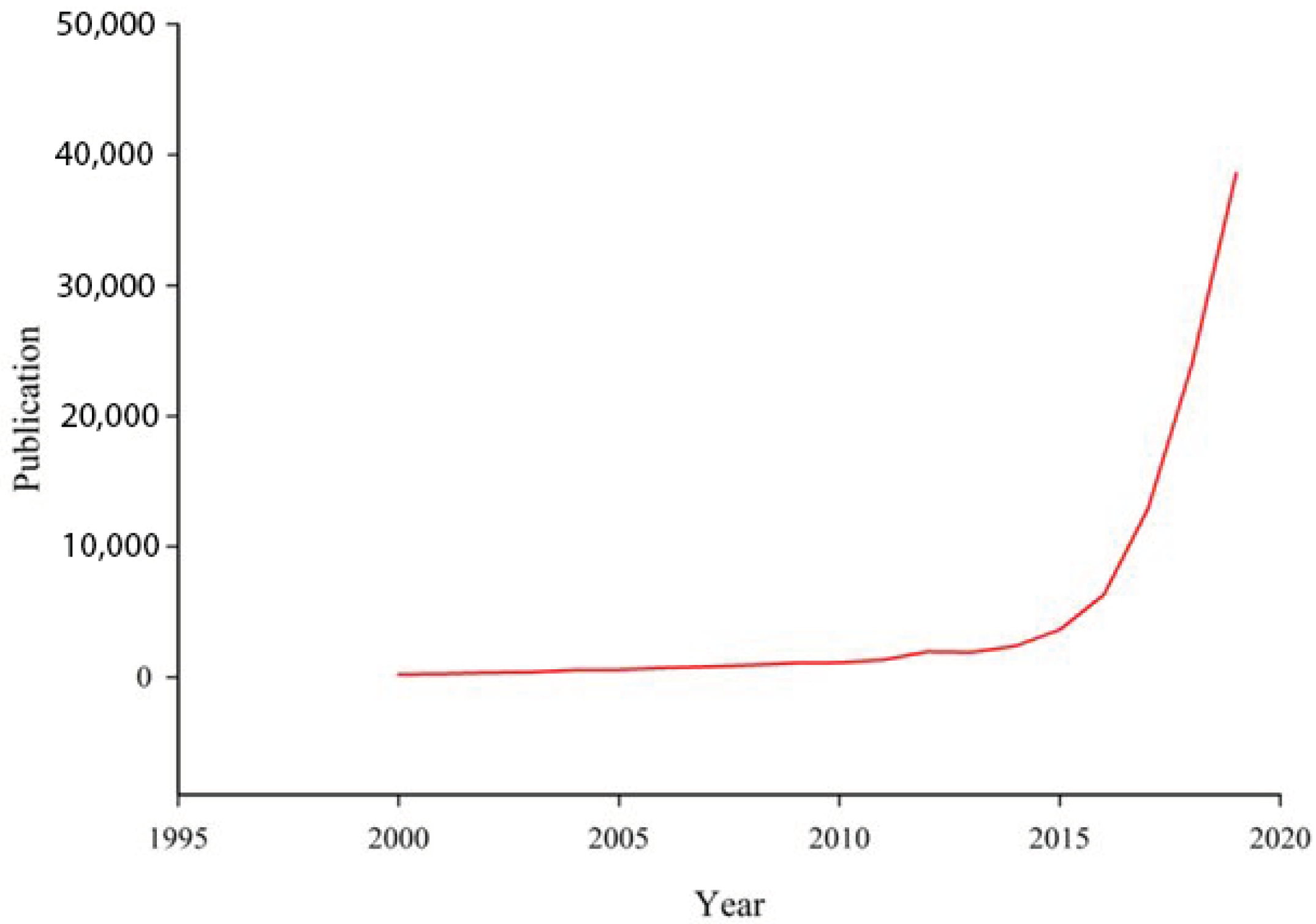
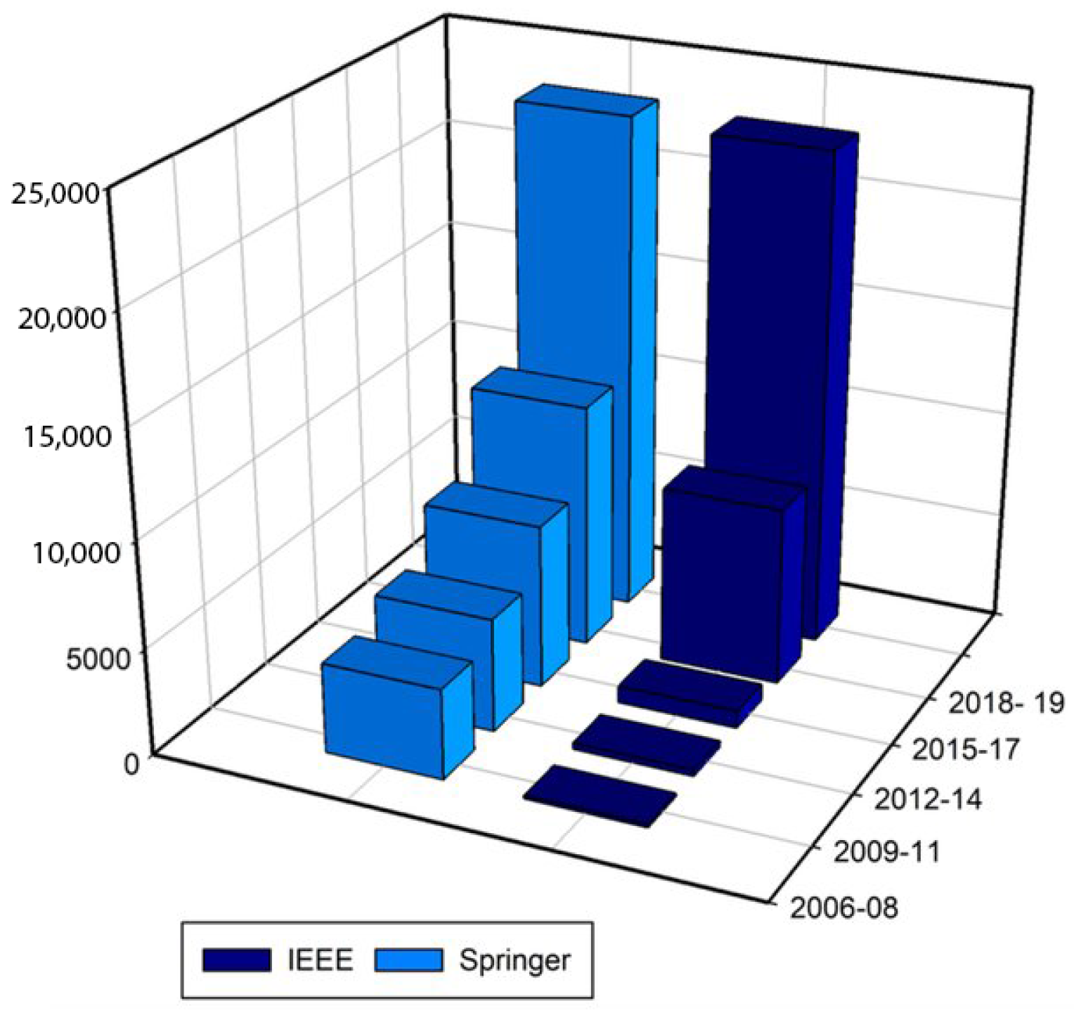
The current interest in these systems is driven by the scientific community and does not appear to have experienced successful adoption among medical professionals. The number of papers applying deep learning to medical tasks has seen a drastic increase in recent years, as can be seen in Figure 1, for the data obtained from Google Scholar using the keyword “Deep learning in the medical field”. As analyzed by [5], the numbers of deep learning publications found in the Springer database and the IEEE digital library for the period 2006–2019 are shown in Figure 2.
Despite the many contributions brought to the field, these approaches seem to be experiencing a roadblock due to being used in the field. This can be caused by a multitude of factors, but the main ones are the inherent lack of explainability of deep learning models [6] which affects their accountability and makes these systems hard to trust for clinical use. This is still a very active subject that is under constant research by the broader deep learning research community, so while there are currently only limited tools to understand the decision-making processes of neural network models, constant progress is being made in this direction. The issue of trust and accountability will hopefully be addressed at some point in the future. Another factor that might slow down the deployment of deep learning systems is the great complexity of the two fields. Both deep learning and medical research are very dynamic domains which are among the most active research fields at the moment. The immense volume of contributions in the field leads to constantly changing states of the art and best practices; while these help push the two fields independently, interdisciplinary alignment becomes extremely difficult as researchers focused on both of them face the difficult challenge of keeping their knowledge up to date.
In this paper, we will approach the subject from the perspective of the computer scientist. In Section 2, after introducing the concepts of machine learning and explaining the difference between supervised, unsupervised, and self-supervised learning, we will present a short description of artificial neural networks and the most relevant types of neural network structures that are actively used. In Section 3, we will review the field of self-supervised learning applied to computer vision. We will emphasizing the importance of these methods for current and future research directions. We will describing the classes of self-supervision algorithms, their benefits, and limitations. In Section 4, we will review how deep learning has been applied to the field of medical imaging, and we will also present how self-supervised learning methods in particular have been adapted and discuss the elevated impact that work on these methods can have on medical image analysis tasks. In addition to presenting the relevant concepts from this field, we will also present the ecosystem of datasets, tools, and communities which should prove useful to prospective researchers in deep learning medical image analysis. We hope that this will help improve alignment between the two fields and reduce the aforementioned interdisciplinary friction caused by the dynamic natures of these subjects. Section 5 will present an overview of the ecosystem of working in this field, describing the hardware, tools, and datasets used in this research.
2. Overview of Deep Learning Methods
In this section, we will attempt to provide a short introduction to the relevant types of neural networks and architectures currently used in the deep learning research community. While traditional machine learning algorithms can be and have been successfully used in the medical field, we will keep our discussion focused on deep learning methods according to the purpose of this work.
2.1. Machine Learning
Machine learning is a sub-field of artificial Intelligence, which studies ways to build intelligent programs which do not require explicit programming and can learn dynamically from the data it is given. Generally speaking, machine learning algorithms would be classified as either being supervised or unsupervised. Supervised learning trains a model by utilizing both the input data as well as a target label. The general purpose of supervised learning is to teach the algorithm to output the associated label for a given sample. While the labels themselves can take various forms from categorical and numerical values to more complex structures such as segmentation maps or augmented images, supervised learning is often thought of as learning an input–output function or relation by training on examples of such pairs.
Unsupervised learning refers to algorithms that utilize data without using labels and are generally used to analyze a set of data to discover patterns in it. The classic example of an unsupervised algorithm is clustering, it uses the data to identify latent structures in the data. One important nuance related to unsupervised learning is its relation to self-supervised learning as the two classifications have often been confused. Self-supervision, just like unsupervised models, only utilizes the input data, but they do so by automatically constructing labels directly from the input. For example, using the input sample as the label for the model. Recently, the understanding of the concept utilized by researchers seems to move towards classifying self-supervision as a subset of supervised learning since the fundamental model training mechanism is the same regardless of how the label is constructed. Using self-supervision together with supervised learning has the benefit of allowing the use of unlabeled data which is easier to obtain, and needed less labeled samples to train a model. Prominent deep learning research figure Yann LeCun describes it as:
I now call it “self-supervised learning” because “unsupervised” is both a loaded and confusing term. In self-supervised learning, the system learns to predict part of its input from other parts of its input. In other words, a portion of the input is used as a supervisory signal to a predictor fed with the remaining portion of the input. Self-supervised learning uses way more supervisory signals than supervised learning, and enormously more than reinforcement learning. That is why calling it “unsupervised” is misleading.
2.2. Artificial Neural Networks
Artificial neural networks (ANN) are a type of machine learning algorithm that try to imitate the biological structure of how neurons function. The majority of ANN models are trained in a supervised or self-supervised manner, while the specific exceptions of unsupervised learning such as self-organizing maps [7] or growing neural gas networks [8] do exist. In the literature, some self-supervised models are sometimes referred to as unsupervised, although our current understanding of the concepts would consider that to be incorrect.
A neural network is composed of neurons whilst a neuron is composed of its parameters in the form of weights and biases together with an activation function, as can be seen in Figure 3. The neuron receives one or more inputs and calculates the output as , where is the activation function, usually a non-linear function such as the sigmoid or tanh functions, w is the set of weights, b is the set of biases that the neuron learns, and x is the input data for the neuron. The output of a neuron is also referred to as the activation.
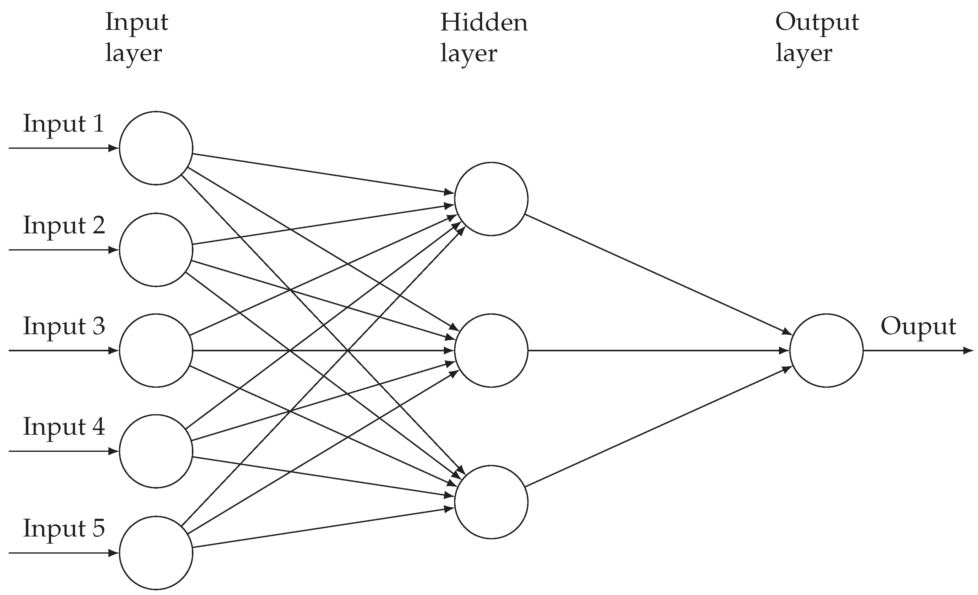
Multiple neurons together are referred to as a layer. Stacking multiple neural layers forms the traditional multi-layered perceptron (MLP) where the output of the previous layer of neurons constitutes the input for the next layer, as can be seen in Figure 4.
These models are trained by means of gradient descent coupled with backpropagation, For this, the loss for a given sample and its label is calculated by comparing the output of the model with the expected label. The loss function indicates the performance of the network and using gradient descent, the weights of the model are optimized to reduce its value. The training process iterates through a dataset in a series of batches of samples, updating the parameters at each step. Repeating this process makes the model learn to predict the correct label for a given sample since it has been trained to generate an output similar to the expected target.
Deep neural networks, networks that stack many layers have historically been hard to train. The first successful approach to training such a model was achieved by pretraining the model layer by layer or by carefully engineering the model architecture such that it does not lead to exploding or vanishing gradients [9].
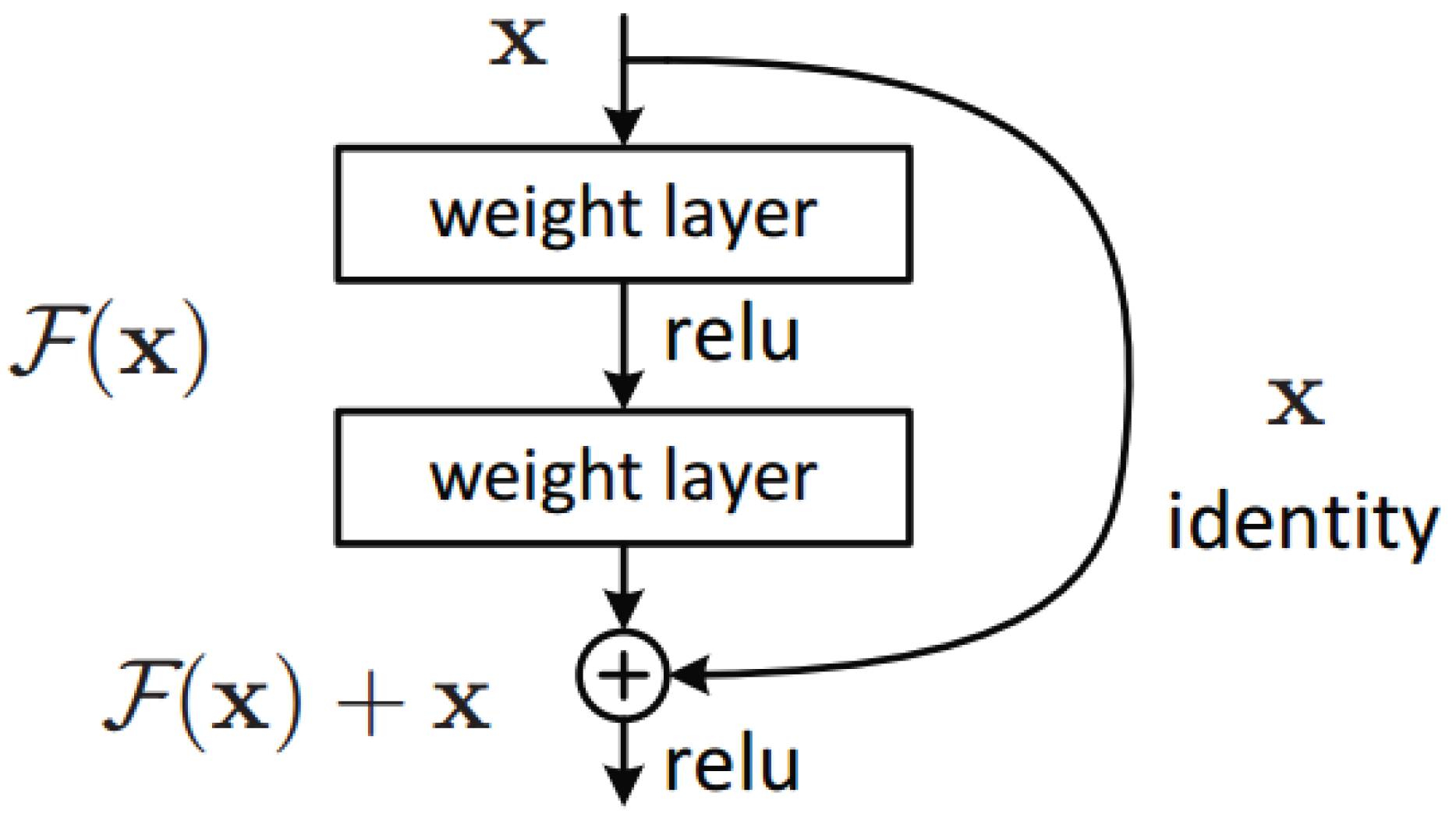
Training deeper models has been enabled by the appearance of residual neural networks [10]. Through the use of residual connections, neural network modules did not have to learn to “carry” the input along the forward pass since the input would be carried by the skip connection. As a consequence, this allows gradient back-propagation on much deeper networks without vanishing, since it can flow through the residual connection, as shown in Figure 5.
The main classes of neural network architectures which have appeared over the years are recurrent neural networks (RNNs), convolutional neural networks (CNNs), and the recent attention/transformer-based models. They each have different characteristics which lead them to specific use-cases, although researchers have adapted them to be used in various unexpected tasks. For example, even if CNNs were developed to be used on image datasets, they have also been successfully used for natural language processing (NLP) tasks [11].
2.3. Recurrent Neural Networks
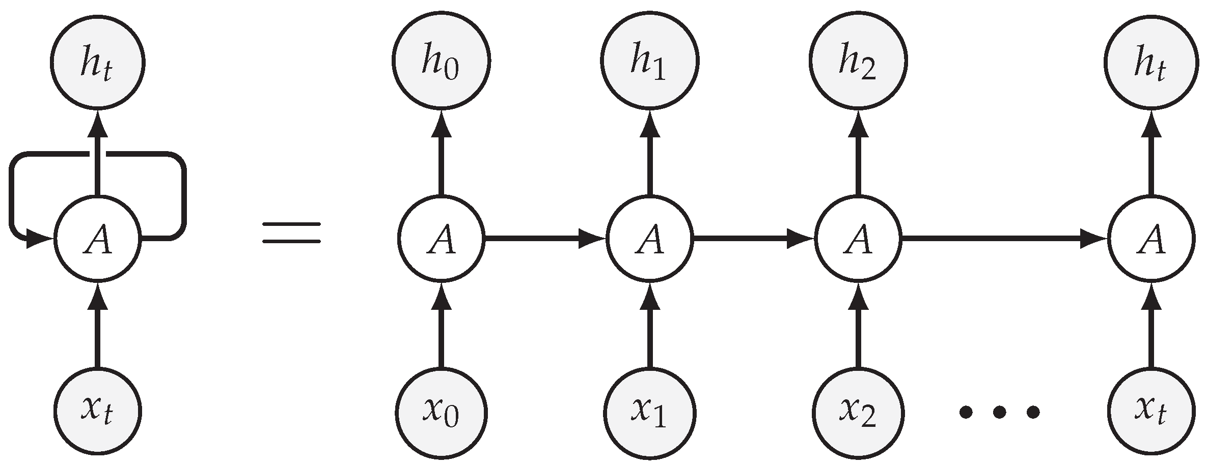
Recurrent neural networks were developed to capture temporal relations in the data. RNNs use their internal state (memory) to process the variable-length sequences of inputs such as time series data or sequences of words in a sentence. They do this by adding recurrent connections to neuron cells, using the same cell to process incoming sequential data, an example unrolling from the calculation made by an RNN cell processing a sequence of of inputs (), as shown in Figure 6. Their main purpose was to process NLP and time-series data.
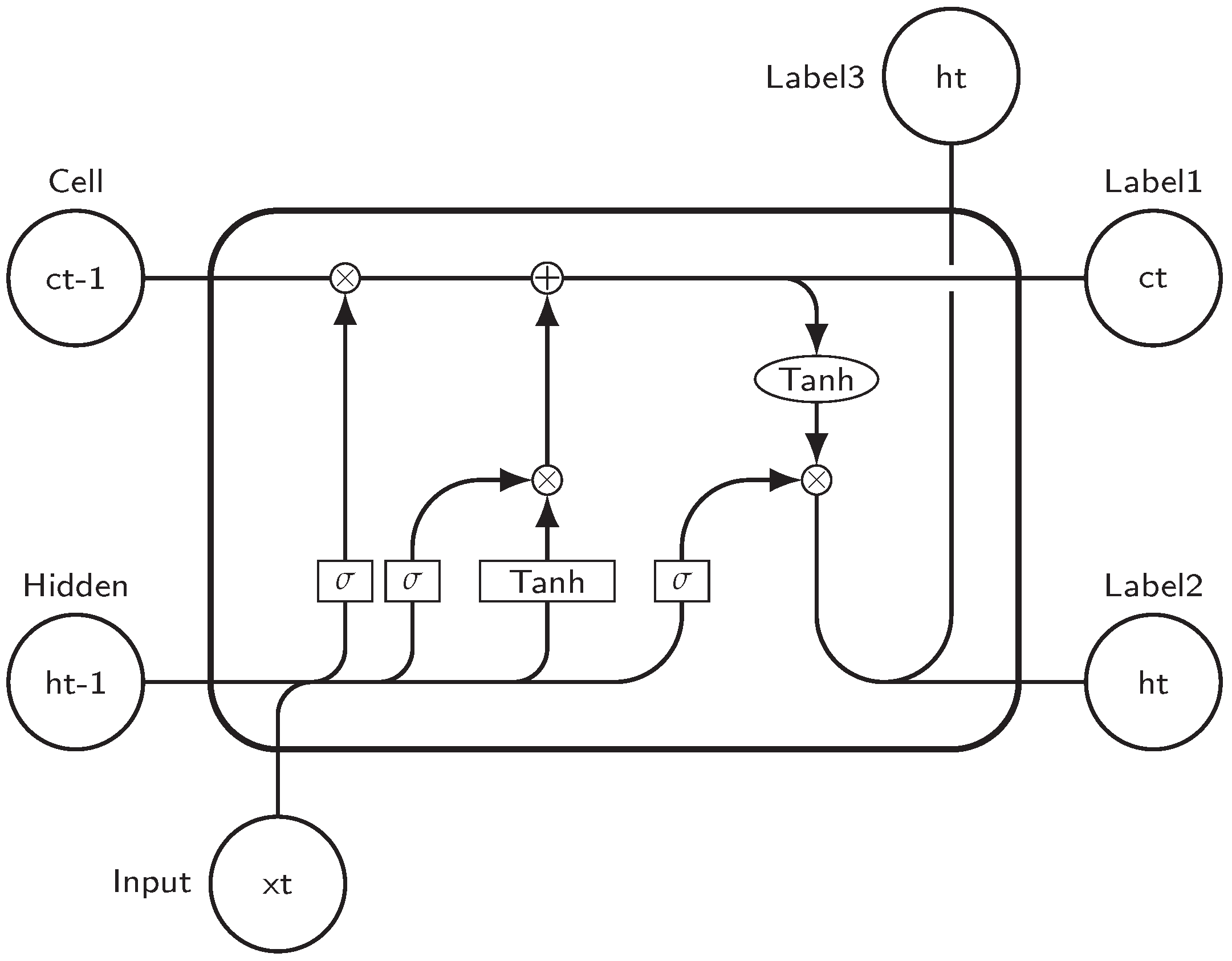
The most popular approach was introduced by [12] known as long short-term memory (LSTM). While effective at mitigating the gradient vanishing problem, its complex structure (Figure 7) and the fact that it requires iterative calculations made it hard to use in scaled-up models which are trained on large datasets.
2.4. Convolutional Neural Networks
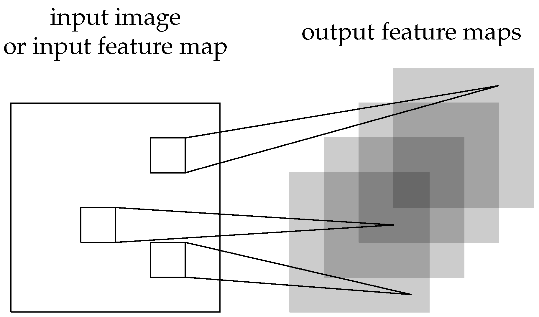
Convolutional networks have been developed to model visual data. Fully connected neural networks have to learn the potential appearance of a pattern in the data for each possible position in an image. The convolutional mechanism uses the same weights to analyze an entire feature map, making the algorithm detect features in data wherever they are present in the image (Figure 8). Because of this translation invariance, convolutional neural networks do not require as many parameters to learn data, and as such, are less prone to overfitting. Another big advantage of convolutional networks over fully connected ones is the fact that the size of the input data does not matter anymore, as they can use the same number of weights for different images and the model will still be able to detect the relevant features.
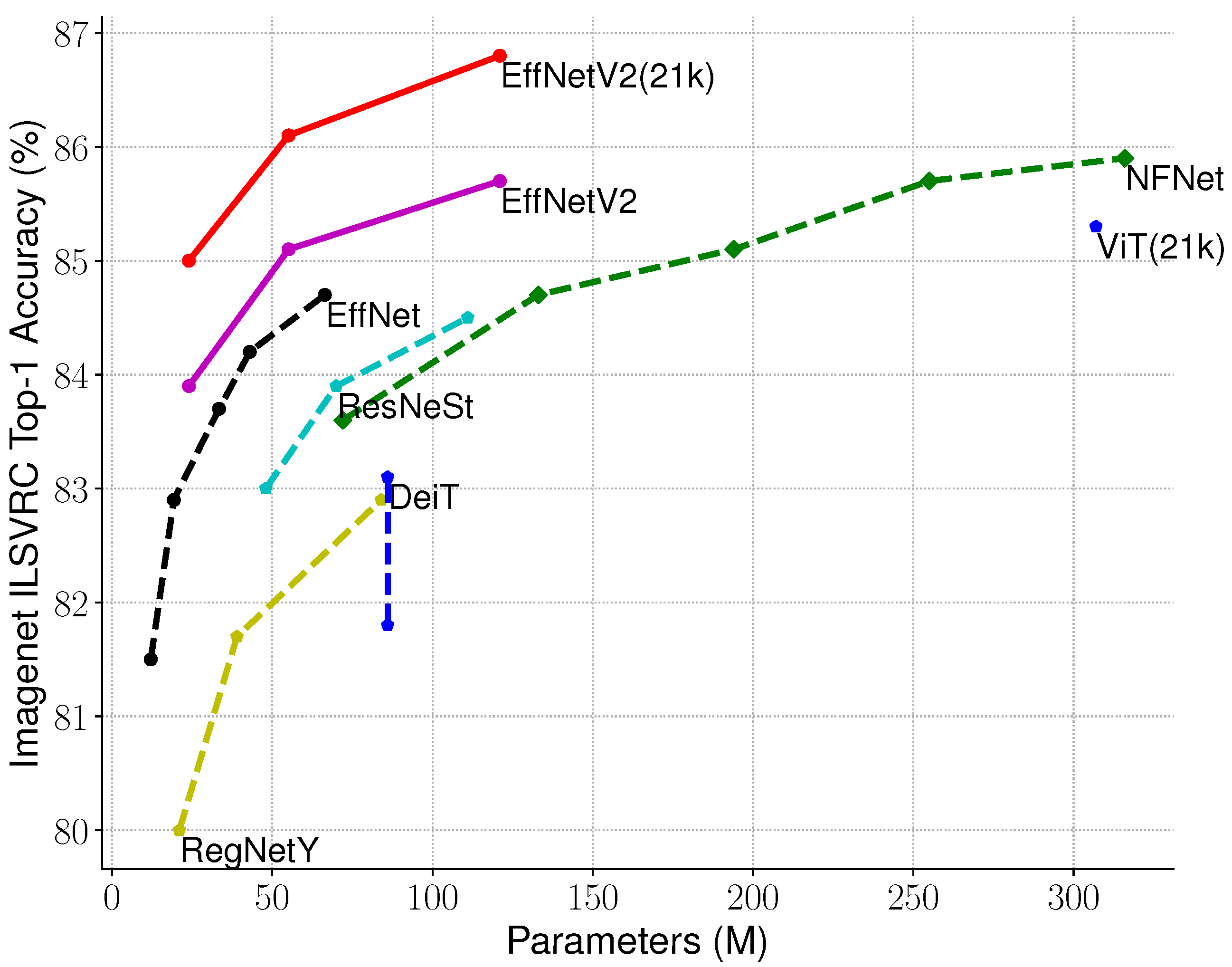
Due to the shared-weights architecture, CNNs can extract a lot more features with the same number of weights as a fully connected network. This, combined with residual connections, has enabled CNNs to be scaled up without suffering from gradient vanishing problems or overfitting. There are successful implementations that use tens of millions of parameters without overfitting (Figure 9).
CNNs have been a primary focus of deep learning researchers for multiple years now; as such, there have been many contributions that improve their performance or adapt them to various tasks. Models have tended to become deeper while utilizing smaller convolutional kernels. This trade-off has enabled to maintain the same number of parameters while allowing the model to capture more complex non-linear relations in the data. The smaller memory footprint and lower computing costs have also enabled the usage of CNNs on mobile devices. There are typically three types of CNNs used:
- 1.
- Classification models use convolutional layers to extract higher-level features, after which a linear layer is used to classify a given sample using these higher-level features into categorical labels;
- 2.
- Segmentation models are generally fully convolutional networks, which do not use any fully connected layers. The final layer of the model outputs a pixel label for each input pixel;
- 3.
- Generative models are similar to segmentation models in the sense that they generally output a value for each input pixel. The difference is that they do not output a label for the pixel but a value that is from the input domain space. These models are used to either generate novel data that resemble real-world images or to augment a given input sample, e.g., to by improving the clarity of details ([14]) or by enlarging regions of interest in the input image.
CNN architectures have been used to great success for both the natural world and medical imaging but have also seen use in NLP tasks due to their great parameter efficiency.
2.5. Attention-Based Models
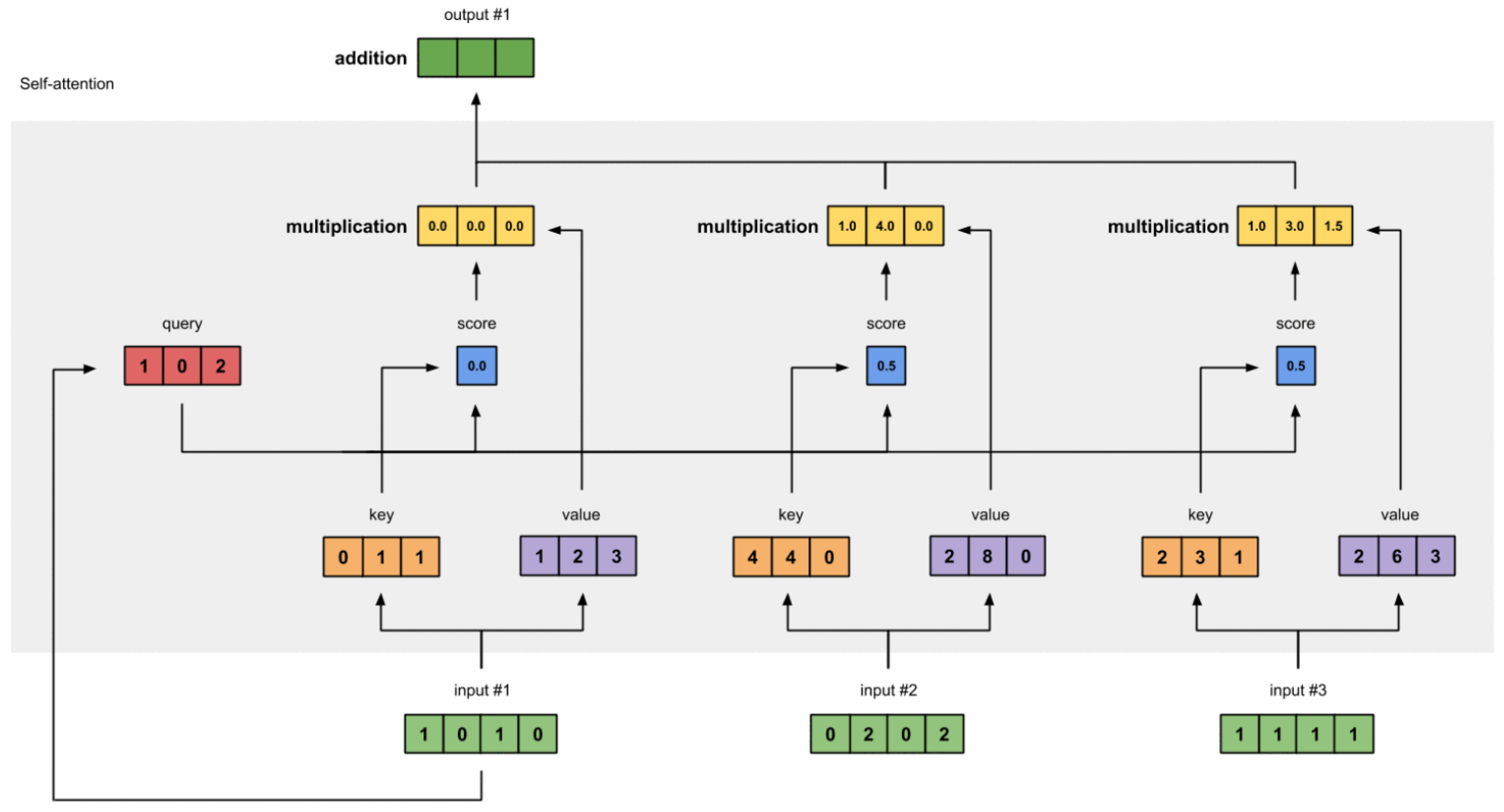
While convolutional neural networks are still the main architecture used for imaging tasks, attention-based models have become the method of choice in the NLP field. Initially introduced in their current form with the transformer model [15], transformers have some important characteristics which have enabled their success. Transformer models utilize an attention mechanism that essentially makes decisions for each input by dynamically looking at all the other inputs to determine the context. The self-attention mechanism has great applicability in sequenced data due to the fact that it is able to capture the context while analyzing each part of the sequence, as shown in Figure 10.
Fully connected layers or convolutional layers will always combine the input values in the same way, aggregating the signals similarly even when the input differs. However, by using self-attention, the way input signals are aggregated is determined dynamically when forward propagating by looking at all the input sequences.
This increase in context understanding comes with a high increase in computing requirements, which becomes clear when analyzing how attention is calculated: . The Q, K, V, vectors (query, key, value in Figure 10, respectively) are obtained by passing the input thought separate linear layers, usually noted as . The term represents the size of the vectors, which is used to scale the dot product such that the resulting score ensures that the properties of Q and K have a mean of 0 and a variance of 1. The use of the scaled dot-product makes the computation intractable for a large number of keys and queries. This issue is being actively researched and several proposals of how to approximate the attention mechanism in an efficient manner have been proposed, such as [16,17].
Attention-based models have seen great success when used in language models. This is performed by feeding a sequence to the model and asking it to output the most likely value to follow in the sequence. By doing this, the model can be trained in a self-supervised manner since labeled data are not required. For NLP tasks, this has enabled the creation of gigantic models since they are able to utilize any natural language text available, such as Wikipedia data, books, news, etc., without having to manually craft labels for these vast volumes of samples. One such recent example is OpenAI’s GPT-3 model [18], which with careful engineering, was able to successfully fit a 175 billion parameter model.
A more interesting recent development in the last two years was the discovery that attention models can be successfully applied to non-sequence data such as images. They have been successfully used for image classification and segmentation as well as object detection, with these models becoming the new state of the art for not only NLP but also computer vision [19,20,21,22]. As transformers have almost completely replaced LSTM for NLP, it would appear that attention mechanisms are going to replace CNNs for computer vision tasks as well. The current limitation is the fact that images are composited of many pixels and this high number of inputs to the network makes traditional attention approaches intractable from both a computing perspective as well as from a memory requirement perspective; however, many new contributions have proposed solutions to these issues.
3. Self-Supervised Learning for Computer Vision
3.1. Motivation
Humanity as a whole is increasingly collecting more data and types of data into ever-growing digital archives. These include anything from images, videos, music, and books to in-app user behavior, biometrics, environmental data, and more. This process has been constantly accelerating as the costs of computing and storage hardware have enabled companies and governments to feasibly gather all these data and extract their economic value.
In parallel with the aforementioned big data push, CNNs have been enabled by innovations in both algorithms and GPU hardware. These two technologies have worked together to produce drastic improvements in many applications, from recommender systems, fraud detection, and malware detection to chatbots, creative, textual and visual tools, design, and more.
While these developments have taken place fairly recently, achieved by using DL architectures and methods which can better leverage more computing power (e.g., transformers [15,20]) and larger datasets, naively training a model to perform a task in a supervised manner has a fundamental problem limiting further performance improvements. While computing and storage can and is scalable with technological improvements and economic capital, quality data labeling is limited by human capital. This issue was not a problem at the beginning since the amount of data needed to be labeled was manageable and increased dataset sizes could be matched by adding more human labelers.
As discussed earlier, the rate of data collection seems to be constantly accelerating and the types of data collected becoming more specific, requiring specialists to correctly label them (e.g., medical, biometric, driving). This appears to be a limiting factor since, arguably, human labeling cannot be scaled to the same degree as data collection. In order to push forward the state of the art in deep learning applications, we will have to develop methods that enable models to extract useful information from data without supervision.
It is important to note that, extrapolating current technological improvements and data gathering trends into the future, the percentage of unlabeled compared to labeled data we have access to will only continue to increase. It is arguably the case that the importance of developing and improving unsupervised and self-supervised methods will be the main driving factor for improvement in the field of machine learning going forward.
3.2. General Computer Vision Methods
In this section, we will present an overview of the types of self-supervised techniques for computer vision that exist and successful examples of them in the literature. We will also present what attempts have been made to apply SSL to medical data.
As a general description, SSL is at the intersection between supervised learning and unsupervised learning. Particularly, SSL does not use labeled data or learn from then, but it does train using “pretext” tasks in a supervised manner. Pretext tasks are tasks that generate their own labels from the data, and these labels are referred to as pseudo-labels.
Self-supervised learning is primarily focused on the designing, training process, and pretext tasks which would force the model to learn general features from the data. Despite several types of such methods existing, the main fundamental issue they need to address is model collapse to trivial constant solutions. This problem arises in self-supervision since the labels that are used are generated by our algorithm, which does not necessarily reflect a meaningful classification in the sample domain.
The taxonomy of how different methods are classified is not completely settled in the literature, which has led to some works often having contradicting descriptions. Despite this confusion, we will try to separate and define the different types of self-supervised methods by what would be the most useful differentiation, which we consider to be the way each technique constructs pseudo-labels from the input data. We will not be describing every individual method in the literature but we will be exemplifying the underlying mechanism that makes the same class of methods work.
3.2.1. Predictive Methods
As among the first self-supervised methods to be successfully applied to computer vision, predictive methods work by constructing a classification or regression pretext task.
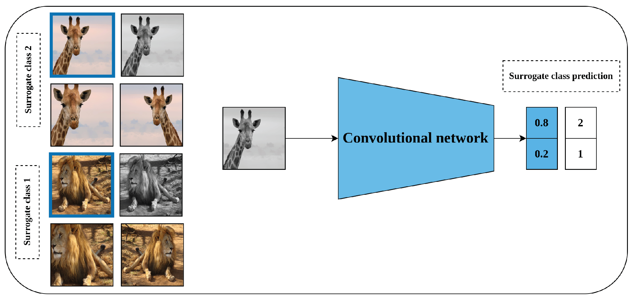
CNN Exemplar [23] is one of the earlier proposed methods of this type. This method works by choosing a small number of samples from the dataset and generating multiple transformations of these samples. Each sample from this augmented dataset will have the index of the original sample it was constructed from as a label, as can be seen in Figure 11. Afterward, a model is trained on this artificially constructed image classification problem.
The most widespread type of predictive methods are different types of geometric transformation predictions.
In a practical sense, geometric transformation predictive methods usually alter the input sample in some way such as rotations, shuffling, contrast, etc. and the task of the model is to predict what transformation has occurred. The most widespread method is known as Jigsaw [24].
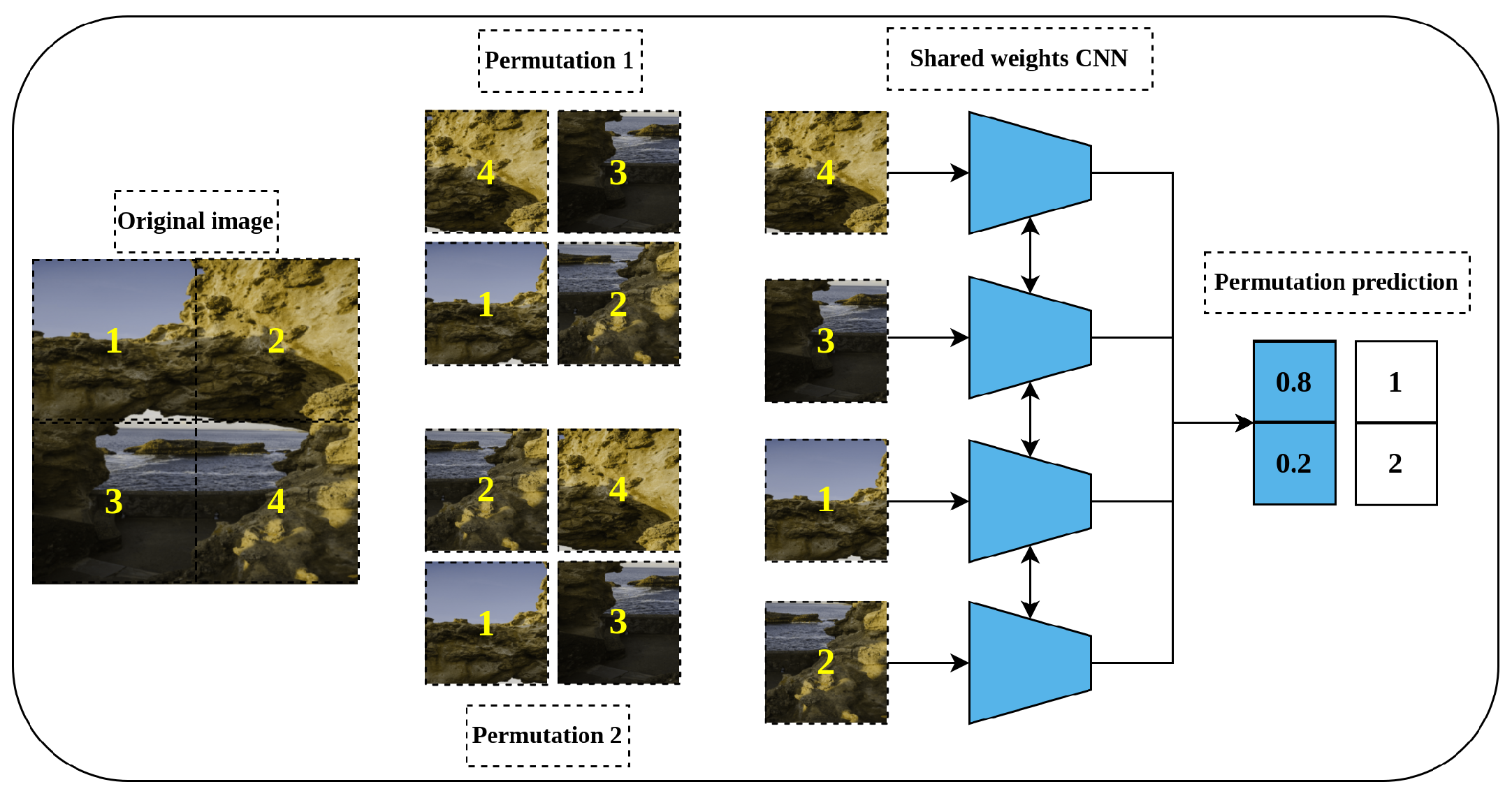
Jigsaw work, by dividing the input images into patches, usually a 3-by-3 grid, generates a permutation of these patches to generate a scrambled image. The model’s task is to predict which permutation was applied to the original image, which is represented as a classification task where the label is the index of the permutation in the collection, as seen in Figure 12. There are several limitations, such as the fact that there are too many possible permutations, requiring a method to select a subset of them to work with, but this introduces a new problem of selecting “good” permutations. A similar method that inspired the jigsaw is predicting the relative position [25], for a given anchor and sample patch from an image, as the model has to predict where the sample patch is positioned relative to the anchor.
Another example of a predictive method is rotation prediction [26], which follows the same logic of predicting which transformation a sample suffered, but in this case, the transformations are different rotation angles.
3.2.2. Generative Methods
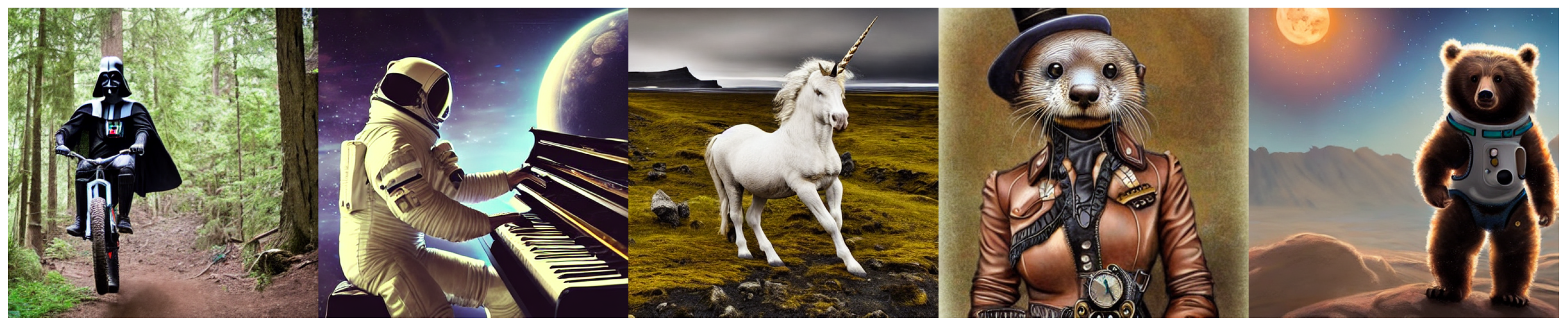
Generative methods are methods that work by asking the model to generate credible artificial data points. There is an increased amount of interest in these methods from the general public due to their applications in AI art generation. One recent work capable of generating images, which has been made easily available, has been Stable Diffusion [27]. This model was extensively trained by Stability AI and pretrained versions have been made available under an open source license. This has led to many extensions and improvements of the implementation and the model is now capable of generating very high-quality images on consumer-grade GPUs, examples of which can be seen in Figure 13.
Autoencoders are among the simplest and most flexible types of generative methods for images which have been widely used in the field of natural language processing (NLP), and they have been put to work in many forms ([28,29,30]). They work by training a model to replicate the input samples in its output neurons. A naive implementation of such a model might lead to model collapse since the model could simply pass the unaltered input all the way through to the output. To combat this, a bottleneck can be applied in the deep model at one of its hidden layers, to reduce the number of neurons to be significantly less than the preceding and following layers, forcing it to learn meaningful features or at the very least, compress the input domain in a denser latent space. They can also be trained to generate new data points from random noise with variational autoencoders (VAEs), which instead of encoding a compressed embedding, the encoding is represented as a mean and the covariance matrices of a Gaussian process. By doing this, the encoding can be sampled for data which can be decoded to obtain novel generated content.
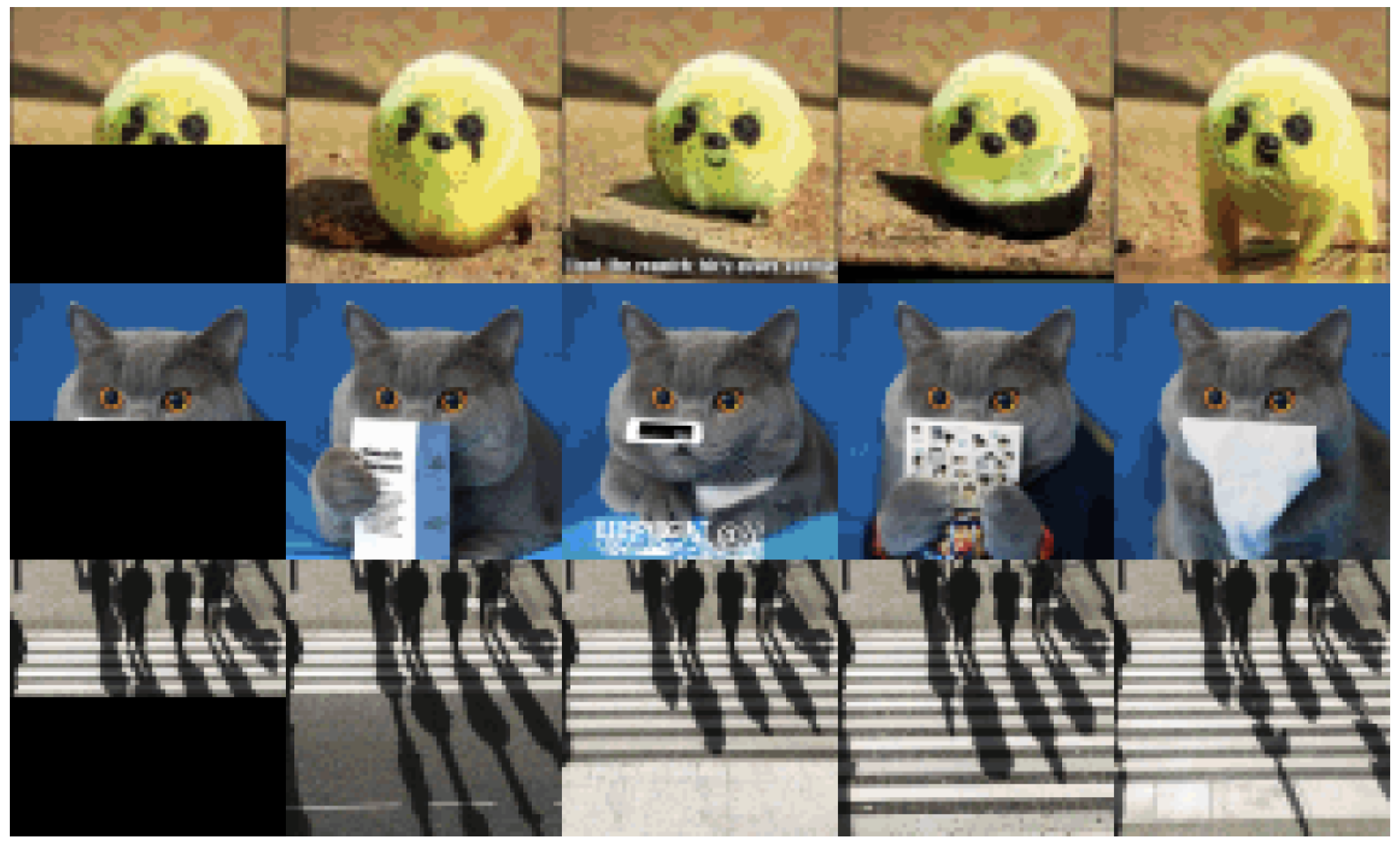
Another way to avoid trivial constant solutions is to also transform the input. Tasks such as super-resolution, low-light enhancement, or artifact correction could be used for this. Specifically, for super-resolution, the input image is down-scaled to reduce its resolution, asking the model to reproduce the original quality image, similarly for low-light enhancement and artifact correction, the brightness of the image is reduced, or randomly generated artifacts are introduced, training the model to return the input to its original state. Another powerful example of such a task is pixel masking, which can be done by randomly deleting or masking parts of an image, the model having the original image as its target [22].
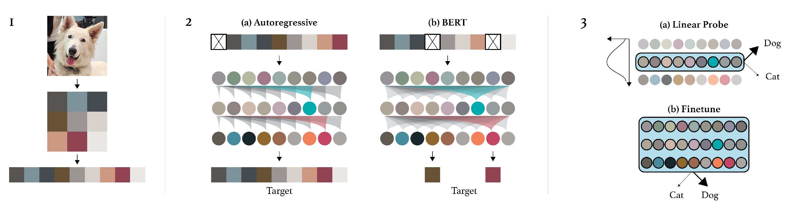
Inspired by NLP, the method Autoregressive Next Pixel Generation [22] was adapted from language models. This works by sequentially asking the model to predict the next pixel or patch of pixels in a sequence, as can be seen in Figure 14. A 2D image would first be flattened and then formed into a sequence of patches or individual pixels. The current sequence of pixels is passed through the model and the target of the task is to predict the next pixel or patch in the sequence. Since the next pixel in the original image is known, it will be used as the pseudo-label. Both pixel masking and autoregressive generation can be seen in Figure 15.
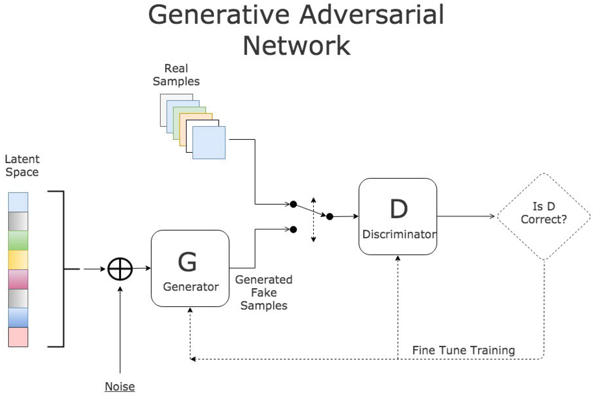
Lastly, potentially the most widely adopted generative self-supervised method, is that of Generative Adversarial Networks (GANs) [31]. These models are composed of a generator, which takes random noise (or trained latent scrambled with random noise) and produce an artificial sample and a discriminator which has to detect whether a given sample is real or generated; the generic GAN architecture can be seen in Figure 16. Despite being the most structurally complex of the generative methods, GANs have seen much more use from both the academic and general public.
3.2.3. Contrastive Methods
Contrastive methods are a more recent development, they are constructed using joint embedding architectures. Training is performed by constructing two different augmentations of images together with other samples and passing them separately through Siamese networks. The output two embeddings are then used to calculate a contrastive loss, which penalizes the distance output embeddings of transformations from the same original data point, called positive sample pairs, while pushing away output embeddings that originated from different samples, named negative sample pairs.
The main issue facing contrastive methods is the need for quality-contrastive negative pairs, since negative pairs are made to lead to distant embeddings, an issue that arises with the fact that oftentimes, images, while different, are very similar. Especially since labels are not used, the method will similarly distance semantically identical images to pairs of images that are completely different. For example, two pictures of the same breed of dog will have the same contrastive loss as one picture of a dog and one of an airplane. To counteract this, contrastive methods usually have to use very large batch sizes to minimize the impact of these “noisy” contrastive pairs or additional creative ways of identifying quality negative samples need to be used.
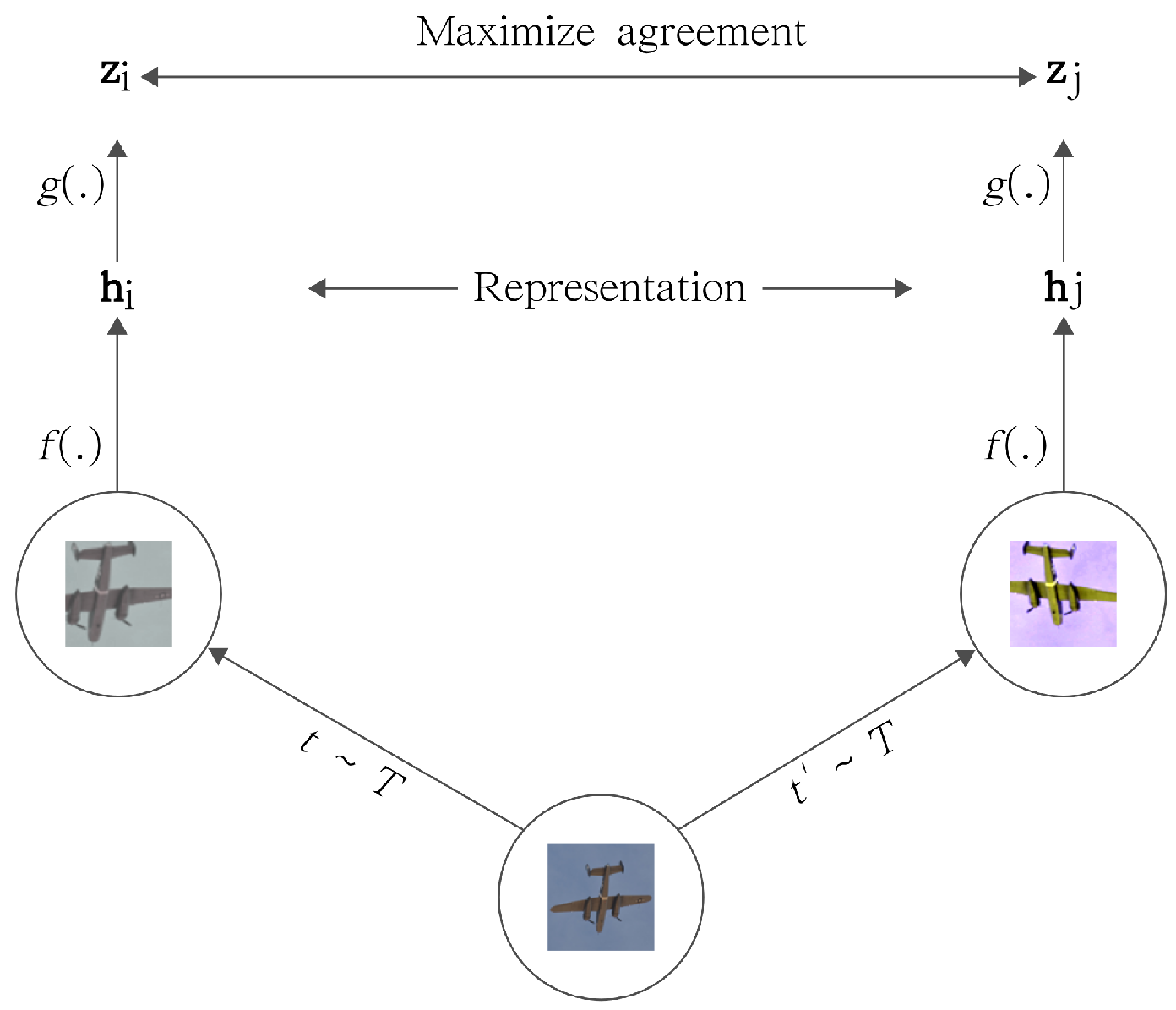
While different proposed methods vary greatly in the exact formulation of the loss used and different tricks of sampling pairs, they will mostly follow a similar structure as SimCLR [32], as can be seen in Figure 17. The loss used is usually the InfoNCE [33] where NCE stands for noise-contrastive estimation. The loss is essentially the multi-class cross-entropy between the matrix product of the two augmented batches of samples () and the identity matrix, where a and b are different transformations applied to the input. The batch is of shape (batch size x output embedding size). The diagonal of the matrix shows the positive pairs while the rest of the matrix shows the scores for the negative samples.
3.2.4. Clustering Methods
While contrastive methods effectively treat each sample having a distinct label, clustering methods first group samples into clusters before calculating the contrastive losses of positive and negative pairs. These methods decrease the need for large batch sizes to address the negative sample issue, however, a similarity metric between samples will have to be defined and clusters have to be formed before the model can be trained.
These methods tend to be hard to scale due to the additional overhead required by clustering and while they do reduce the impact that noisy negative samples have on training, it is essentially still a contrastive method but instead of sample pair comparisons, they will be done at the level of clusters.
3.2.5. Distillation Methods
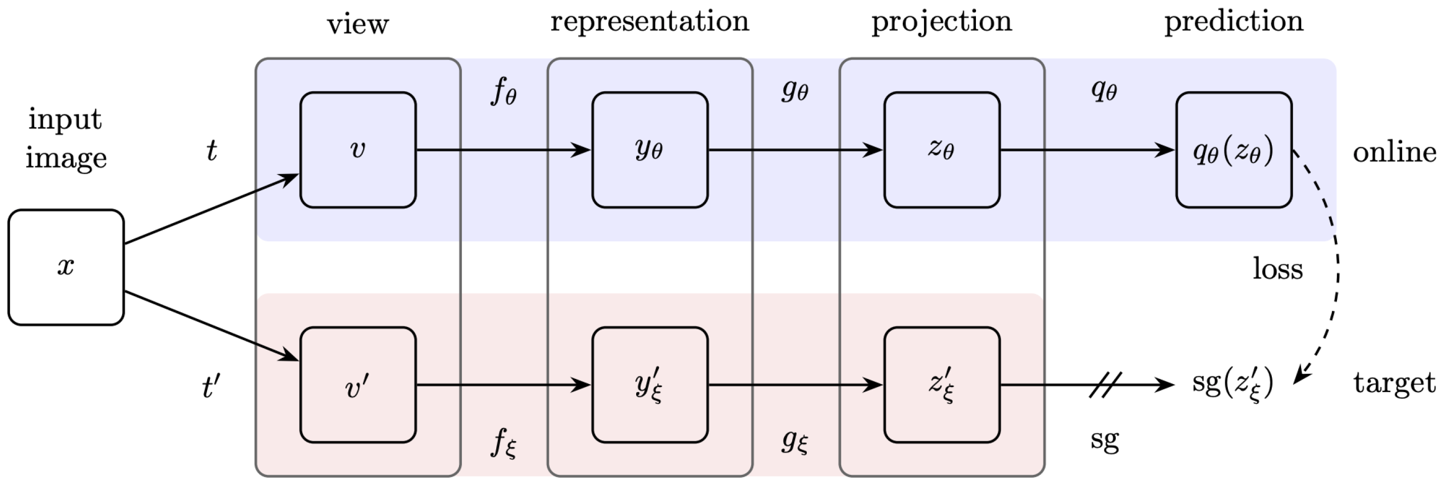
Distillation methods started to appear in 2020 and have since taken over as the main self-supervised learning method of choice. These are heavily based on using dual path networks, each receiving a different view or transformation of the same input batch, similar to contrastive methods. Where distillations differ is that they do not require negative pairs for their loss function. Normally, this would lead to collapse, but BYOL [34], DINO [35], SimSiam [36] and variants work around this by doing architectural tricks borrowed from knowledge distillation.
While some details differ, distillation methods use a student and a teacher model which has the same architecture as the student but its weights are calculated as the running average of the student weights; the teacher also usually does not have gradients propagated to it. For reference, the BYOL architecture in Figure 18 shows that the gradients are not propagated in the teacher, by the symbol meaning “stop-gradient”. The use of different weights in the two models is exemplified by representing the student weights, and which is the exponential moving average of .
The pretext task for these methods is to predict the output embedding (or class distribution in the case of DINO) of the teacher model, as similarity loss is usually minimized. Since negative pairs do not need to be explicitly treated, smaller batch sizes can be used, and the calculations of the losses are simpler. There is no clear understanding in the literature of why distillation models do not suffer from collapse.
3.2.6. Information Maximization Methods
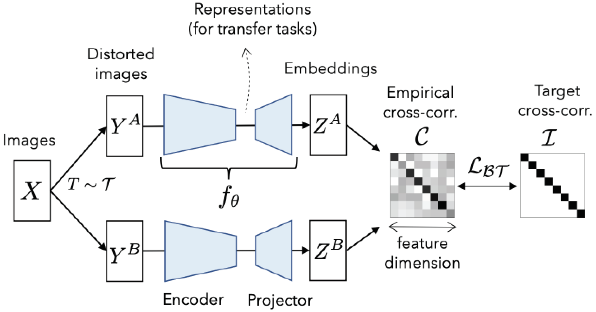
More recently, a new class of SSL methods has appeared in the literature. These methods can be classified as information-maximization methods, among which there are currently only three well-known examples. Two of these originated from Meta AI, Yann LeCun being a co-author in both, namely Barlow’s Twins [37] and VICReg [38].
These methods are currently the state-of-the-art in SSL. They manage to not require a negative contrastive pair of samples but do not have to resort to knowledge distillation tricks to avoid collapse, as they manage this by very simple changes in how they calculate the loss. The simplicity of these methods in addition to their higher training stability, fewer hyper-parameters, and use of a single model renders them very attractive.
Looking at Barlow’s Twins in particular, the architecture of which can be seen in Figure 19, the pretext task is simply that the cross-correlation matrix of the two views needs to be the identity matrix. The loss function, , is:
where is a trade-off variable between the first and second terms of the loss, and is the cross-correlation matrix.
4. Deep Learning Approaches in Medical Imaging
Deep learning has been successfully applied to medical image analysis to help medical professionals in recent years. Machine learning is being used to offer diagnosis suggestions, identifying regions of interest in images, or augmenting data to remove noise and improve results. In this section, we will present an overview of deep learning medical imaging analysis research.
The common issue that various medical image analysis tasks have is the small volume of data available. Compared to natural image datasets such as ImageNet ([39]) which has over one million samples or even smaller benchmarks such as CIFAR-10/100 which has tens of thousands, medical datasets tend to be on the scale of a few hundred samples. Coupled with the fact that medical images such as CT-scans or MRIs have much greater resolutions compared to classic benchmarks and are also 3D, this makes fitting models for such tasks difficult. This high dimensionality of the input alone makes models extremely prone to overfitting and this effect be cannot easily counteracted by acquiring more training data. This problem of small datasets has multiple sources from the legal constraints of data collection and usage to the higher cost of acquisition due to the need for specialized equipment and trained experts to not only obtain the raw data but to also correctly label them. Because of this, methods that manage to increase parameter efficiency and extract more relevant information using fewer parameters seem to perform best.
4.1. Classification
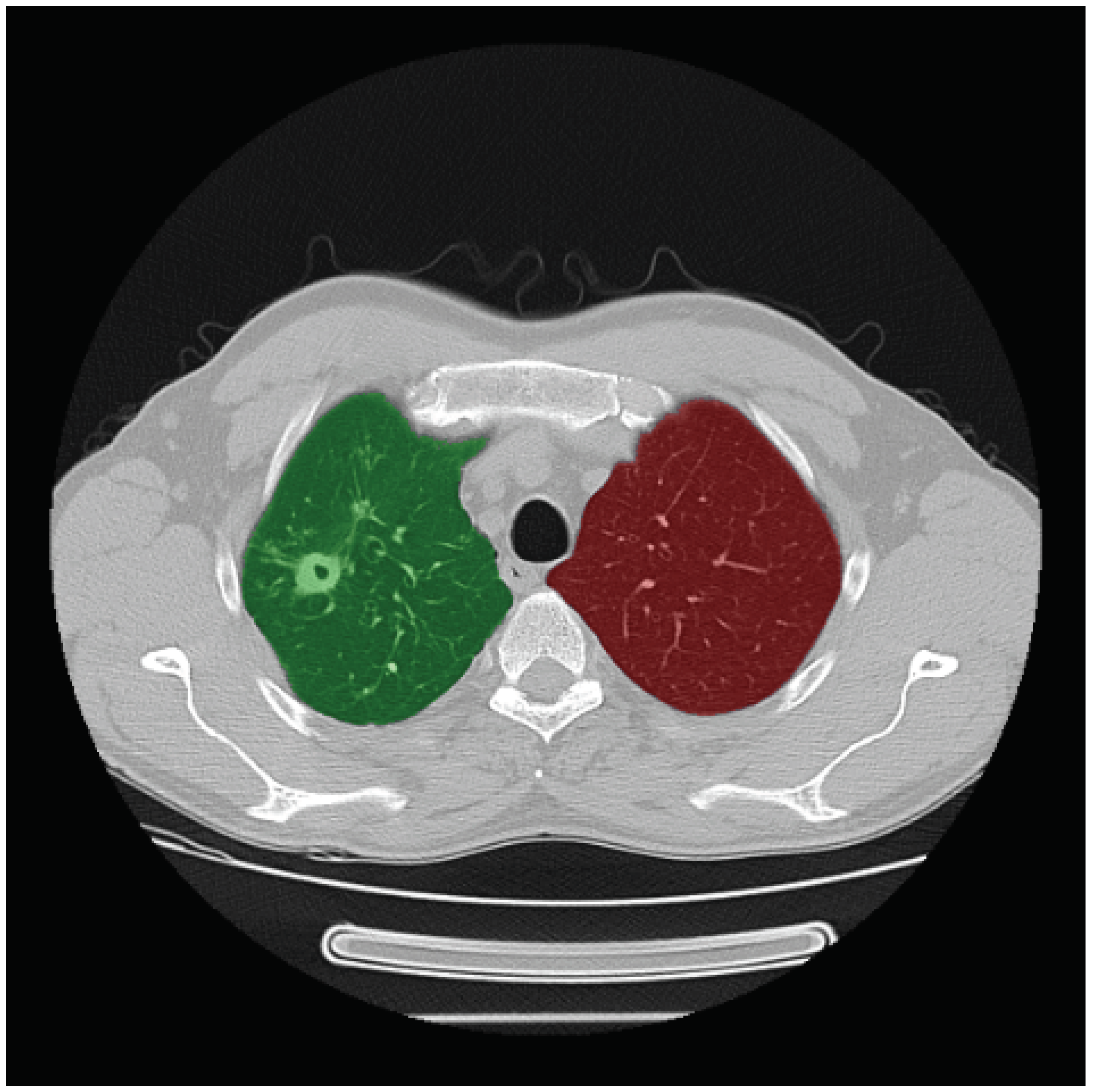
One of the first obvious applications for deep learning in this field is that of classification tasks. Classification is meant to either replace human decision making or at the very least offer a second “opinion” on given data. The classic example of this would be to classify whether, for a given MRI or CT scan, there is a disease present. This type of task can also be modeled to output the level of severity if the disease is present. One such task would be the ImageCLEF Tuberculosis workshop ([40]) (sample slice in Figure 20). Since the diagnosis of a disease is one of the fundamental activities in the field of medicine, deep learning has a wide array of potential applications here since it can theoretically be applied to analyze any diseases doctors have to process today.
As mentioned previously, parameter-efficient models such as Google’s Inception v3 model would seem to perform best in this data-starved environment. They have already been shown to achieve human expert performance in skin-cancer classification ([41]). Another technique used to help with overfitting is pretraining: by initially training our model on other tasks, generally on a big natural images dataset, and then only fine-tuning the model on the smaller medical data, researchers were able to counter overfitting due to the regularization effect that pretraining seems to offer.
As identified by [42], the medical imaging research community has been following the general trends and methodologies developed by the general computer vision field. The initial works in the field utilized deep Boltzmann machines (DBMs) on tasks such as classifying Alzheimer’s disease based on brain magnetic resonance imaging (MRI) ([43]). DBMs use probabilistic variables connected in an undirected model, which are used to learn the representations of the input data by learning to maximize the log-likelihood of the data. This allows for unlabeled pretraining, however, these models are slow for both training and inference, limiting their uses.
Currently, the main architecture of choice for working on brain MRI, retinal imaging, and lung computed tomography (CT) is convolutional neural networks. Advancements in both GPU hardware and distributed cloud computing have also enabled new types of architectures to be employed, such as those using 3D convolutional layers which, despite requiring a lot of VRAM, produce greater results on the majority of medical imaging tasks which are themselves usually 3D images ([44,45]).
4.2. Segmentation
The task of segmentation is typically defined as identifying the set of voxels that either make up the contour or the interior of the object(s) of interest. Segmentation tasks in medical tasks have received great attention from the research community; successfully solving this task can help doctors directly by helping identify regions of interest faster in large 3D scans, but can also serve as a preprocessing tool for classification models. Training classification models directly on sections of data that have relevant information can help training converge towards better results; as such, classification datasets are usually pre-processed by extracting only the regions or organs that are relevant to look at using segmentation.
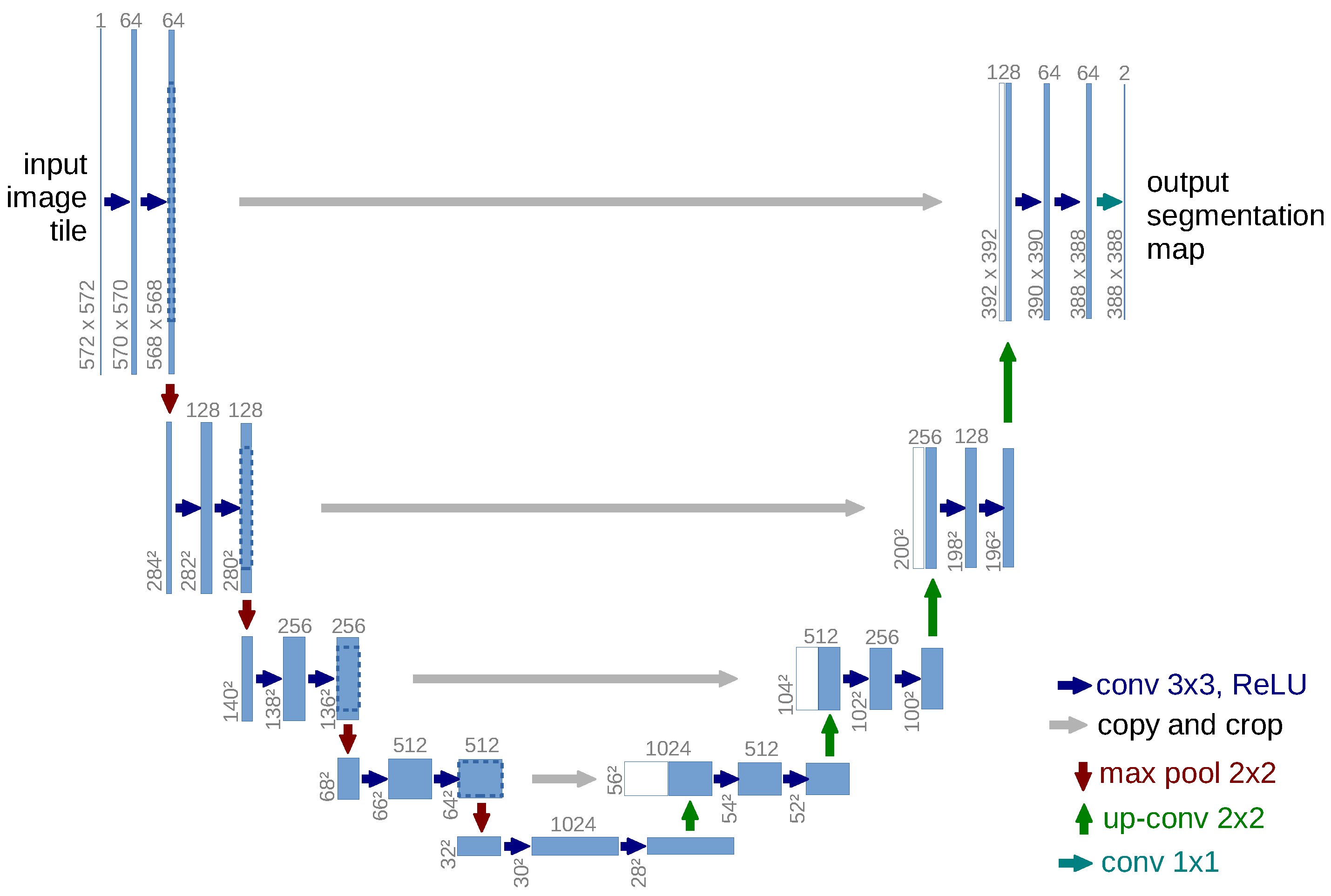
Due to this increased interest in segmentation tasks, this field has seen the development of unique architectures which do not just replicate natural imaging models. The most popular and successful such architecture is the U-Net ([46]). This method leverages the use of the same feature maps used to extract higher-level features to also be used at the final image recreation steps by simply transmitting the signal directly to the decoder layers, as can be seen in Figure 21. Due to the better utilization of their parameters since being reused, U-Nets usually perform better than other segmentation architectures in scenarios where the dataset is small. Multiple approaches have managed to adapt U-Nets to work with 3D data such as [47,48]. Medical imaging has an interesting research advantage of being able to develop unique methodologies for the challenges faced in the field as well as great appropriate contributions from the wider computer vision community; one such example would be DRU-Net ([49]), which expanded the U-Net approach by using convolutional blocks inspired from ResNet ([10]) and DenseNet ([50]). Currently, the state of the art on multiple image segmentation tasks uses U-Net variants or networks which used the principles which make them work. Currently, these models are the U-Net++ ([51]) and, more recently, the MSRF-Net ([52]) architecture.
Another interesting recent development has been the adoption of an attention mechanism in medical image segmentation such as the AttnU-Net ([53]). These models very recently became the new state of the art (SOTA) for many datasets; some simply swapped out components in existing architectures for transformers, and others managed to obtain SOTA with pure transformers, such as Swin-Unet ([54]) and UNETR ([55]). If we are to follow the recent trends in natural image analysis, attention architectures are likely to become new to the state of the art in medical imaging as well. The advantage of capturing long-range feature dependencies will likely be that of a utilized even mode in medical applications, due to the higher resolution and additional volumetric dimension of the images.
4.3. Image Retrieval
A very important task for aiding medical professionals that have seen the applications of deep learning has been content-based image retrieval (CBIR). This is a technique for knowledge discovery in massive databases and offers the possibility to identify similar case histories, understand rare disorders, and ultimately, improve patient care in both speed and quality. The current methodologies are using pretrained CNNs from natural imaging which are fine-tuned on medical datasets ([56,57]).
4.4. Image Enhancement
Image enhancement has been used as a pre-processing technique to help both human experts as well as other AI systems. While initial approaches used rule-based simple transformations to clean up the data or to make important details clearer, this field has seen some interest from the deep learning community. Examples are regular and bone-suppressed X-ray ([58]), generating PET from MRI ([59]), and they have even been used to reconstruct faulty or damaged scans ([59]). Other important applications consist of the classic computer vision task of super-resolution which takes lower resolution inputs and upscales them while keeping image clarity [60]. The same methods can be used for denoising or intensity voxel normalization. Usually, CNN architectures are pretrained and adopted for these tasks although for some of them, specific medical architectures such as U-Net have been used successfully as well.
4.5. Self-Supervised Learning for Medical Imaging
The medical field has also seen research into applying machine learning to perform various tasks:
The usual characteristic of medical datasets sustains the case for researching self-supervised learning specifically for medical image analysis. Firstly, the scale of labeled datasets is little in comparison to what the general computer vision field is working with currently, such as ImageNet21K, Google’s JFT-300M, or Meta’s IG-3.5B-17k datasets. This discrepancy between the fields is expected as the volume of medical imaging is smaller and the number of qualified specialists who can label and compile these kinds of datasets is drastically lower.
Another factor to consider is that medical images tend to be very large and contain fine details; intuitively, it is plausible that a medical image would contain more information in it than a comparable general image. If this is the case, SSL has the potential to learn more from the sample itself.
Finally, medical datasets generally have more overlap between them even if designed for different tasks. For example, a brain MRI dataset of healthy and Alzheimer disease patients will share a lot of the general features and information as a brain MRI dataset of brain cancer patients. If performing classification for the two diseases is desired using only supervised learning, this would require the training of two different models separately on each dataset. Self-supervision brings a great benefit, allowing the pretraining of a single model using both datasets, hopefully learning more general features which should lead to better downstream task performance. This overlap of information between datasets, even if designed for different tasks, can even be expanded to the datasets of scans in different modalities, but which reference the same organ. For example, a brain CT, brain X-ray, brain MRI, and brain PET all capture different properties (structural, compositional, functional) and represent a different modality, but they will all have shared information due to the fact that the underlying organ being scanned is the same. Potentially, even modality information across different organs, e.g., the X-rays of both chest and bones, could be captured by SSL methods, for which it would not be possible to design a supervised task to do the same.
All the SSL methods described in the general computer vision section could be applied to medical images with little to no alterations; however, the field has only recently started applying them in this context. We suspect the limiting factor explaining why these methods have not seen the same degree of adoption for medical images, is the fact that self-supervised learning generally requires a lot more data to train. The luxury of having large amounts of additional unlabeled data in general computer vision contexts is not common for medical images. Another potential reason is the fact that medical images are generally more sensitive to aggressive augmentations since small details are of greater importance. Having fewer data to work with, while also having to limit the scale and number of data augmentations used, probably lead to SSL methods not being an ideal choice to employ.
There are a few specializations of the methods described above which have shown potential.
4.5.1. Predictive Methods
Since they were also the earliest self-supervised methods in general computer vision, predictive methods seem to have been experimented with the most in the medical domain.
The Jigsaw method has inspired several medical versions; in [61], the authors proposed a slice ordering task, the model received two slices, and the model has to predict which one is positioned above the other. Another Jigsaw extension was the 3D Jigsaw [62], which is similar to the original Jigsaw task, just that the patches are now 3D. Still inspired by Jigsaw but, with a more novel approach, Rubik’s Cube [63], is a method of breaking the image into multiple small 3D patches, shuffling and rotating them, and the model has the task of trying to reconstruct the original image, having to predict both which rotations and what ordering the patches are in.
Other works leverage the standardized structure of medical scans by creating the tasks of predicting distances between random patches, slice positions from scans, etc.
Predictive methods are simple, easy to train, and can beat models which are only trained using supervision; however, they do not performing as well as other types of methods.
4.5.2. Generative Methods
Since there is no interest in medical image “art”, generative methods for medical images have mostly focused on color correction, artifact correction, and super-resolution tasks ([64,65,66,67]). Generative methods seem to have been successful in these reconstruction tasks. There are multiple variations in how they construct the loss and the label but the fundamental mechanism remains unchanged from the general computer vision ones.
A more substantial novel contribution origination from the medical field is the use of multiple image modalities for generative models. Since some pathologies require multiple types of scans, some works propose the task of restoring one modality from another [68], or to extract some information from one modality and use it to create pseudo-labels for training on the other modality [69].
4.5.3. Contrastive Methods
SimCLR and MoCo have been applied to medical tasks and achieved good performance. However, not many domain-specific adaptations have been made. An interesting contribution has been to use slice “regions” as positive samples [70] since the medical images of the same organ tend to be very similar structurally between patients. Another interesting idea comes from a SimCLR-inspired framework [71], where they showed that you can construct positive samples using patient metadata, such as treating multiple scans from the same patient as positive samples.
4.5.4. Distillation Methods
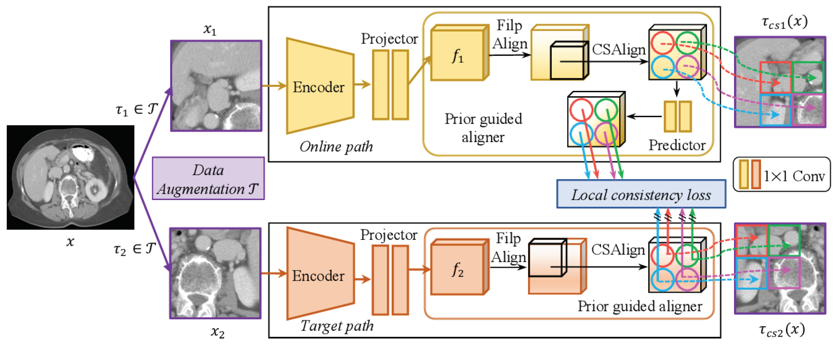
Inspired by BYOL, prior-guided local (PGL) [72] learns spatial and regional consistencies by looking at the differences in the latent space features of two views of the same image. This manages to maintain the high level of detail present in medical images. Their method works by generating the two views from doing random 3D crops and storing the information concerning where the crops took place. They used the location wherein the two views overlap to estimate where the embedding feature volumes would overlap and will only calculate a positive pair of contrastive loss between the overlapping sections. See Figure 22.
Results show this BYOL adaptation reaches state-of-the-art performance on several benchmarks.
4.5.5. Information Maximization Methods
We have not found any reference in the literature to the use of information-maximization methods to date, but judging from how the other SSL methods have performed on medical tasks, we expect them to be able to push the state of the art.
5. Ecosystem
5.1. Hardware
On the hardware side of things, there has been great generation by generation leaps in CUDA computing capabilities: the new Nvidia RTX 3090 GPU features 10,496 CUDA cores compared to the previous generation’s 2080 Ti card’s 4352 CUDA cores. The new card even runs at higher clock speeds with a 1395 MHz base clock and a 1695 MHz boost compared to the 1350 MHz base and 1635 MHz boost of the RTX 2080 Ti. For deep learning in particular, specialized hardware must be included such as the tensor cores for FP16 computing capabilities. Both Google’s TPUs and Nvidias newer cards have included hardware capabilities for new data types developed specifically for deep learning workflows such as brain floating point (bfloat16) or TensorFloat-32 (TF32), which maintain the practical accuracy and numeric stability required by deep learning while reducing the memory requirements to almost half.
One problem that the hardware space faces, and which can be seen to taking place, is the fact that Nvidia currently holds a monopoly on deep learning hardware. Although AMD, and more recently Intel, are also developing GPU, they lack the already adopted CUDA software integration and R&D capital expenditure to produce comparable products. The other players in this space are the Google TPU which they do not sell to customers and are only available through their cloud platform or up-and-coming startups such as Tenstorrent (https://tenstorrent.com), accessed on 10 September 2022, which are very promising but have yet to reach the market.
5.2. Tools
The other driving force behind the popularity of deep learning methods is the wide availability of open source software packages. These libraries provide the efficient GPU implementations of important operations in neural networks. The current dominant frameworks are PyTorch and Tensorflow, and although they are available in multiple programming languages, the dominantly used one remains Python. These big frameworks are aided by a plethora of other packages such as OpenCV, Pillow, Scikit-image for image processing as well as Numpy and Pandas for working with data. Specifically for medical imaging, many packages were developed to visualize, analyze, annotate, and pre-process the various file formats which were obtained from MRIs, X-Rays, and CT scans.
Since there has been such a widespread adoption of frameworks such as PyTorch, this makes the reproducibility and improvement of academic paper results much easier since people can easily share their implementations on source control platforms such as GitHub. One useful website developed specifically for this purpose is https://paperswithcode.com/sota, accessed on 10 September 2022, which tracks the state-of-the-art paper results in various machine learning fields and where their various implementations can be found.
5.3. Datasets, Workshops, and Competitions
While there have been a lot more workshops and competitions on natural imaging tasks, medical image analysis has started to gain more attention at important conferences and journals. This has led to an increase in available datasets to work with and contributions to compare against. Websites such as https://grand-challenge.org/challenges/, accessed on 10 September 2022, track competitions specifically in the medical image analysis field. Kaggle (https://www.kaggle.com/, accessed on 15 September 2022) has hosted many medical analysis competitions, and they also use uploaded datasets that can help researchers find additional training data for their models.
IEEE’s International Symposium on Biomedical Imaging conference also hosts workshops (https://biomedicalimaging.org/2021/challenges-2/), accessed on 10 September 2022, for experts to compete with their models as well as CLEF’s annual ImageCLEFmedical workshops (https://www.imageclef.org/2021/medical), accessed on 10 September 2022.
6. Discussion
Herein, we have examined the research area of deep learning in medical image analysis. We have seen that current approaches are using CNNs and pretraining almost universally but looking at the natural image field, we can see glimpses into future directions such as adapting attention mechanisms for medical tasks. Due to the specific data scarcity, the development of better data augmentation techniques or more efficient parameter usage is of great interest. On the other side, efficient memory and computer systems to enable training on large 3D images without compression would be a key discovery capable of pushing the state of the art.
As seen above, most self-supervised learning requires the use of data augmentation transformations in one way or another. While we have not delved into the details, these are crucial to SSL; however, they are very dependent on the dataset we are applying them to, the model size, and what downstream tasks we want to fine-tune afterward. For medical tasks, their importance is heightened due to the smaller pool of data to use. Additionally, many medical tasks require the modeling of both high-level and low-level details in the image, as data augmentation strategies in these scenarios need to be carefully constructed not to lose relevant information.
Self-supervised learning is currently of great importance and will only grow in relevance due to the growing amounts of data that we cannot label. Specifically, SSL for medical imaging is relevant due to the high value any breakthrough in the field can have on society.
Finally, due to the sensitive nature of the data used, privacy and safety considerations lead us to encourage researchers to test their models against adversarial and data membership inference attacks. Training data membership inference attacks pose a privacy risk, especially due to the very sensitive information that can be included in the data. Classic adversarial attacks that modify input data whilst remaining undetected to change expected behavior pose an even greater risk due to the fact that the outputs of these models can be used to make decisions upon which the lives of patients depend.
Author Contributions
Conceptualization, C.S. and A.I.; Methodology, A.I.; Investigation, C.S. and A.I.; Resources, C.S.; Writing—original draft preparation, C.S. and A.I.; Writing—review and editing, C.S. and A.I.; Visualization, C.S.; Supervision, A.I.; Project administration, A.I.; All authors have read and agreed to the published version of the manuscript.
Funding
This research received no external funding.
Institutional Review Board Statement
Not applicable.
Informed Consent Statement
Not applicable.
Data Availability Statement
Not applicable.
Acknowledgments
Data analysis in this paper was supported by the Competitiveness Operational Program Romania, under project SMIS 124759 - RaaS-IS (Research as a Service Iasi).
Conflicts of Interest
The authors declare no conflict of interest.
Abbreviations
| AI | Artificial Intelligence |
| ML | Machine Learning |
| DL | Deep Learning |
| SSL | Self-Supervised Learning |
| EL | Ensemble Learning |
| ANN | Artificial Neural Network |
| MLP | Multilayer Perceptron |
| CNN | Convolutional Neural Networks |
| ADNI | Alzheimer’s Disease Neuroimaging Initiative |
| IXI | Information Extraction from Images |
| MRI | Magnetic Resonance Imaging |
| CT | Computed Tomography |
| PET | Positron Emission Tomography |
| ROI | Region of Interest |
| GPU | Graphics Processing Unit |
| SVM | Support Vector Machine |
| RF | Random Forest |
| GB | Gradient Boosting |
References
- Clements, A.; Halton, K.; Graves, N.; Pettitt, A.; Morton, A.; Looke, D.; Whitby, M. Overcrowding and understaffing in modern health-care systems: Key determinants in meticillin-resistant Staphylococcus aureus transmission. Lancet Infect. Dis. 2008, 8, 427–434. [Google Scholar] [CrossRef] [PubMed]
- Schwab, F.; Meyer, E.; Geffers, C.; Gastmeier, P. Understaffing, overcrowding, inappropriate nurse: Ventilated patient ratio and nosocomial infections: Which parameter is the best reflection of deficits? J. Hosp. Infect. 2012, 80, 133–139. [Google Scholar] [CrossRef] [PubMed]
- Metcalf, A.Y.; Wang, Y.; Habermann, M. Hospital unit understaffing and missed treatments: Primary evidence. Manag. Decis. 2018, 56, 2273–2286. [Google Scholar] [CrossRef]
- Popescu, G.H. Economic aspects influencing the rising costs of health care in the United States. Am. J. Med. Res. 2014, 1, 47–52. [Google Scholar]
- Bhatt, C.; Kumar, I.; Vijayakumar, V.; Singh, K.U.; Kumar, A. The state of the art of deep learning models in medical science and their challenges. Multimed. Syst. 2020, 1–15. [Google Scholar] [CrossRef]
- Singh, A.; Sengupta, S.; Lakshminarayanan, V. Explainable deep learning models in medical image analysis. J. Imaging 2020, 6, 52. [Google Scholar] [CrossRef]
- Miljković, D. Brief review of self-organizing maps. In Proceedings of the 2017 40th International Convention on Information and Communication Technology, Electronics and Microelectronics (MIPRO), Opatija, Croatia, 22–26 May 2017; pp. 1061–1066. [Google Scholar]
- Qiang, X.; Cheng, G.; Wang, Z. An overview of some classical growing neural networks and new developments. In Proceedings of the 2010 2nd International Conference on Education Technology and Computer, Shanghai, China, 22–24 June 2010; Volume 3, pp. 351–355. [Google Scholar]
- Krizhevsky, A.; Sutskever, I.; Hinton, G.E. Imagenet classification with deep convolutional neural networks. Adv. Neural Inf. Process. Syst. 2012, 25, 1097–1105. [Google Scholar] [CrossRef] [Green Version]
- He, K.; Zhang, X.; Ren, S.; Sun, J. Deep residual learning for image recognition. In Proceedings of the IEEE Conference on Computer Vision and Pattern Recognition, Las Vegas, NV, USA, 27–30 June 2016; pp. 770–778. [Google Scholar]
- Britz, D. Understanding Convolutional Neural Networks for NLP. 2015. Available online: https://dennybritz.com/posts/wildml/understanding-convolutional-neural-networks-for-nlp/ (accessed on 10 September 2022).
- Hochreiter, S.; Schmidhuber, J. Long short-term memory. Neural Comput. 1997, 9, 1735–1780. [Google Scholar] [CrossRef]
- Tan, M.; Le, Q. Efficientnetv2: Smaller models and faster training. In Proceedings of the International Conference on Machine Learning, PMLR, Virtual Conference, 18–24 July 2021; pp. 10096–10106. [Google Scholar]
- Ledig, C.; Theis, L.; Huszár, F.; Caballero, J.; Cunningham, A.; Acosta, A.; Aitken, A.; Tejani, A.; Totz, J.; Wang, Z.; et al. Photo-realistic single image super-resolution using a generative adversarial network. In Proceedings of the IEEE Conference on Computer Vision and Pattern Recognition, Honolulu, HI, USA, 21–26 July 2017; pp. 4681–4690. [Google Scholar]
- Vaswani, A.; Shazeer, N.; Parmar, N.; Uszkoreit, J.; Jones, L.; Gomez, A.N.; Kaiser, Ł.; Polosukhin, I. Attention is all you need. In Proceedings of the Conference on Neural Information Processing Systems, Long Beach, CA, USA, 4–9 December 2017; pp. 5998–6008. [Google Scholar]
- Fedus, W.; Zoph, B.; Shazeer, N. Switch Transformers: Scaling to Trillion Parameter Models with Simple and Efficient Sparsity. arXiv 2021, arXiv:2101.03961. [Google Scholar]
- Choromanski, K.; Likhosherstov, V.; Dohan, D.; Song, X.; Gane, A.; Sarlos, T.; Hawkins, P.; Davis, J.; Mohiuddin, A.; Kaiser, L.; et al. Rethinking Attention with Performers. arXiv 2020, arXiv:2009.14794. [Google Scholar]
- Brown, T.B.; Mann, B.; Ryder, N.; Subbiah, M.; Kaplan, J.; Dhariwal, P.; Neelakantan, A.; Shyam, P.; Sastry, G.; Askell, A.; et al. Language Models are Few-Shot Learners. arXiv 2020, arXiv:2005.14165. [Google Scholar]
- Carion, N.; Massa, F.; Synnaeve, G.; Usunier, N.; Kirillov, A.; Zagoruyko, S. End-to-End Object Detection with Transformers. arXiv 2020, arXiv:2005.12872. [Google Scholar]
- Dosovitskiy, A.; Beyer, L.; Kolesnikov, A.; Weissenborn, D.; Zhai, X.; Unterthiner, T.; Dehghani, M.; Minderer, M.; Heigold, G.; Gelly, S.; et al. An Image is Worth 16x16 Words: Transformers for Image Recognition at Scale. arXiv 2020, arXiv:2010.11929. [Google Scholar]
- Wang, H.; Zhu, Y.; Green, B.; Adam, H.; Yuille, A.; Chen, L.C. Axial-DeepLab: Stand-Alone Axial-Attention for Panoptic Segmentation. arXiv 2020, arXiv:2003.07853. [Google Scholar]
- Chen, M.; Radford, A.; Child, R.; Wu, J.; Jun, H.; Luan, D.; Sutskever, I. Generative pretraining from pixels. In Proceedings of the International Conference on Machine Learning, PMLR, Virtual Conference, 12–18 July 2020; pp. 1691–1703. [Google Scholar]
- Dosovitskiy, A.; Springenberg, J.T.; Riedmiller, M.; Brox, T. Discriminative unsupervised feature learning with convolutional neural networks. In Proceedings of the Conference on Neural Information Processing Systems, Montreal, QC, Canada, 8–13 December 2014; pp. 766–774. [Google Scholar]
- Noroozi, M.; Favaro, P. Unsupervised learning of visual representations by solving jigsaw puzzles. In Proceedings of the European Conference on Computer Vision, Amsterdam, The Netherlands, 8–16 October 2016; pp. 69–84. [Google Scholar]
- Doersch, C.; Gupta, A.; Efros, A.A. Unsupervised visual representation learning by context prediction. In Proceedings of the IEEE International Conference on Computer Vision, Santiago, Chile, 7–13 December 2015; pp. 1422–1430. [Google Scholar]
- Gidaris, S.; Singh, P.; Komodakis, N. Unsupervised representation learning by predicting image rotations. arXiv 2018, arXiv:1803.07728. [Google Scholar]
- Rombach, R.; Blattmann, A.; Lorenz, D.; Esser, P.; Ommer, B. High-Resolution Image Synthesis with Latent Diffusion Models. arXiv 2021, arXiv:2112.10752. [Google Scholar]
- Zeng, K.; Yu, J.; Wang, R.; Li, C.; Tao, D. Coupled deep autoencoder for single image super-resolution. IEEE Trans. Cybern. 2015, 47, 27–37. [Google Scholar] [CrossRef]
- Lore, K.G.; Akintayo, A.; Sarkar, S. LLNet: A deep autoencoder approach to natural low-light image enhancement. Pattern Recognit. 2017, 61, 650–662. [Google Scholar] [CrossRef] [Green Version]
- Azarang, A.; Manoochehri, H.E.; Kehtarnavaz, N. Convolutional autoencoder-based multispectral image fusion. IEEE Access 2019, 7, 35673–35683. [Google Scholar] [CrossRef]
- Goodfellow, I.; Pouget-Abadie, J.; Mirza, M.; Xu, B.; Warde-Farley, D.; Ozair, S.; Courville, A.; Bengio, Y. Generative adversarial networks. Commun. ACM 2020, 63, 139–144. [Google Scholar] [CrossRef]
- Chen, T.; Kornblith, S.; Norouzi, M.; Hinton, G. A simple framework for contrastive learning of visual representations. In Proceedings of the International Conference on Machine Learning, PMLR, Vritual Conference, 12–18 July 2020; pp. 1597–1607. [Google Scholar]
- Oord, A.v.d.; Li, Y.; Vinyals, O. Representation learning with contrastive predictive coding. arXiv 2018, arXiv:1807.03748. [Google Scholar]
- Grill, J.B.; Strub, F.; Altché, F.; Tallec, C.; Richemond, P.; Buchatskaya, E.; Doersch, C.; Avila Pires, B.; Guo, Z.; Gheshlaghi Azar, M.; et al. Bootstrap your own latent-a new approach to self-supervised learning. Adv. Neural Inf. Process. Syst. 2020, 33, 21271–21284. [Google Scholar]
- Caron, M.; Touvron, H.; Misra, I.; Jégou, H.; Mairal, J.; Bojanowski, P.; Joulin, A. Emerging properties in self-supervised vision transformers. In Proceedings of the IEEE/CVF International Conference on Computer Vision, Montreal, QC, Canada, 10–17 October 2021; pp. 9650–9660. [Google Scholar]
- Chen, X.; He, K. Exploring simple siamese representation learning. In Proceedings of the IEEE/CVF Conference on Computer Vision and Pattern Recognition, Virtual, 19–25 June 2021; pp. 15750–15758. [Google Scholar]
- Zbontar, J.; Jing, L.; Misra, I.; LeCun, Y.; Deny, S. Barlow twins: Self-supervised learning via redundancy reduction. In Proceedings of the International Conference on Machine Learning, PMLR, Virtual Conference, 18–24 July 2021; pp. 12310–12320. [Google Scholar]
- Bardes, A.; Ponce, J.; LeCun, Y. Vicreg: Variance-invariance-covariance regularization for self-supervised learning. arXiv 2021, arXiv:2105.04906. [Google Scholar]
- Deng, J.; Dong, W.; Socher, R.; Li, L.J.; Li, K.; Fei-Fei, L. ImageNet: A Large-Scale Hierarchical Image Database. In Proceedings of the 2009 IEEE Conference on Computer Vision and Pattern Recognition, CVPR09. Miami, FL, USA, 20–25 June 2009. [Google Scholar]
- Dicente Cid, Y.; Jiménez del Toro, O.A.; Depeursinge, A.; Müller, H. Efficient and fully automatic segmentation of the lungs in CT volumes. In Proceedings of the VISCERAL Anatomy Grand Challenge at the 2015 IEEE ISBI, CEUR-WS. New York, NY, USA, 16 April 2015; Goksel, O., Jiménez del Toro, O.A., Foncubierta-Rodríguez, A., Müller, H., Eds.; CEUR Workshop Proceedings. pp. 31–35. [Google Scholar]
- Esteva, A.; Kuprel, B.; Novoa, R.A.; Ko, J.; Swetter, S.M.; Blau, H.M.; Thrun, S. Dermatologist-level classification of skin cancer with deep neural networks. Nature 2017, 542, 115–118. [Google Scholar] [CrossRef] [PubMed]
- Litjens, G.; Kooi, T.; Bejnordi, B.E.; Setio, A.A.A.; Ciompi, F.; Ghafoorian, M.; Van Der Laak, J.A.; Van Ginneken, B.; Sánchez, C.I. A survey on deep learning in medical image analysis. Med. Image Anal. 2017, 42, 60–88. [Google Scholar] [CrossRef] [Green Version]
- Suk, H.I.; Lee, S.W.; Shen, D.; the Alzheimer’s Disease Neuroimaging Initiative. Hierarchical feature representation and multimodal fusion with deep learning for AD/MCI diagnosis. NeuroImage 2014, 101, 569–582. [Google Scholar] [CrossRef] [Green Version]
- Jnawali, K.; Arbabshirani, M.R.; Rao, N.; Patel, A.A. Deep 3D convolution neural network for CT brain hemorrhage classification. In Medical Imaging 2018: Computer-Aided Diagnosis. International Society for Optics and Photonics; SPIE: Bellingham, WA, USA, 2018; Volume 10575. [Google Scholar]
- Singh, S.P.; Wang, L.; Gupta, S.; Goli, H.; Padmanabhan, P.; Gulyás, B. 3D deep learning on medical images: A review. Sensors 2020, 20, 5097. [Google Scholar] [CrossRef]
- Ronneberger, O.; Fischer, P.; Brox, T. U-net: Convolutional networks for biomedical image segmentation. In Proceedings of the International Conference on Medical Image Computing and Computer-Assisted Intervention, Munich, Germany, 5–9 October 2015; pp. 234–241. [Google Scholar]
- Çiçek, Ö.; Abdulkadir, A.; Lienkamp, S.S.; Brox, T.; Ronneberger, O. 3D U-Net: Learning dense volumetric segmentation from sparse annotation. In Proceedings of the International Conference on Medical Image Computing and Computer-Assisted Intervention, Athens, Greece, 17–21 October 2016; pp. 424–432. [Google Scholar]
- Chen, W.; Liu, B.; Peng, S.; Sun, J.; Qiao, X. S3D-UNet: Separable 3D U-Net for brain tumor segmentation. In Proceedings of the International MICCAI Brainlesion Workshop, Granada, Spain, 16 September 2018; pp. 358–368. [Google Scholar]
- Jafari, M.; Auer, D.; Francis, S.; Garibaldi, J.; Chen, X. DRU-Net: An Efficient Deep Convolutional Neural Network for Medical Image Segmentation. In Proceedings of the 2020 IEEE 17th International Symposium on Biomedical Imaging (ISBI), Iowa City, IA, USA, 3–7 April 2020; pp. 1144–1148. [Google Scholar]
- Iandola, F.; Moskewicz, M.; Karayev, S.; Girshick, R.; Darrell, T.; Keutzer, K. Densenet: Implementing efficient convnet descriptor pyramids. arXiv 2014, arXiv:1404.1869. [Google Scholar]
- Zhou, Z.; Siddiquee, M.M.R.; Tajbakhsh, N.; Liang, J. Unet++: A nested u-net architecture for medical image segmentation. In Deep Learning in Medical Image Analysis and Multimodal Learning for Clinical Decision Support; Springer: Berlin, Germany, 2018; pp. 3–11. [Google Scholar]
- Srivastava, A.; Jha, D.; Chanda, S.; Pal, U.; Johansen, H.D.; Johansen, D.; Riegler, M.A.; Ali, S.; Halvorsen, P. MSRF-Net: A Multi-Scale Residual Fusion Network for Biomedical Image Segmentation. arXiv 2021, arXiv:2105.07451. [Google Scholar] [CrossRef]
- Abraham, N.; Khan, N.M. A novel focal tversky loss function with improved attention u-net for lesion segmentation. In Proceedings of the 2019 IEEE 16th International Symposium on Biomedical Imaging (ISBI 2019), Venice, Italy, 8–11 April 2019; pp. 683–687. [Google Scholar]
- Cao, H.; Wang, Y.; Chen, J.; Jiang, D.; Zhang, X.; Tian, Q.; Wang, M. Swin-Unet: Unet-like Pure Transformer for Medical Image Segmentation. arXiv 2021, arXiv:2105.05537. [Google Scholar]
- Hatamizadeh, A.; Yang, D.; Roth, H.; Xu, D. Unetr: Transformers for 3d medical image segmentation. arXiv 2021, arXiv:2103.10504. [Google Scholar]
- Camalan, S.; Niazi, M.K.K.; Moberly, A.C.; Teknos, T.; Essig, G.; Elmaraghy, C.; Taj-Schaal, N.; Gurcan, M.N. OtoMatch: Content-based eardrum image retrieval using deep learning. PLoS ONE 2020, 15, e0232776. [Google Scholar] [CrossRef]
- Chung, Y.A.; Weng, W.H. Learning deep representations of medical images using siamese CNNs with application to content-based image retrieval. arXiv 2017, arXiv:1711.08490. [Google Scholar]
- Chen, Y.; Gou, X.; Feng, X.; Liu, Y.; Qin, G.; Feng, Q.; Yang, W.; Chen, W. Bone suppression of chest radiographs with cascaded convolutional networks in wavelet domain. IEEE Access 2019, 7, 8346–8357. [Google Scholar] [CrossRef]
- Li, R.; Zhang, W.; Suk, H.I.; Wang, L.; Li, J.; Shen, D.; Ji, S. Deep learning based imaging data completion for improved brain disease diagnosis. In Proceedings of the International Conference on Medical Image Computing and Computer-Assisted Intervention, Boston, MA, USA, 14–18 September 2014; pp. 305–312. [Google Scholar]
- Oktay, O.; Bai, W.; Lee, M.; Guerrero, R.; Kamnitsas, K.; Caballero, J.; de Marvao, A.; Cook, S.; O’Regan, D.; Rueckert, D. Multi-input cardiac image super-resolution using convolutional neural networks. In Proceedings of the International Conference on Medical Image Computing and Computer-Assisted Intervention, Athens, Greece, 17–21 October 2016; pp. 246–254. [Google Scholar]
- Zhang, P.; Wang, F.; Zheng, Y. Self supervised deep representation learning for fine-grained body part recognition. In Proceedings of the 2017 IEEE 14th International Symposium on Biomedical Imaging (ISBI 2017), Melbourne, Australia, 18–21 April 2017; pp. 578–582. [Google Scholar]
- Taleb, A.; Loetzsch, W.; Danz, N.; Severin, J.; Gaertner, T.; Bergner, B.; Lippert, C. 3d self-supervised methods for medical imaging. Adv. Neural Inf. Process. Syst. 2020, 33, 18158–18172. [Google Scholar]
- Zhuang, X.; Li, Y.; Hu, Y.; Ma, K.; Yang, Y.; Zheng, Y. Self-supervised feature learning for 3d medical images by playing a rubik’s cube. In Proceedings of the International Conference on Medical Image Computing and Computer-Assisted Intervention, Shenzhen, China, 13–17 October 2019; pp. 420–428. [Google Scholar]
- Ross, T.; Zimmerer, D.; Vemuri, A.; Isensee, F.; Wiesenfarth, M.; Bodenstedt, S.; Both, F.; Kessler, P.; Wagner, M.; Müller, B.; et al. Exploiting the potential of unlabeled endoscopic video data with self-supervised learning. Int. J. Comput. Assist. Radiol. Surg. 2018, 13, 925–933. [Google Scholar] [CrossRef] [PubMed] [Green Version]
- Chen, L.; Bentley, P.; Mori, K.; Misawa, K.; Fujiwara, M.; Rueckert, D. Self-supervised learning for medical image analysis using image context restoration. Med Image Anal. 2019, 58, 101539. [Google Scholar] [CrossRef] [PubMed]
- Zhou, Z.; Sodha, V.; Rahman Siddiquee, M.M.; Feng, R.; Tajbakhsh, N.; Gotway, M.B.; Liang, J. Models genesis: Generic autodidactic models for 3d medical image analysis. In Proceedings of the International Conference on Medical Image Computing and Computer-Assisted Intervention, Shenzhen, China, 13–17 October 2019; pp. 384–393. [Google Scholar]
- Matzkin, F.; Newcombe, V.; Stevenson, S.; Khetani, A.; Newman, T.; Digby, R.; Stevens, A.; Glocker, B.; Ferrante, E. Self-supervised skull reconstruction in brain CT images with decompressive craniectomy. In Proceedings of the International Conference on Medical Image Computing and Computer-Assisted Intervention, Lima, Peru, 4–8 October 2020; pp. 390–399. [Google Scholar]
- Hervella, Á.S.; Rouco, J.; Novo, J.; Ortega, M. Learning the retinal anatomy from scarce annotated data using self-supervised multimodal reconstruction. Appl. Soft Comput. 2020, 91, 106210. [Google Scholar] [CrossRef]
- Holmberg, O.G.; Köhler, N.D.; Martins, T.; Siedlecki, J.; Herold, T.; Keidel, L.; Asani, B.; Schiefelbein, J.; Priglinger, S.; Kortuem, K.U.; et al. Self-supervised retinal thickness prediction enables deep learning from unlabelled data to boost classification of diabetic retinopathy. Nat. Mach. Intell. 2020, 2, 719–726. [Google Scholar] [CrossRef]
- Chaitanya, K.; Erdil, E.; Karani, N.; Konukoglu, E. Contrastive learning of global and local features for medical image segmentation with limited annotations. Adv. Neural Inf. Process. Syst. 2020, 33, 12546–12558. [Google Scholar]
- Azizi, S.; Mustafa, B.; Ryan, F.; Beaver, Z.; Freyberg, J.; Deaton, J.; Loh, A.; Karthikesalingam, A.; Kornblith, S.; Chen, T.; et al. Big self-supervised models advance medical image classification. In Proceedings of the IEEE/CVF International Conference on Computer Vision, Montreal, QC, Canada, 10–17 October 2021; pp. 3478–3488. [Google Scholar]
- Xie, Y.; Zhang, J.; Liao, Z.; Xia, Y.; Shen, C. PGL: Prior-guided local self-supervised learning for 3D medical image segmentation. arXiv 2020, arXiv:2011.12640. [Google Scholar]
Figure 1.
Published manuscripts that use the deep learning approach in medical health informatics.

Figure 2.
Publication analysis in Springer database and the IEEE digital library.

Figure 3.
Neuron structure.

Figure 4.
Multilayered perceptron.

Figure 5.
Residual block. Source, accessed on 22 September 2022: https://miro.medium.com/max/713/1*D0F3UitQ2l5Q0Ak-tjEdJg.png.
Figure 5.
Residual block. Source, accessed on 22 September 2022: https://miro.medium.com/max/713/1*D0F3UitQ2l5Q0Ak-tjEdJg.png.

Figure 6.
Recurrent neural structure.

Figure 7.
LSTM cell.

Figure 8.
Illustration of a convolutional layer.

Figure 9.
Model size plotted against Imagenet accuracy showing improved parameter efficiency [13].
Figure 9.
Model size plotted against Imagenet accuracy showing improved parameter efficiency [13].

Figure 10.
Self-attention mechanism. Source, accessed on 18 September 2022: https://miro.medium.com/max/3000/1*_92bnsMJy8Bl539G4v93yg.gif.
Figure 10.
Self-attention mechanism. Source, accessed on 18 September 2022: https://miro.medium.com/max/3000/1*_92bnsMJy8Bl539G4v93yg.gif.

Figure 11.
Example of CNN exemplar pseudo-labels (DOI: 10.7717/peerjcs.1045/fig-4).

Figure 12.
Example of Jigsaw pretext task (DOI: 10.7717/peerjcs.1045/fig-5).

Figure 13.
Example of Stable Diffusion outputs.

Figure 14.
Example of Autoregressive Generation, Image GPT.

Figure 15.
Image GPT Architecture.

Figure 16.
GAN architecture, accessed on 22 September 2022: http://www.kdnuggets.com/2017/01/generative-adversarial-networks-hot-topic-machine-learning.html.
Figure 16.
GAN architecture, accessed on 22 September 2022: http://www.kdnuggets.com/2017/01/generative-adversarial-networks-hot-topic-machine-learning.html.

Figure 17.
SimCLR Architecture (https://sthalles.github.io/simple-self-supervised-learning/), accessed on 15 September 2022.
Figure 17.
SimCLR Architecture (https://sthalles.github.io/simple-self-supervised-learning/), accessed on 15 September 2022.

Figure 18.
BYOL architecture (https://paperswithcode.com/paper/bootstrap-your-own-latent-a-new-approach-to-1), accessed on 15 September 2022.
Figure 18.
BYOL architecture (https://paperswithcode.com/paper/bootstrap-your-own-latent-a-new-approach-to-1), accessed on 15 September 2022.

Figure 19.
Barlow’s Twins Architecture (https://sh-tsang.medium.com/review-barlow-twins-self-supervised-learning-via-redundancy-reduction-967769fafc1), accessed on 15 September 2022.
Figure 19.
Barlow’s Twins Architecture (https://sh-tsang.medium.com/review-barlow-twins-self-supervised-learning-via-redundancy-reduction-967769fafc1), accessed on 15 September 2022.

Figure 20.
Lung CT scan slice. Source, accessed on 22 September 2022: https://www.imageclef.org/system/files/CTTBT_T5_flipped.png.
Figure 20.
Lung CT scan slice. Source, accessed on 22 September 2022: https://www.imageclef.org/system/files/CTTBT_T5_flipped.png.

Figure 21.
U-Net architecture [46].
Figure 21.
U-Net architecture [46].

Figure 22.
PGL Architecture.

Publisher’s Note: MDPI stays neutral with regard to jurisdictional claims in published maps and institutional affiliations. |
© 2022 by the authors. Licensee MDPI, Basel, Switzerland. This article is an open access article distributed under the terms and conditions of the Creative Commons Attribution (CC BY) license (https://creativecommons.org/licenses/by/4.0/).
Share and Cite
MDPI and ACS Style
Simionescu, C.; Iftene, A. Deep Learning Research Directions in Medical Imaging. Mathematics 2022, 10, 4472. https://doi.org/10.3390/math10234472
AMA Style
Simionescu C, Iftene A. Deep Learning Research Directions in Medical Imaging. Mathematics. 2022; 10(23):4472. https://doi.org/10.3390/math10234472
Chicago/Turabian StyleSimionescu, Cristian, and Adrian Iftene. 2022. "Deep Learning Research Directions in Medical Imaging" Mathematics 10, no. 23: 4472. https://doi.org/10.3390/math10234472
Note that from the first issue of 2016, this journal uses article numbers instead of page numbers. See further details here.