Explainable Multi-Class Classification Based on Integrative Feature Selection for Breast Cancer Subtyping

Abstract

Breast cancer subtype classification is a multi-class classification problem that can be handled using computational methods. Three main challenges need to be addressed. Consider first the high dimensionality of the available datasets relative to the extremely small number of instances. Second, the integration of different levels of data makes the dimensionality problem even more challenging. The third challenging issue is the ability to explain the predictions provided by a machine learning model. Recently, several deep learning models have been proposed for feature extraction and classification. However, due to the small size of the datasets, they were unable to achieve satisfactory results, particularly in multi-class classification. Aside from that, explaining the impact of features on classification has not been addressed in previous works. To cope with these problems, we propose a multi-stage feature selection (FS) framework with two data integration schemes. Using multi-omics data, four machine learning models, namely support vector machines, random forest, extra trees, and XGBoost, were investigated at each level. The SHAP framework was used to explain how specific features influenced classification. Experimental results demonstrated that ensemble models with early integration and two stage feature selection improved results compared to baseline experiments and to state-of-the art methods. Furthermore, more explanations regarding the implications of the main relevant features in the predictions are provided, which could serve as a baseline for future biological investigations.

1. Introduction

Recent statistics from the World Health Organization (WHO) [1] show that breast cancer (BC) is the most common cancer worldwide, with 2.3 million new cases and 685,000 deaths in 2020. A recent study in [2] estimated that there will have been 290,560 new cases and 2710 deaths in the United States in 2022. In every country, breast cancer can strike women at any age after puberty, with rates increasing with age. The symptoms of breast cancer vary greatly, and many cases have no obvious symptoms. Early detection and treatment of the disease can help to reduce mortality by an order of magnitude. The prevalence of the disease, as well as the availability of huge amounts of data, aids in learning more about it. Despite significant advances in breast cancer management over the last few decades, computational tools are more important than ever in assisting oncologists in cancer diagnosis and prognosis, ensuring that patients receive the best standard of care based on their history, genetics, and biomarkers. Significant research is being conducted in this context in the hope of opening up new avenues for improving breast cancer diagnosis through an effective combination of experimentation and computational tools. Artificial intelligence and advanced analytics have the potential to significantly aid in achieving the desired progress by improving screening strategies [3], making effective use of the vast amounts and types of data generated by various modalities and developing powerful computational models.

There are various types of breast cancer data. Unstructured data, such as images obtained from various modalities, for instance mammography, MRI, breast computed tomography, ultrasound imaging, and others, have been widely used for breast cancer detection and diagnosis via image processing and analysis tools and machine learning models. In [4], a review of such applications is provided. On the other hand, recent advances in omics approaches have revealed extremely promising options for unraveling the complexity of biological systems and gaining a deeper understanding of cancer. Omics technologies are principally intended for the exhaustive detection of genes (genomics), RNAs (transcriptomics), proteins (proteomics), metabolites (metabolomics), and quantitative medical imaging characteristics (radiomics) [5].

Recent technological advancements have enabled the population-level high-throughput measurements of the human genome, epigenome, metabolome, transcriptome, and proteome. Fundamentally, omics technologies are based either on sequencing (genome sequencing, RNA sequencing, and so on) or mass spectrometry (proteomics, metabolomics). In [6], a comprehensive review of technological advances in OMICS is provided. For instance, advancements in genome sequencing technology from DNA microarray technology, first generation Sanger sequencing, second generation massively parallel sequencing or generation sequencing (NGS) to, eventually, third generation long read sequencing (TGS) have allowed for the sequencing of the entire genome/exome [7].

As complex ecosystems, breast cancer tumors require a comprehensive understanding of the molecular information flow and the molecular system’s interactivity [8]. Although single omics data add to a better understanding of diseases, it is necessary to integrate and analyze data at several levels to obtain a comprehensive understanding and capture the complexity of such ecosystems [9]. Numerous studies emphasize the importance of integrating multi-omics data in cancer research and evaluating clinically relevant results. This is discussed in [5], which also investigates the underlying principles, issues, advances, and clinical uses of various omics technologies. Breast cancer has a variety of clinical, pathological, and molecular features. As a result, several types of breast cancer have been identified based on the biological markers used [10], such as those for the estrogen receptor (ER), progesterone receptor (PR), and human epidermal growth factor 2 (HER2). Luminal A, luminal B, triple negative (TNBC), and HER2 BC are all BC subtypes. The availability of omics data has enabled the study of BC molecular typing. The consortium “The Cancer Genome Atlas” (TCGA) includes an integrated omics analysis of over 11,000 tumors from the 33 most common cancer types, including breast cancer [11]. With the available data, predictive models for breast cancer subtyping can be developed. Accurate and useful omics data-driven predictive models can help oncologists better understand the multifactorial nature of the disease, as well as aid in diagnosis and prognosis.

In this work, we address the issue of breast cancer subtyping using TCGA multi-omics data. The primary problem is the high dimensionality of the available datasets paired with the considerably smaller sample size. Dimensionality reduction is required to develop predictive models using such datasets. Moreover, an essential requirement is the models’ interpretability. Indeed, in addition to being able to identify relevant features, it should also be possible to explain how features affect predictions. To the best of our knowledge, this has not been addressed or has been only seldomly addressed in the literature. The majority of the proposed works used deep learning models to address the problem of breast cancer subtyping. Deep learning models, on the other hand, may not be an appropriate option because, in addition to being black-box models, they necessarily require many instances.

In this paper, we present a multistage feature selection approach that operates on independent omics datasets at first and then incorporates other modalities in an interpretable framework with multiple integration schemes and levels to enhance classification performance. For the integration of datasets, both early and late strategies have been adopted. In addition, several predictive models, including support vector machine (SVM), random forest (RF), extra trees (ET), and XGBoost, were investigated. Hence, multiple scenarios have been evaluated and implemented. Furthermore, an investigation was conducted on the impact of the features on the classification using an explainable artificial intelligence framework. The results demonstrated the significance of the proposed framework in terms of both dimension reduction and performance. The study also identified and discussed the significance of the used modalities and related features on the multiclassification task outcomes.

The main contributions of this work can be summarized as follows:

• A multi-stage feature selection with early and late integration schemes for improved multi-class classification for breast cancer subtyping.
• A comprehensive investigation of various ML models within the proposed framework.
• Prediction interpretation and insights on features impact using an explainable AI (XAI) framework called Shapley Additive Explanations.

The remainder of the paper is structured as follows: Section 2 provides a summary of related work. The proposed work is fully described in Section 3. Section 4 describes the experimental study, discusses the results, and explains how the selected features impact the predictions. Finally, a conclusion is provided in which the key findings are summarized and future work plans are outlined.

2. Related Work

Breast cancer is a heterogeneous disease with a wide and varied set of molecules. Triple-negative breast cancer (TNCB) is divided into six subgroups that can be classified using their gene expression repertoire. It is essential to look for cancer detection methods that are as non-invasive as possible. Some cancers are more difficult to detect than others. The high expression of primary receptors is required to increase the rate of early detection, which can help patients receive personalized treatments and improve therapy [12]. The most used markers for classifying breast cancer subtypes are ER, HER2, and PR. It is possible to identify the characteristics of large patient samples using automated methods quickly and effectively. The International Cancer Genome Consortium (ICGC), The Cancer Genome Atlas (TCGA), and the Asian Cancer Research Group (ACRG) all have massive amounts of cancer multi-omics data that are publicly available.

The primary challenge is determining the best data integration method to improve cancer diagnosis [13]. In [14], authors presented DeepType, a deep learning model that combines supervised and unsupervised learning for cancer subtype classification. The deep neural network includes four hidden layers and is combined with a clustering algorithm on the output of the fourth layer. This combined model optimizes network parameters by minimizing an objective function that includes a classification loss term, a clustering loss term, and a regularization term. The model’s inherent architecture allows the processing of highly dimensional data. However, good performance was not achieved due to the small number of available instances, indicating that dimensionality reduction is required. Another obstacle was its application to cases with no well-defined molecular subtypes.

The integration of multiple patient data, such as RNA, gene copy number, somatic DNA mutation, and methylation, is a method proposed in [14] to improve the prediction of cancer subtypes using deep learning networks. Multi-omics data consist of numerous omics datasets that generate voluminous, high-dimensional, and complicated data. This information can be utilized to find biomarkers that can aid in the early identification and prognosis of breast cancer subtypes. Using multi-omics data, the authors of [15] proposed a deep learning method for classifying breast cancer molecular characteristics as luminal A, luminal B, basal-like, or HER2-enriched. The study demonstrates that merging copy number alteration (CNA) and gene expression data enhances the prediction of breast cancer subtypes. Each patient has 16,289 genes, and each gene is considered a feature, resulting in a highly dimensional dataset. The suggested model architecture employs two deep convolution neural networks (DCNNs). For each dataset, a DCNN network is produced. The input layer contains all features, while the output layer has 250 dimensions and is fully connected. Using a concatenation layer followed by many layers, the trained deep features arising from the output of both networks are mixed. The output layer of the proposed model generates the class prediction. Experiments demonstrated that gene expression data can more accurately predict subtypes than CNA data. In addition, they demonstrated that the suggested model, which is based on both datasets, outperforms models that rely just on one dataset, particularly when the network weights are deleted during the concatenation step. The misclassified instances were subsequently studied, and the study revealed that most of them were HER2-enriched. The findings implies that HER2-enriched should be subdivided into further subgroups because most HER2-enriched misclassified cases lack HER2 gene copy number gain.

The authors of [16] proposed an approach to breast cancer subtyping using multi-omics data and multiple kernel learning (MKL), where various kernels were investigated. Following their work, the research described in [17] is another example of using the same multi-omics data to predict breast cancer subtypes. This study makes use of The Cancer Genome Atlas’s mRNA, DNA methylation and CNV datasets (TCGA). Data were standardized as part of the preprocessing, and records with missing values were removed from the study. The chi-squared test was used to identify the most significant characteristics and eliminate the ones that were not. The chi-square test is used in feature selection to test the independence of the target variable (class variable) and each of the descriptive variables in the dataset. For each pair target feature-descriptive feature, the test statistic ${\chi }^2=\sum \frac{{\left(O-E\right)}^2}{E}$ is calculated, where O and E refer to the observed and expected frequency for a category in the contingency table, respectively. After that, the descriptive variables are ranked in descending order of the ${\chi }^2$ values. As a result, the variables with the highest values are selected [18]. Hence, in [17], the top 5000 characteristics were chosen for each omics dataset. The proposed technique trains three type-specific encoding subnetworks to learn the features of each omics type with 5000 chosen features as input and learned features as output and combines features of each omics type. The consolidated and smoothed features from each of the three networks are then fed into a new deep neural network (DNN). The accuracy and area under the curve were used to assess the performance of the proposed model for binary and multi-class classification.

Determining the primary site of cancer is one of the challenges of treating metastatic tumors, and patients are usually diagnosed with cancer of unknown primary site (CUP). The study in [19] employed RNA sequence data and a 1D inception convolution neural network to determine the primary type of cancer (CNN). Combining the TCGA and ICGC datasets produced records for 182,017 patients, each with 20,531 genes. The combined dataset consists of 32 primary tumor types used to predict tumor location. In total, 817 features were selected based on the differentially expressed genes (DEGs). To enhance generalization, the model incorporates a large number of convolutional kernels with different configurations, followed by intensive hyper-parameter optimization using max-pooling layers and dropout settings. The suggested model achieved 98.45% accuracy using cross-validation, whereas the test dataset achieved 96.70 %. The model was also evaluated on two separate datasets, yielding 86.96 and 72.46 % accuracy, respectively. After defining the primary site of cancer, random forest was used to predict molecular subtypes using a TCGA dataset containing 11 molecular subtypes. The authors recommend incorporating other features, such as somatic point mutation, to enhance the performance of the proposed model. Gene expression and image data were used in other computational approaches. The reserch in [20] uses 1000 whole-slide images (WSIs) and multi-omics data to automatically measure and rank tumor-infiltrating lymphocytes (TILs).

A review [21] focuses on a study of the usefulness of clustering in cancer prediction and previous work that incorporates multi-omics data of cluster cancer. The study also contrasts single-omics data models with multi-omics data models. This review shows several methods for clustering and integrating multiple datasets, including: 1—integrating the data then clustering the resulted dataset; 2—clustering each omics dataset then integrating the clusters for another clustering step; 3—computing the similarities between omics data then integrating the results before clustering; 4—reducing the dimensionality of the features before clustering; and 5—using statistical methods for modeling the data prior to clustering. The study also investigated deep learning models used in cancer prediction. One limitation of deep learning mentioned in this study is that the cancer dataset typically contains few instances with a larger number of features, and deep learning works best with few features. Previous research has used fewer network layers to overcome this limitation. Experiments are conducted on ten forms of cancer using nine approaches, including LRAcluster, k-means, and spectral clustering for early integration, SNF and rMKL-LPP as similarity-based algorithms, MCCA and MultiNMF for dimension reduction, and iClus-ter and PINS for late integration. The research gives benchmarks for cancer clustering and reveals that no single strategy consistently outperformed all others on any assessment criterion. The research also highlights the significance of feature selection in cancer prognosis.

The authors of [22] raised the issue of the misdiagnosis of cancer and disagreement among physicians regarding the type of cancer, especially when the form of cancer is rare. Misdiagnosis can result in inappropriate treatment. The study employs four DNNs, each of which is concerned with a specific task and transfers specific information to identify the primary cancer tissue and its subtype more accurately. Each network is equipped with an encoder and a decoder. To ensure resilience against missing data and noise, all networks include a Gaussian dropout before the input layer. Two of the networks employ a Variational Autoencoder (VAE), while the remaining two employ a Contractive Autoencoder (CAE). Every layer of one of the VAE and CAE networks contains dropouts. CAE encodes the input as a single vector, while VAE encodes it as means and standard deviations, resulting in two vectors. Deepathology, the proposed model, has a high detection accuracy rate for cancer subtypes. Because the deep neural network is a black box, it is challenging to decipher the model’s patterns and identify casual connections between the original dataset and the outputs. Nonetheless, attempts were made to extract information from the trained model using statistical methods.

Another study in [23] shows that integrating gene expression, miRNA expression and DNA methylation omics data can enhance the results of cancer subtype prediction. The proposed framework is based on hierarchical integrated deep flexible neural forest. An encoder is built for each omics data generating three set of features. The results are integrated and used as input to another encoder used for generating final classifications. The dataset used includes three different types of cancer, including breast, glioblastoma multiforme, and ovarian. Records with 20% missing values are eliminated. The missing instances are imputed based on K-nearest neighbors. Additionally, values were normalized. Particle swarm optimization was performed to optimize the parameters of the model. The result of the integrated model was compared with using single omics data. It was also compared with other dimensionality reduction methods and other classification methods. The results showed that the proposed model outperforms other techniques. In a similar context, the study in [24] provides a deep hierarchal learning approach, which utilizes a stacked auto-encoder neural network to learn high-level features for every input data and integrates gene expression and transcriptome alternative splicing to define subtypes.

As can be seen, diverse methods and data types were used in various studies to improve cancer subtype prediction. Both traditional and deep learning models were implemented. The integration of diverse omics data results in a challenging dimensionality issue. In addition, when the number of samples is small in comparison to the number of features, deep learning models may not be the best option. Moreover, as seen in the literature review, one lingering issue with the proposed solutions is the lack of an explanation for the model’s behavior, as most research in this area interprets the model as a Blackbox while attributing behavior to feature importance. In this work, our goal is to improve classification performance while also increasing transparency of the results and making strides in the interpretation of our experiments.

3. Methods and Materials

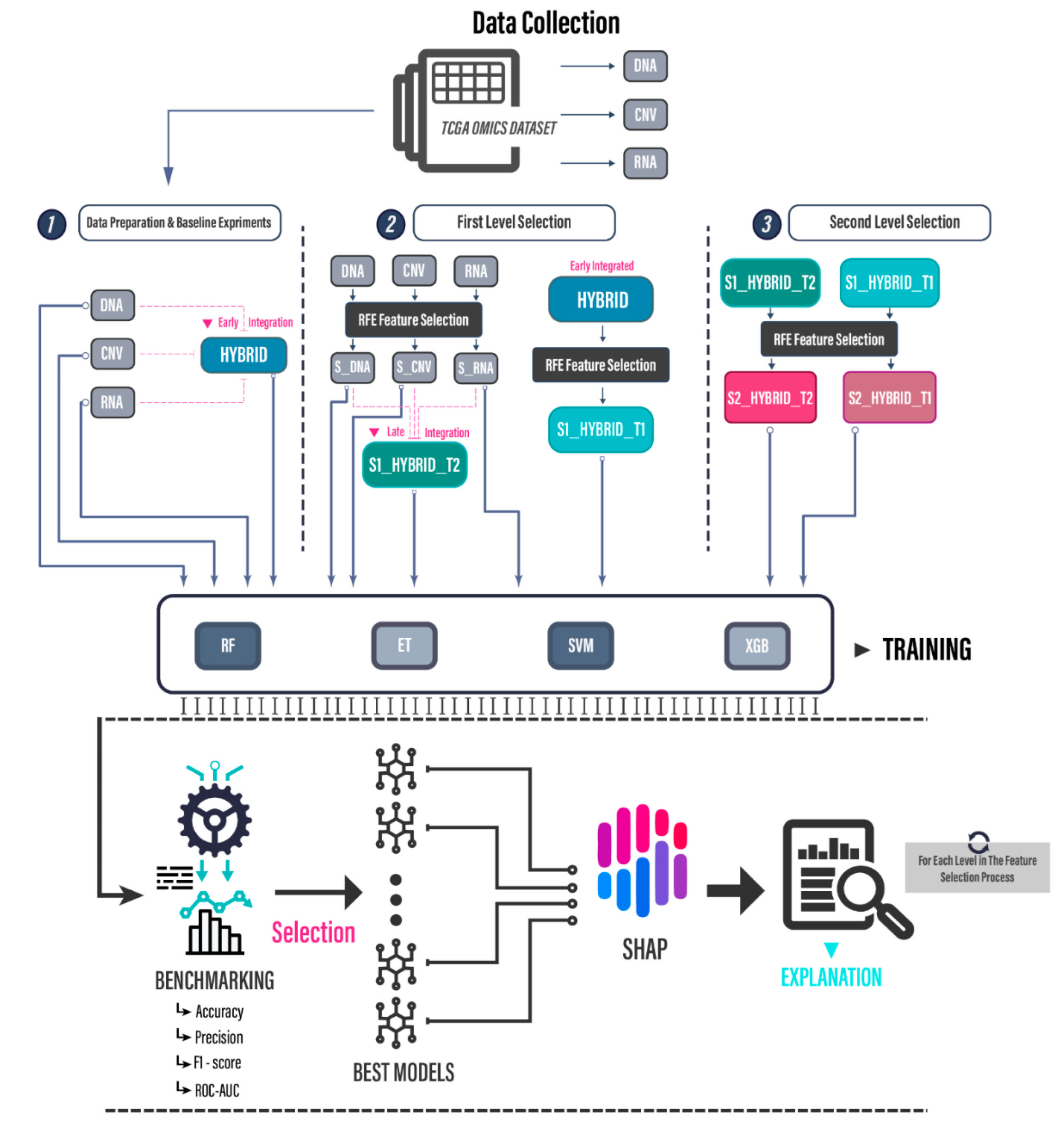
To address the aforementioned issues, we propose a multi-stage feature selection framework for dimensionality reduction in a multi-omics context and then investigate the impact of the selected features on breast cancer subtype prediction. Figure 1 illustrates the proposed framework. This approach extends our previous study [25] by focusing on improving the multiclass classification task which requires the accurate identification of five subtypes and by taking an additional step toward interpretability, which aims to provide greater insight into the data and the algorithms.

As part of this framework, we consider the TCGA omics dataset, which, as previously stated, contains many features and modalities. Another motivation is to establish a testing benchmark against which we can compare our results to state-of-the art studies.

Considering this, we intend to develop a model that can accurately predict five cancer subtypes while also remaining highly interpretable for future research. The study utilizes three distinct data types, DNA methylation, CNV, and mRNA descriptors (for short, we will refer to them as DNA, CNV, and RNA, respectively, in the rest of the paper), as well as a two-stage feature selection approach with multiple data integration strategies. The process begins by establishing a benchmark against which we monitor the prediction progress. This is achieved by integrating the data from the three sources into one dataset named as HYBRID in Figure 1. After feeding the data to the machine learning fine-tuned models, the results are computed using a cross-validation procedure. In the multi-step feature selection process that follows, feature selection is applied, new datasets are generated, and benchmark reports are compiled. At each stage, each set of features is individually and collectively analyzed based on SHAP interpretation to determine the significance of each feature, the impact of their fusion, and how their fusion technique affects the classification task.

Figure 1, therefore, depicts four key informational elements: the datasets used, the feature selection algorithm, the integration schemes, and the machine learning models. The following will elaborate on these components.

3.1. Datasets and Integration Schemes

The datasets used in this study are from TCGA. Similar to [16,17], the datasets used cover 3 types of modalities, including 13,195 mRNA features, 14,285 DNA methylation features, and 15,186 unique CNV features. In total, 606 cases were recorded in the datasets and were classified into 5 categories based on the ER, PR, and HER markers, as described in the two aforementioned works: luminal A, luminal B, ERBB2 (HER2(+)), TNBC, and Unclear, with 277, 40, 11, 70, and 208 instances, respectively.

Using feature selection and different integration schemes, the following datasets have been generated from these three original datasets:

• HYBRID: this dataset is the result of combining the three original datasets, yielding a 46,666 × 606 dataset.
• S_DNA, S_RNA, and S_CNV: these datasets are obtained by individually selecting features from each dataset.
• S1_HYBRID_T1 (S1HT1): this dataset is derived using selected features from HYRID dataset.
• S1_HYBRID_T2(S1HT2): this dataset is derived by combining the S_DNA, S_RNA, and S_CNV datasets.
• S2_HYBRID_T1(S2HT1): this dataset is derived from S1_HYBRID_T1 using the selected features.
• S2_HYBRID_T2(S2HT2): this dataset is derived from S1_HYBRID_T2 using the selected features.

3.2. Feature Selection Algorithm

As a means of reducing dimensionality and improving our model’s efficiency even further, we resorted to feature selection. Feature selection (FS) is considered one of the most important pre-processing tasks in a machine learning life cycle as it enables the process to cope with the curse of dimensionality and properly handle the so-called large p, small n problems.

This process enables us to reduce computational complexity and, in some instances, filtering irrelevant and redundant features while maintaining the overall integrity of the dataset, which consequently, in certain situations, enhances the classification performance.

This stage is required in our study as we want to identify the most essential features and use that subset to increase the classification performance of the models while also being able to explain the logic behind the outcomes. Thus, in this research we enforced the interpretability aspect by relying on feature selection techniques.

Several techniques of feature selection exist, which can be grouped into 3 main categories: filter, wrapper, and embedded methods, each with its advantages and disadvantages.

Filter methods [26,27] are based on the principle of rank and pruning. They make use of heuristic rules to evaluate features’ predictiveness based on intrinsic data properties. The wrapper approach [26,27] evaluates the subset of features as a potential indicator of the model’s performance. This method requires a predetermined learning algorithm and uses the performance of the learning algorithm to determine which features are selected. The embedded approach [27], which is a compromise between rank and wrapper and incorporates feature selection into the learning method. Therefore, it can inherit the advantages of filter and wrapper approaches.

As the goal is to improve model performance rather than computation efficiency, we chose recursive feature elimination [28] as the FS technique. Despite its greedy nature, it is widely used for feature selection as it is relatively effective and efficient in reducing model complexity by removing irrelevant features.

As the name suggests, RFE works by removing features recursively and then building a model on the features that remain. It is a wrapper method that internally employs filter-based feature selection. RFE ranks features by importance and calculates accuracy by evaluating smaller subsets of features recursively. Such a method requires a ranking algorithm for features. Model accuracy is used to determine which features (and combinations of features) contribute the most to accurately predicting the target class. This technique starts by creating a model with all of the features in a given set and assigning an importance score to each feature. Then, one by one, the least important feature(s) are removed from the current set of features and importance scores are computed again, until we are eventually left with the desired subset of features. To score features, the provided machine learning model is used. To estimate the importance of features, bagged decision trees such as random forest and extra trees can be used. After several attempts to optimize the process, we resorted to the random forest algorithm. This allowed us to have a more complete overview of the subsets of features. More formally, a simplified version of RFE can be described as shown in Algorithm 1 below:

Algorithm 1 Recursive Feature Elimination (RFE)

Inputs: A set of features S = {fi, i = 1…n} A classifier model M (random forest or extra trees) A training dataset X A target variable y The desired number of features Nbest

1: while (size(S) > Nbest) do 2:   Fit the model M on the dataset restricted to good features S: 3:       Ms = train_model (X(S), y) 4:   Rank the features in S according to their importance using the model Ms 5:       Sranked = rank (S, features_importance(Ms)) 6:   Remove the least important feature fi: 7:       S = Sranked − {fi} 8: end while 9: Sbest = S

Output: the selected subset of features Sbest

3.3. Machine Learning Models

We initially investigated a variety of traditional and ensemble algorithms in preliminary experiments, all of which were fine-tuned accordingly using Grid Search. The most performant and consistent algorithms were chosen based on our findings and those of the literature. In addition, for further interpretability, we selected algorithms with different approaches to a classification task. The following will briefly describe the selected algorithms.

3.3.1. Support Vector Machine

The support vector machine (SVM) is a well-known machine learning algorithm that was originally developed to solve supervised learning problems by Vapnick et al. [29]. SVM has grown in popularity as a result of its superior generalization ability and successful applications. A comprehensive survey on SVM models is given in [30]. Despite the widespread adoption of deep learning models, SVM remains a viable option for many issues where deep learning cannot be successfully applied, especially when sufficiently big datasets are unavailable [31]. SVM is primarily based on the class separation principle. It seeks to identify support vector instances that lie along the margin extents in order to find the largest margin between classes. The decision boundaries for the classes are defined by the support vectors, which are critical instances. As a result, training a support vector machine for linearly separable instances looks specifically for the best separating hyper-plane with the greatest margin between the different data points. SVM, on the other hand, maps non-linearly separated data instances into higher dimensional space where the data can be separated linearly. Kernels are similarity functions that support dot products with special properties that allow a function to be substituted for a higher dimension space. Many kernel functions are supported by SVM, including linear kernel, polynomial kernel, and radial basis kernel. SVM has also been extended to handle unsupervised learning problems.

Formally, training a SVM model is performed by solving the following quadratic and convex problem optimizing the following quadratic objective function:

$$mi{n}_{w,b,\xi }\frac{1}{2}\Vert w^2\Vert +C{\displaystyle \sum }_i{\xi }_i$$

subject to

$$y_i\left(\langle w,\phi (x_i)\rangle +b\right)\ge 1-{\xi }_i and {\xi }_i\ge 0$$

where:

• φ(·) is the feature map corresponding to some kernels;
• (w, b) are the parameters of the separating hyperplane with $w\in {ℝ}^n \mathrm{and} b\in ℝ$;
• $x_i$ refers to the data point;
• $y_i\in \left\{-1,1\right\}$ is the data point label;
• ${\xi }_i$ is a slack variable that represents the impact of the misclassified data;
• $C$ is a penalty term.

3.3.2. Ensemble Learning

It is well known that there is no algorithm that is always the most accurate, according to the no free lunch theorem. Rather than relying on a single model, combining the advantages of multiple models has the potential to mitigate the weaknesses of each individual model. The resulting combined model ought to be more robust and less error-prone than any individual model. This is called ensemble learning, which is prevalent in machine learning and statistics. Multiple machine learning models’ decisions are combined to minimize errors and achieve aggregated decisions that enhance prediction. Each classifier is weak but the ensemble is strong. Ensemble learning systems have proven to be highly effective and extremely versatile across a variety of problem domains and real-world applications [32].

Ensembles can be created in a variety of ways. Simple ensembles use voting or averaging predictions of multiple pre-trained models. Another approach of ensembles consists in training the same model multiple times on different datasets and combine these different models rather than training different models on same data. Simple (weak) models can be used as the base models. Bagging (parallel ensemble) [33,34] and boosting [34,35,36] (sequential ensemble) are two methods for performing ensemble learning. Representatives from each class have been considered in our work.

Bagging entails taking repeated bootstrap samples from the training dataset and training a different classifier on each sample in parallel. Bootstrapping is the first step in the bagging process flow, in which the data is divided into randomized samples. Following that, classifiers are trained in parallel with these randomized samples. Bagging makes predictions based on the majority vote or the average. Random forest and extra trees are two examples of bagging ensembles.

Random forests [37] are ensemble learning methods designed specifically for decision tree classifiers. They are based on two randomness sources: bagging and subspace sampling. The process of growing each tree using a bootstrap sample of training is referred to as bagging. The latter only uses a randomly selected subset of the descriptive features in the dataset, which is referred to as subspace sampling. Random forest makes predictions by returning majority vote or median value.

The extra tree, also known as the extremely randomized tree [38], is a model similar to decision trees and random forests, but it uses additional data information to enhance predictive accuracy. It is very similar to random forest but it uses a different method to construct the decision trees. Random forest uses bootstrap replicas (bootstrapping), whereas extra tree uses the entire original dataset. Another distinction is the choice of cut points for splitting nodes. Random forest selects the best split, whereas extra tree selects it at random. However, once the split points are determined, the two algorithms determine the best one among all the feature subsets. As a result, extra trees introduces randomization while maintaining optimization.

Boosting is a sequential ensemble learning technique for improving the accuracy of a model by transforming a weak hypothesis or weak learners into strong learners. Boosting trains classifiers sequentially (e.g., decision trees). A new classifier should focus on those cases, which were misclassified in the previous round. It combines the classifiers by letting them vote on the final prediction (like bagging).

The boosting algorithm generates new weak learners (models) and combines their predictions sequentially to enhance the model’s overall performance. It performs by assigning larger weights to misclassified samples and lower weights to correctly classified samples. Weak learner models with higher performance are given more weight in the final ensemble model. AdaBoost was the first boosting implementation (adaptive boosting). Gradient boosting is a type of boosting algorithm in which errors are minimized using a gradient descent algorithm and a model in the form of weak prediction models, such as decision trees, is produced. Gradient boosting has been improved in terms of computational speed and model performance and scaled to extreme gradient boosting (XGBoost) [39], which is the most widely used public domain software for boosting.

3.4. Shapley Additives Explanations Framework

Explainable Artificial Intelligence, or XAI, is the process of understanding the reasoning behind the model’s results and why and how inquiries are related to those outcomes, while also allowing visibility into how these algorithms function at each stage of their problem-solving approach [40].

Considering the tradeoff between performance and interpretability, we considered a popular XAI framework based on game-theory known as SHAP (Shapley additive explanations). This framework can be used to explain the outcomes of different AI models and different forms of datasets by figuring out the best way to give out credit to local explanations using the traditional Shapley values and extensions of game theory [41]. SHAP itself assigns a significance value, or SHAP Value, to each characteristic in each prediction. Each value describes how to get from an expected base value to an observed output if we had no information about the current output [41]. These values provide a one-of-a-kind additive feature significance measure that satisfies all three properties of local accuracy, missingness, and consistency while defining simplified inputs using conditional expectations [41]. The SHAP method approximates these values utilizing six alternative methods, two of which are model-agnostic while the other four are model-type-specific. An in-depth and exact explanation by which the values are calculated can be quite lengthy and is out of scope of this work, therefore we recommend reviewing the proposed framework on the original paper [41].

4. Experimental Study and Results

A comprehensive experimental study was carried out. For the sake of clarity and to provide a concise and precise description of the experimental results, their interpretation, and the experimental conclusions that can be drawn, we organize this section as follows:

First, we describe the test environment, including the hardware and software used for implementation, and then we discuss the performance metrics we used to benchmark our results. The results are then presented and discussed.

4.1. Implementation Environment

The experimental environment’s hardware consists of a 3.4 GHz 16-core Ryzen 9 5950X processor, 32 GB of RAM, and an Nvidia RTX 3080 TI. In terms of software, and in efforts to adhere to the FAIR Guiding Principles of reusability and data management [34], we implemented the classification models using Python 3.8 with the scikit learn package version 0.23.2 and fine-tuned the models using Grid Search. More details concerning the parameters’ settings can be found on GitHub [42]. Later, the SHAP package version 0.40.0 was used for classification interpretation. The code can be found on GitHub [42].

4.2. Performance Metrics

As mentioned earlier, the target feature has five levels: luminal A, luminal B, ERBB2(HER2(+)), TNBC, and Unclear. Therefore, the confusion matrix corresponding to the multiclass classification is a 5 × 5 matrix. Based on the one-versus-rest strategy, true positive (TP), true negative (TN), false positive (FP), and false negative (FN) are defined. The following performance metrics are used to assess the performance of the various proposed models using the selected features and integration schemes. These measures are derived from the confusion matrix as follows:

Accuracy: This measure gives the rate of instances correctly classified (ICC) among all test instances (TI). Let us denote through ${\mathrm{N}}_{\mathrm{ICC}}$ and ${\mathrm{N}}_{\mathrm{TI}}$, the numbers of ICC and TI, respectively. The accuracy can be defined as:

$$\mathrm{Accuracy}=\frac{{\mathrm{N}}_{\mathrm{ICC}}}{{\mathrm{N}}_{\mathrm{TI}}}$$

Precision: Precision refers to the proportion of predicted positive instances that are in fact positive. Therefore, for each of the five previously mentioned classes, precision represents the classifier’s ability to predict the type of BC in a patient with that type of BC, i.e., luminal A. Increasing precision decreases false positives and increases true positives. For each level or class, precision is defined as:

$$\mathrm{Precison}\left(\mathrm{i}\right)=\frac{\mathrm{TP}\left(\mathrm{i}\right)}{\mathrm{TP}\left(\mathrm{i}\right)+\mathrm{FP}\left(\mathrm{i}\right)} \mathrm{i}=1\dots 5$$

The overall precision is the average over all classes.

Recall: This metric, also known as sensitivity, measures the proportion of actual positive instances that are predicted as positive. Therefore, for each of the five classes previously mentioned, the recall metric indicates the classifier’s ability to find all instances with that class. Improving recall reduces false negatives and increases true positives. For each level or class, recall is defined as:

$$\mathrm{Recall}\left(\mathrm{i}\right)=\frac{\mathrm{TP}\left(\mathrm{i}\right)}{\mathrm{TP}\left(\mathrm{i}\right)+\mathrm{FN}\left(\mathrm{i}\right)} \mathrm{i}=1\dots 5$$

The overall recall is the average over all classes.

F1-score: In case of class imbalance, F1-measure (or F1 score) is a more reliable measure to assess the performance of the classification. It concentrates on minimizing both false positives and false negatives. It is the harmonic mean of precision and recall and can be defined as follows:

$$\mathrm{F}1 \mathrm{score}=2\frac{\mathrm{Precision}\ast \mathrm{Recall}}{\mathrm{Precision}+\mathrm{Recall}}$$

where Precision and Recall are the average over the precision and recall for each class.

$$\mathrm{Precision}={\displaystyle \sum }_{\mathrm{i}=1}^{\mathrm{i}=5}\mathrm{Precision}\left(\mathrm{i}\right) \mathrm{and} \mathrm{Recall}={\displaystyle \sum }_{\mathrm{i}=1}^{\mathrm{i}=5}\mathrm{Recall}\left(\mathrm{i}\right)$$

(1)

ROC_AUC: The receiver operating characteristics (ROC) curve is a probability curve that is used to evaluate the performance of classification models with varying threshold settings. It demonstrates the model’s ability to distinguish between classes. The area under the curve (AUC) is used to quantify this separability ability. The greater the AUC (close to 1), the better the performance and ability to differentiate between classes. When the AUC is close to 0.5, it indicates an inability to differentiate between classes. When AUC is close to 0, the model tends to invert the classes.

4.3. Experiments and Results

The experimental results will be presented according to the workflow depicted in Figure 1. First, we will describe the experiments that were carried out using the baseline datasets and the hybrid datasets obtained during the early integration. The first-level feature selection experiments’ results will then be discussed and different integration schemes will be evaluated. After that, the results of the second level feature selection experiments will be presented and discussed with further interpretation. The obtained results will be compared to those of other techniques described in the literature. The impact of the features on classification will also be discussed.

4.3.1. Baseline Experiments

Initial experiments consist of benchmarking our fine-tuned models on the three original datasets and the HYBRID dataset. During the preparation process, labels were encoded, and the dataset was transformed into a format compatible with our fine-tuned models.

Table 1. DNA Raw Experimental Results.

Classifiers	Accuracy	Precision	Recall	F1-Score	ROC_AUC
Random Forest	74.112	68.416	74.112	70.542	86.209
Extra Trees	74.604	68.753	74.604	71.069	85.046
SVM	56.940	44.975	56.940	49.753	80.191
XGBoost	76.913	73.695	76.913	74.502	88.683
AVG	70.6420765			66.467

,

Table 2. RNA Raw Experimental Results.

Classifiers	Accuracy	Precision	Recall	F1-Score	ROC_AUC
Random Forest	61.249	58.381	61.249	58.512	80.589
Extra Trees	61.243	59.426	61.243	57.936	81.821
SVM	56.273	52.602	56.273	51.138	81.975
XGBoost	63.227	61.740	63.227	61.647	82.565
AVG	60.49795082			57.308

and

Table 3. CNV Raw Experimental Results.

Classifiers	Accuracy	Precision	Recall	F1-Score	ROC_AUC
Random Forest	61.907	58.049	61.907	58.734	81.741
Extra Trees	58.451	55.331	58.451	55.235	81.473
SVM	56.273	52.602	56.273	51.138	81.975
XGBoost	63.227	61.740	63.227	61.647	82.565
AVG	59.96448087			56.689

show the results, while Figure 2 provides a summary.

Analyzing these tables reveals a substantial disparity in classification results based on modality. This raises the question of whether certain modalities are more suited to this classification task than others, and if so, which modalities are more suited to this task. In addition, which set of features is most important for each modality?

Based on these baseline results, a significantly higher classification rate has been achieved by relying solely on DNA features, as we observed an increase in approximately 10% in both f1-score and accuracy results when compared to other modalities. Moreover, while the focus of this research study is on the data rather than presenting a novel machine learning model, evaluating the models enables us to fine-tune the subsequent iterations and to understand how the data influences the model’s overall efficiency. Consequently, we can see that ensemble learners are consistently able to attain the highest scores.

In addition, we conducted a second baseline test with the HYBRID dataset, which was obtained by integrating the original three datasets early on. The objective is to confirm or refute the hypothesis that combining diverse data sources can significantly improve the overall performance of the model in this particular case, as has been explored in [24,43]. The results are presented in

Table 4. HYBRID Raw Experimental Results.

Classifiers	Accuracy	Precision	Recall	F1	ROC_AUC
Random Forest	77.577	76.305	77.577	75.531	92.313
Extra Trees	78.066	74.444	78.066	75.128	92.280
SVM	56.590	51.747	56.590	47.161	88.830
XGBoost	79.885	80.101	79.885	79.194	92.438
AVG	71.35063752			69.254

and Figure 2.

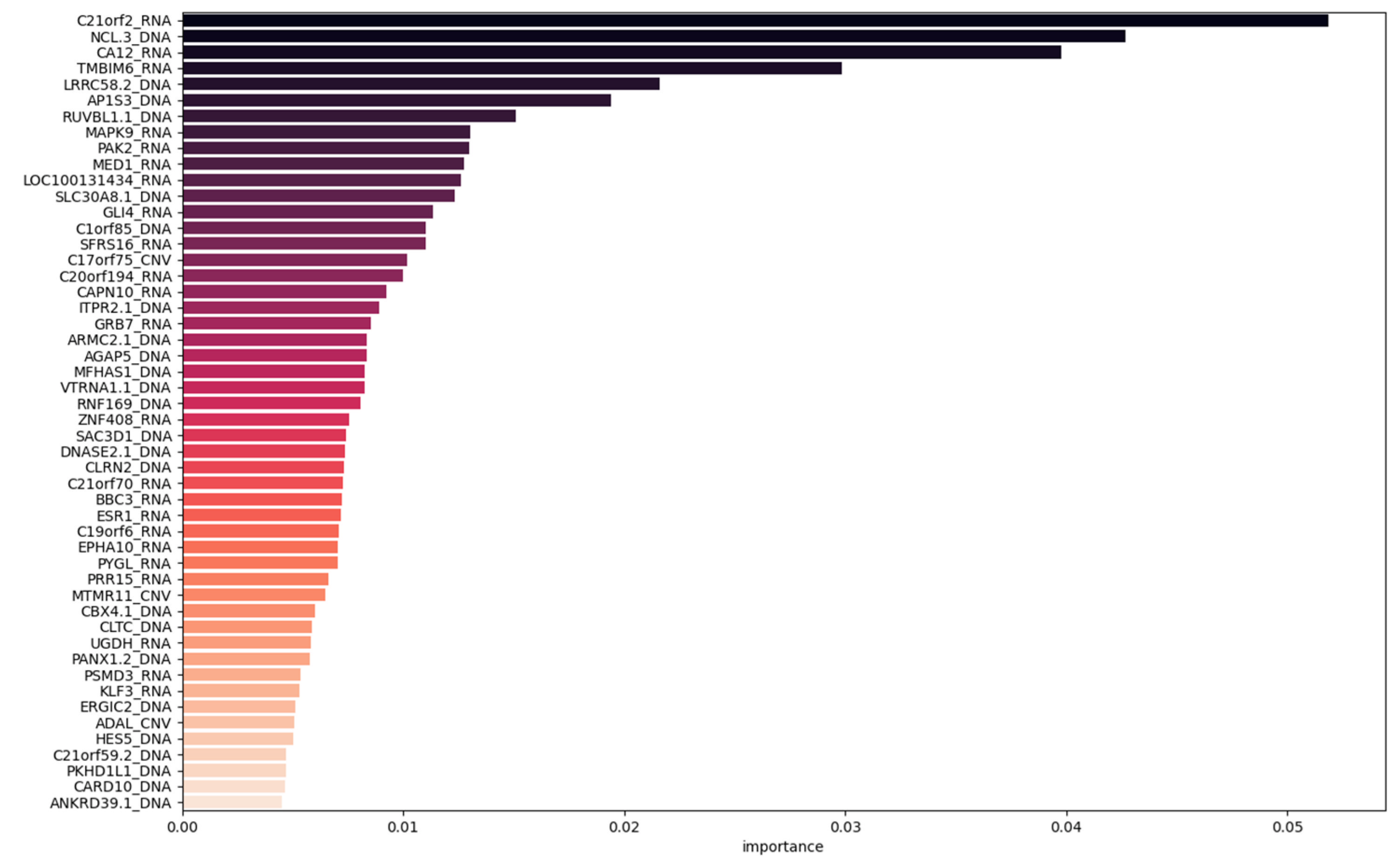
As expected, by combining all features, we were able to increase the classification rate against mRNA and CNV datasets by approximately 15% and by approximately 3% compared to the previous best models. To gain a deeper understanding of this behavior, we will interpret the classification process using information gain based on the best model, XGBoost in this case. As can be seen on Figure 3, we found 48% DNA features, 46% mRNA features, and only 6% CNV features among the top 50 important XGBoost features. With cumulative weights of 0.47, 0.48, and 0.04, respectively, across the entire dataset. This was expected, given that models employing DNA features solely had higher detection rates, and thus a greater contribution to the hybrid set was expected.

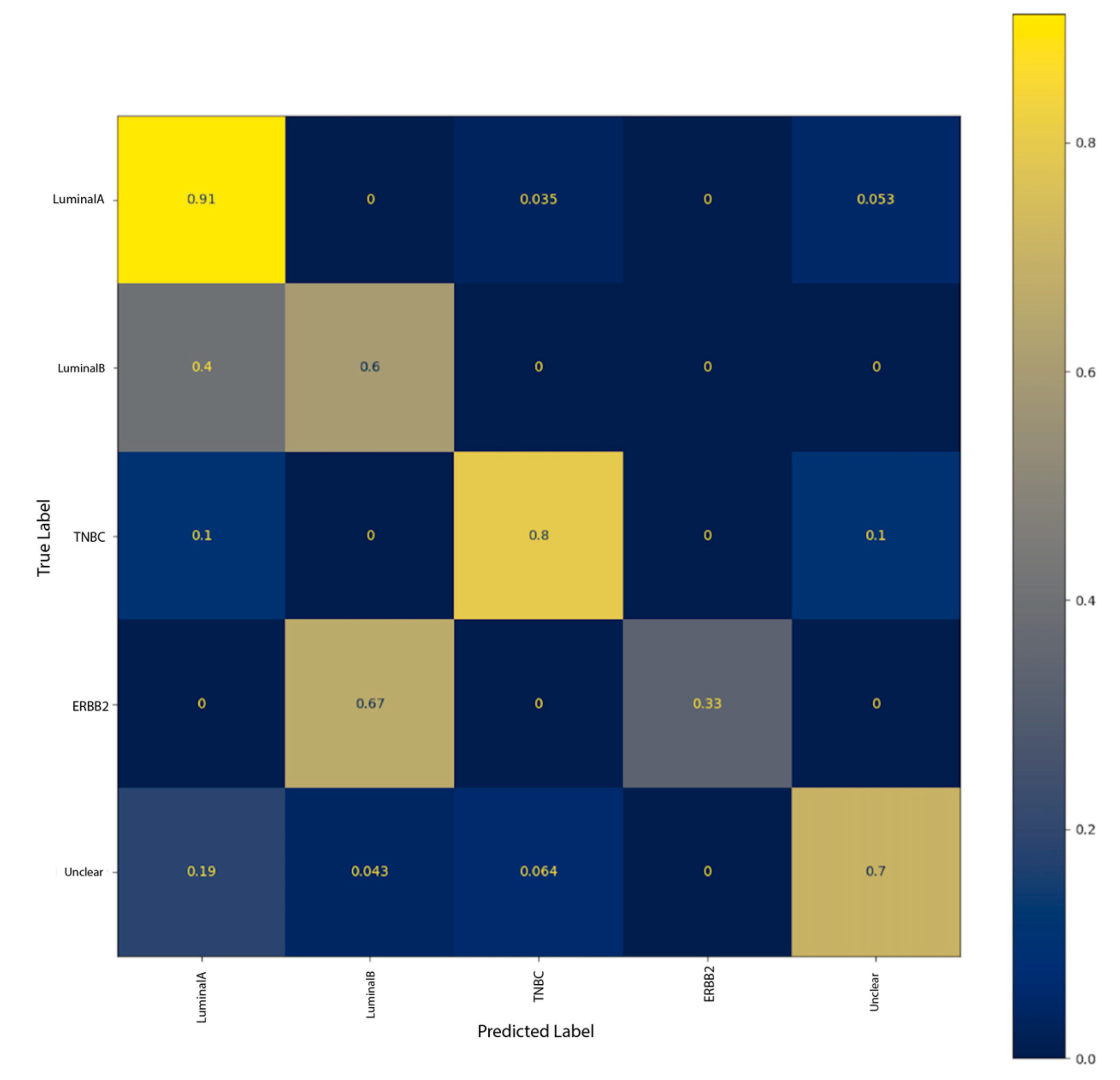
This behavior can be interpreted in greater detail using the normalized confusion matrix (Figure 4) according to the true labels and SHAP summary plots (Figure 5) which will help us understand the nature of the contribution made by each set of features. SHAP plots make it easier to see how the features affect the model’s predictions. Specifically, we can extract the most influential features based on mean SHAP values, as well as the magnitude of each feature to the classification process, using the summary plot.

As shown in the normalized confusion matrix in Figure 4, the best performing model using the Hybrid dataset performs better at classifying luminal A and Unclear instances. Some TNBC instances were wrongly classified as luminal A and Unclear. Additionally, most of luminal B instances were classified as luminal A and all ERBB2 instances in the test set were classified as luminal B.

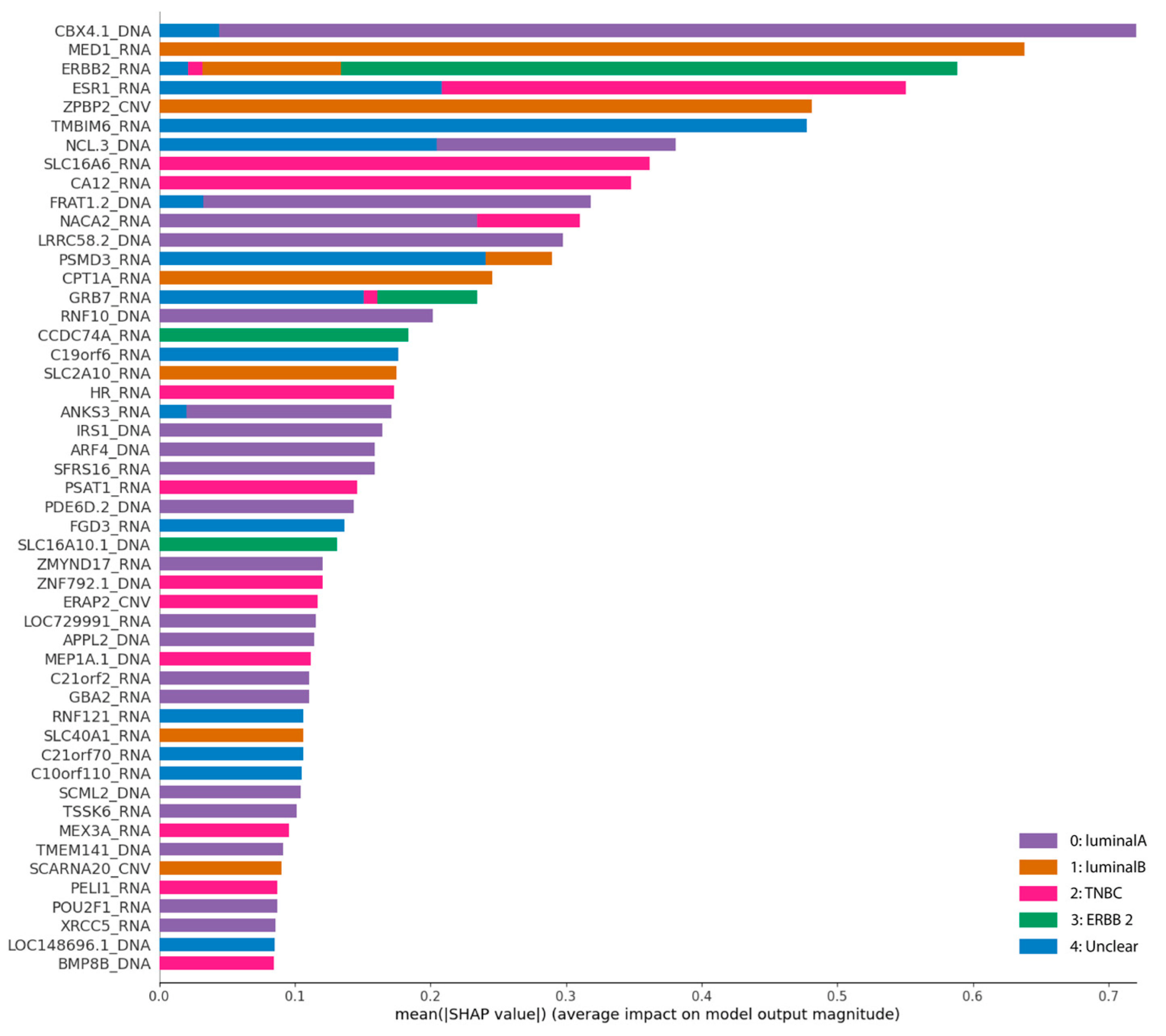
The SHAP summary plot of the classification process using the Hybrid dataset and the XGBoost classifier is shown in Figure 5. This graph ranks the features in descending order based on their influence on the model’s predictions by computing the mean SHAP values for each variable. Because we are dealing with a multiclass classification task in our scenario, the summary plot ranks the features based on their overall contribution to all classes and color codes the magnitude for each class. The mean threshold in our example was determined programmatically, allowing us to identify the top 50 most influential features.

In Figure 5, we can see at a glance that RNA and DNA features have a significant impact on the classification process, as depicted in the SHAP summary plot displayed below. RNA and DNA features have the greatest influence on luminal A, luminal B and ERBB2 (HER2 (+)) and TNBC subtypes, whereas CNV has a greater impact on luminal B and TNBC classification instances. The Unclear class, on the other hand, is primarily influenced by RNA and DNA features.

Before delving further into the interpretation of the results, we preferred to enhance accuracy rates and address concerns regarding the high feature dimensionality and limited sample presence. Consequently, the subsequent experiments will elaborate on the selection of the most useful feature subsets as well as strategies to improve classification rates and, ultimately, a more accurate interpretation.

4.3.2. Level 1 Experiments

This stage’s objective is to reduce the dimensionality of the baseline datasets as much as possible, while simultaneously improving performance and preserving the integrity and interpretability of our data. As previously described, RFE was used to classify features into subsets belonging to classes ranging from 1 to n, with class 1 being the most significant. As depicted in Figure 1, the resulting subsets are constructed from class 1 features and subsequently fused into a hybrid dataset using two distinct strategies.

In the first approach “T1”, the subset is derived directly from the original hybrid dataset, where we achieved the highest scores, whereas in the second approach “T2”, we take a late integration approach in which we extract the optimal subsets from each individual descriptor and then combine them into a single dataset. The subsequent fine-tuned models performed as shown in the

Table 5. Experimental Results using S_DNA with 1085 features.

Classifiers	Accuracy	Precision	Recall	F1	ROC_AUC
Random Forest	76.751	71.156	76.751	73.254	91.258
Extra Trees	76.743	71.149	76.743	73.261	90.298
SVM	63.544	58.916	63.544	58.919	85.704
XGBoost	78.402	75.862	78.402	76.303	90.996
AVG	73.860

,

Table 6. Experimental Results using S_RNA with 1586 features.

Classifiers	Accuracy	Precision	Recall	F1	ROC_AUC
Random Forest	63.874	61.690	63.874	61.908	84.850
Extra Trees	65.691	64.618	65.691	63.549	85.153
SVM	61.574	60.500	61.574	58.893	84.716
XGBoost	63.391	61.709	63.391	61.581	83.699
AVG	63.633

,

Table 7. Experimental Results using S_CNV 486 features.

Classifiers	Accuracy	Precision	Recall	F1	ROC_AUC
Random Forest	66.189	65.329	66.189	64.490	86.606
Extra Trees	67.516	66.496	67.516	65.746	86.318
SVM	61.577	60.379	61.577	58.163	84.291
XGBoost	64.880	64.244	64.880	63.438	84.707
AVG	65.040

,

Table 8. Experimental Results using S1HT1 with 166 features.

Classifiers	Accuracy	Precision	Recall	F1	ROC_AUC
Random Forest	83.669	84.029	83.669	83.338	95.346
Extra Trees	83.667	84.152	83.667	83.279	95.142
SVM	71.13934	68.01747	71.13934	67.24732	91.40257
XGBoost	83.003	83.737	83.003	82.742	94.097
AVG	79.270	78.594	79.270	77.776	93.615

and

Table 9. Experimental Results using S1HT2 with 3157 features.

Classifiers	Accuracy	Precision	Recall	F1	ROC_AUC
Random Forest	80.036	78.747	80.036	78.886	94.127
Extra Trees	80.858	79.940	80.858	79.798	93.459
SVM	63.844	62.392	63.844	61.173	86.633
XGBoost	79.041	79.613	79.041	78.594	93.051
AVG	74.307

below.

Starting with individual descriptors, using our strategy we were able to reduce the number of features in each dataset as seen in

Table 10. Shapes of produced datasets.

Reduction
Descriptor	Original Number of Features	New Set of Features	Reduction Percentage
DNA	14,285	1085	92%
RNA	13,195	1586	88%
CNV	15,186	486	97%

below.

After such extensive reshaping, not only were we able to preserve the dataset’s integrity, but we were also able to outperform the baseline scores in terms of accuracy by approximately 3%, while utilizing roughly 10% of the original datasets. We also achieved the highest scores using the hybrid dataset at this stage. By extracting directly from the original hybrid set, we were able to achieve significantly higher scores. As shown in the graph below (Figure 6), we observed a 5% increase in accuracy rates and a 4% increase in F1 scores compared to a late integration strategy.

One way to interpret these results is to study composition of these datasets. As shown in

Table 11. Composition of datasets.

S1HT1
Descriptor	Number of Features	Percentage
DNA	60	36%
RNA	89	54%
CNV	17	10%
Total	166
S1HT2
DNA	1085	34%
RNA	1586	50%
CNV	486	15%
Total	3157

, each percentage represents the proportion of features from the corresponding baseline dataset that contribute to the hybrid set under consideration. In S1HT1, for example, 36% of features are DNA features, 54% are RNA features, and 10% are CNV features.

Most features now originate from mRNA features, followed by DNA features, and finally a small subset of CNV features, as compared to the baseline set. According to our previous hypothesis, we would have expected DNA features to be more significant in accordance with the results obtained from individual datasets. However, the presence of more mRNA features indicates that these features had the greatest impact on classification and integration. To further analyze this behavior, a second level of feature extraction was considered for T1 and T2. Results revealed that features alone were unable to achieve high scores, but when combined, they did.

4.3.3. Level 2 Experiments

In this set, a second level of feature selection was conducted using RFE. The

Table 12. Experimental Results using S2HT1 with 118 features.

Classifiers	Accuracy	Precision	Recall	F1	ROC_AUC
Random Forest	84.000	84.361	84.000	83.624	95.032
Extra Trees	84.500	84.756	84.500	84.021	95.313
SVM	71.309	68.137	71.309	67.452	91.508
XGBoost	83.516	83.885	83.516	83.095	94.359
AVG	79.775

and

Table 13. Experimental Results using S2HT2 with 2388 features.

Classifiers	Accuracy	Precision	Recall	F1	ROC_AUC
Random Forest	80.533	79.280	80.533	79.502	93.929
Extra Trees	81.189	80.550	81.189	80.190	94.122
SVM	64.508	62.917	64.508	61.783	86.714
XGBoost	81.519	81.442	81.519	80.967	93.329
AVG	75.7386

below depict the results obtained in both T1 and T2 classification tasks.

In this second stage, the feature selection procedure iterated through each feature one at a time. We reduced 48 features from the T1 dataset and 769 from the T2 dataset, which is significantly less than the initial reduction rate. This indicates that, of the original 42,666 features, this dataset contains only the most influential and relevant features. We can also see that better performance has been achieved with S2HT1 dataset and extra trees model. In general, ensemble models perform better than SVM in all experiments.

A comparative study has been conducted using related works from the literature. Our results have been compared to those reported in [17] where the same datasets have been used. As we can see on Figure 7, we have in fact reached higher performance rates, not only in our experiments but also compared to the literature. We achieved an increase of 6.5% from the previous works in [17] in multiclass classification in terms of accuracy. As was achieved by our ensemble methods XGBoost and extra trees with a two-level feature extraction and an early integration approach to our different modalities.

Now, in an effort to improve interpretability, SHAP summary plots and the confusion matrix will be used. Both will be applied to the S2HT1 dataset, as we were able to obtain significantly higher classification rates using this set with the extra trees classifier.

The S2HT1 is composed of 45 DNA features, 60 mRNA features, and 13 CNV features, which only represent 0.27% of the original Hybrid dataset. The top 50 features (Figure 8) consist of 14 DNA features, 30 RNA features, and 6 CNV features with a global importance of 0.359 for DNA features, 0.528 for RNA features, and 0.113 for CNV features.

The graph (Figure 9) depicting the contribution of each feature to each class classification demonstrates a more balanced impact on all classes or subtypes. They influence the classification of every class to some extent, contrary to what has been observed in base experiments.

Besides confirming the high impact of the RNA features seen in the Figure 7, we can hardly understand the influence of each set features on the classification process. Hence, we breakdown this summary plot into individual plots per class accompanied by the confusion matrix as seen in Figure 10 below.

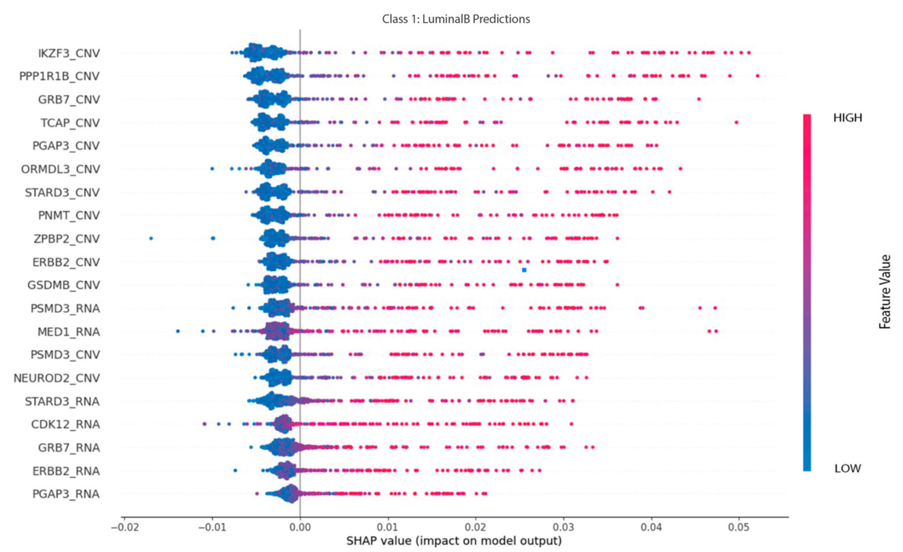
Figure 11 illustrates the impact of the features on the classification process in greater detail. This graph looks at the classification one class at a time. As a result, the important features on the Y-axis are ranked in descending order based on their impact on classification. The impact is depicted on the X-axis by the calculated SHAP value for each instance. If the SHAP value for an instance is positive (negative), it means that the corresponding feature has a positive (negative) impact on the classification for that instance. Each point on the summary plot is an instance, color-coded by a red-to-blue gradient representing the original value of the feature and positioned based on its distribution. The color red represents high values of the feature, while the color blue represents low values [44].

Figure 11 below shows that luminal A prediction is primarily influenced by DNA and RNA features. With ESR1, CA12, and CAPN10 as the top RNA features and CBX4.1 as the top DNA feature for this classification, we can observe that an increase in the values of RNA features indicates that the observed instance has a greater likelihood of being a luminal A subtype, while a decrease in the values of DNA features predicts the opposite.

On the other hand, as depicted on Figure 12, CNV features have a significant impact on the prediction of luminal B cases. These characteristics include IKZF3, PPP1R1B, and GRB7 as the most prominent for this subtype, with the likelihood of luminal B classification increasing as the value increases.

Regarding TNBC predictions, we can observe that only the most prominent mRNA characteristics, such as ESR1, CA12, MLPH, TBC1D9, and THSD4, have an impact on this classification. As the likelihood of a positive classification rises, the values of these features must decrease for a TNBC instance to be classified as such. As shown by the scatterplot in Figure 13, greater values of these characteristics are associated with a negative classification of this subtype.

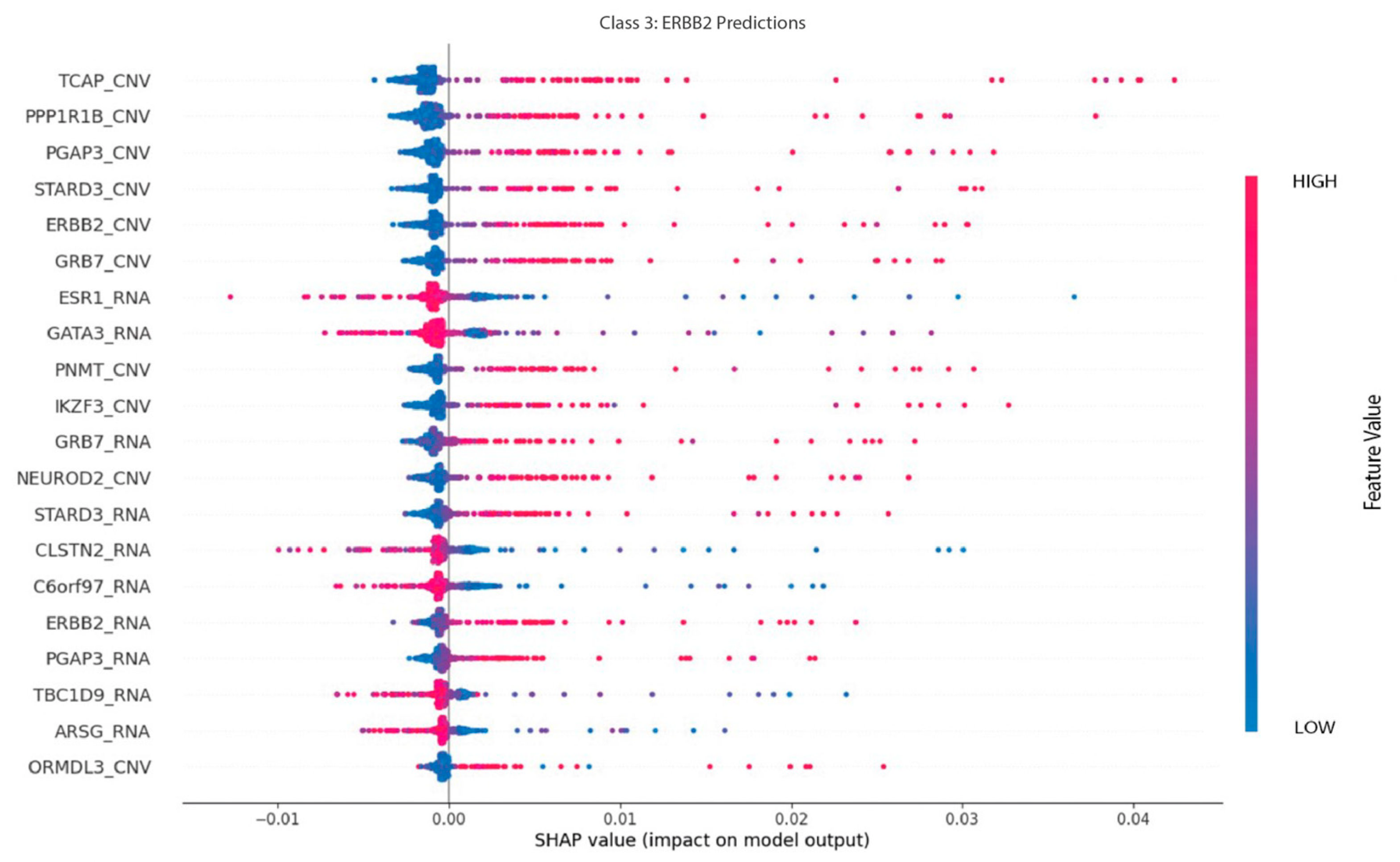
As shown in Figure 14, the main features regarding ERBB2 predictions are RNA and CNV features. TCAP, PPP1R1B, and PGAP are CNV features that positively influence this class prediction. RNA features, such as ESR1, GATA3, and CLSTN2, have a negative impact on this classification, however.

4.4. Results Summary

The best results obtained throughout the three steps of the proposed framework, as shown in Figure 1, are summarized in

Table 14. Results summary.

Integration–Selection Level	Best Model	Dataset	Results
Step 1: Baseline experiments with early integration.	XG-Boost	HYBRID (All features DNA, RNA and CNV)	Accuracy:	79.885%
			Precision:	80.101%
			Recall:	79.885%
			F1-score:	79.194%
			ROC-AUC:	92.438%
Step 2: First level feature selection with late integration.	Extra Trees	S1-HYBRID-T2 (Combining selected features from the three baseline datasets)	Accuracy:	80.858%
			Precision:	79.940%
			Recall:	80.858%
			F1-score:	79.798%
			ROC-AUC:	93.459%
Step 3: Second level selection	Extra Trees	S2-HYBRID-T1 (Features from HYBRID dataset after two level selection)	Accuracy:	84.500%
			Precision:	84.756%
			Recall:	84.500%
			F1-score:	84.021%
			ROC-AUC:	95.313%

. We can clearly see the benefit of performing several levels of feature integration and selection as results improve while progressing from one step to the next. The best results were achieved using the extra trees classifier with two levels of feature selection.

In our case, explaining why a model makes a particular prediction is just as important as the performance itself (in terms of the considered metrics). We used XAI methods, most notably SHAP, in this study to investigate the precise manner in which genomic data influence machine learning models in the classification of breast cancer subtypes. The main insights are summarized as follows:

-

First, by combining data with an early integration technique, the essential information for classification in the datasets was preserved, and the feature selection process was better optimized, resulting in an improve of the predictions. Additionally, ensemble methods were the most effective ML models for this type of classification with several classes, high dimension, a small number of instances, and imbalance in class distribution.

-

Using SHAP, we identified the most significant features according to their classification influence.

▪

Top DNA features include: NCL.3, CBX4.1, STK35, TMSB10, C17orf79, RNF10, FRAT1.2, PPP1R11, LRRC58.2, MPPE1.4.

▪

Top RNA features include: ESR1, CAPN10, NACA2, SNRNP70, CA12, C19orf6, PPP1R12C, TMBIM6, ANXA9, PPIAL4G, MAFK.

▪

Top CNV features include: PGAP3, GRB7, ERBB2, PNMT, NEUROD2, ZBP2, IKZF3, TCAP, ORMDL3, STARD3.

-

Furthermore, within the context of breast cancer subtyping, DNA and RNA characteristics were by far the most influential features. We observed that:

▪

Luminal A instances can be accurately identified when lower values of DNA features (including: CBX4.1, TMSB10, STK35), and Higher values of RNA features (including ESR1, CA12, GATA3) are measured.

▪

Luminal B may be correlated with an increase in the values of selected CNV characteristics, such as IKZF3, PPP1R1B, and GRB7, or with a similar pattern in RNA features, including PSMD3, MED1, and STARD3.

▪

mRNA features (including ESR1, CA12, MLPH, and TBC1D9) can be a leading sign of the presence of TNBC. We observed that a decrease in the values of specific RNA characteristics suggests the presence of the TNBC subtype, while the opposite is also true.

▪

On the other hand, ML models predominantly based on these three modalities DNA, RNA, and CNV struggle heavily in identifying ERBB2 instances. This can be related to the shortage in the ERBB2 instances.

Ultimately, we believe that in order to enhance further on this study, other modalities should be investigated or substituted (in the case of CNV features) or more instances regarding the minority classes should be provided.

5. Conclusions

The goal of this study was to improve the multiclassification performance of applied machine learning models for cancer subtyping. We used machine learning and data optimization techniques to approach this problem methodically. Our approach to data optimization is novel in that it combines a multi-stage feature selection with various data integration techniques all within an interpretable framework that can be used for future developments. We started by establishing a baseline benchmark against which we could achieve comparable results in the most recent state-of-the-art studies. The results obtained using individual and combined features were then analyzed. Later, we expanded on this foundation by concurrently interpreting the behavior of our proposed solutions and comprehending the impact of each set of features on the classification process. Using the SHAP interpretation, we explained the behavior of the machine learning classifiers. This is, to the best of our knowledge, the most comprehensive feature analysis of this dataset to date. In our interpretation, we looked at how different modalities, such as DNA, mRNA, and CNV features, contribute to the identification of a specific subset, which, to our knowledge, has not been investigated before. We were eventually able to identify the key features that influence the identification of each subset. Furthermore, several data integration methodologies were investigated, including early and late integration. Early integration with two levels feature selection using extra trees, on the other hand, achieved the highest classification rates. By the end of this study, the best model, extra trees with S2HT1 outperformed the results obtained in the literature when compared to DeepMO and MKL, with a 6.5% improvement. Moreover, this study further contributes to the interpretation of the investigated models and data while using a small subset of the original features.

As a result, we believe that this study can serve as a model for future datasets and cancer studies using machine learning approaches. The biological interpretation of the key findings is also planned for future work.