Numerical Solving Method for Jiles-Atherton Model and Influence Analysis of the Initial Magnetic Field on Hysteresis

Abstract

The Jiles-Atherton model was widely used in the description of the system with hysteresis, and the solution for the model was important for real-time and high-precision control. The secant method was used for solving anhysteretic magnetization and its initial values were optimized for faster convergence. Then, the Fourth Order Runge-Kutta method was employed to solve magnetization and the required computation cycles were supplied for stable results. Based on the solving method, the effect of the nonzero initial magnetic field on the magnetization was discussed, including the commonly used linear model of the square of magnetization under the medium initial value. From computations, the proposed secant iteration method, with supplied optimal initial values, greatly reduced the iterative steps compared to the fixed-point iteration. Combined with the Fourth Order Runge-Kutta method under more than three cycles of calculations, stable hysteresis results with controllable precisions were acquired. Adjusting the initial magnetic field changed the result of the magnetization, which was helpless to promote the amplitude or improve the symmetry of magnetization. Furthermore, the linear model of the square of magnetization was unacceptable for huge computational errors. The proposed numerical solving method can supply fast and high-precision solutions for the Jiles-Atherton model and provide a basis for the application scope of typical linear assumption.

1. Introduction

Hysteresis behavior exists widely in ferromagnetic materials and dynamic systems [1,2]. As complex nonlinear problems, the description, solution and control for the system with hysteresis have been widely studied in recent years. In regard to the hysteresis, there were two kinds of models, respectively named as physics-based and phenomenon-based models [3]. Based on the widely accepted micro-magnetism theory to explain the production of magnetic hysteresis, the physics-based model considered the magnetizing mechanism and most parameters in this kind of model to have certain physical means.

Among physics-based models, the Jiles-Atherton model [4,5,6,7,8] has been widely used on plenty of areas for its clear mechanism and high precision to describe the hysteresis character caused from materials, structures or motions [2,9,10,11,12,13,14,15,16,17,18,19,20,21,22]. In addition, the solving method has been directly given or indirectly mentioned. For the system response employing the Jiles-Atherton model, describing its hysteretic characteristic, solving the Jiles-Atherton model fast and accurately was the most important solving process, as other sub-models were generally formed by linear time-invariant system expressions. For solving the Jiles-Atherton model, the two approaches were roughly obeyed in engineering: (1) solving typical Jiles-Atherton expression directly; and (2) simplifying the typical Jiles-Atherton expression and solving the simplified expression.

For solving typical expression of the Jiles-Atherton model, Szewczyk and Michał Nowicki et al. [16,23,24] pointed out that no analytical solutions are available for the Jiles-Atherton model. Numerical integration or the Runge-Kutta method could be used for solving the model while the Riemann method may accumulate numerical errors during integrations. Li et al. [18] employed some fitting methods to compute the magnetization based on Jiles-Atherton model results. Fitting methods were quite helpful for fast solutions where the applicability was limited, while specified parameters that fitted functions were suitable to certain material. However, the errors were uncontrollable. Xue et al. [25,26] presented the fixed-point iteration method for solving anhysteretic magnetization. They mentioned that without enough iterative numbers, fixed-point iteration would reach low-precision results, especially under a low magnetic field. They employed Aitken and Steffensen methods and special functions as initial values to accelerate convergence, though the improvement was limited. Azzaoui et al. [27] described a generalization methodology for nonlinear magnetic field calculation, applied on two-dimensional finite volume geometry, by incorporating a Jiles-Atherton scalar hysteresis model based upon the definition of a modified governing equation derived from Maxwell’s equations. Perkkiö et al. [28] proposed a quasi-Newton method, namely a variant of the sparse Broyden’s method, to accelerate the solution of the nonlinear equation arising from the finite element method coupled with the Jiles–Atherton model. They pointed out the trade-off between the fast solution and stable convergence and their method was “engineering solutions” in the sense that the method was given without any mathematical proofs. Simone et al. [29] described and solved methods for hysteresis loops and dynamic energy losses in soft magnetic alloys by artificial neural networks. Based on the measured results divided into a training set and an assessing set, the model was effectively trained and then validated in the whole range of inductions and frequencies considered, which supplied a useful tool for future component design. Cristian et al. [30] also employed artificial neural networks for controlling the piezoelectric actuators with hysteresis loops. Combined with the Super-Twisting Algorithm, they enhanced the tracking accuracy more effectively than the traditional PID control method.

Besides solving typical expressions of the Jiles-Atherton model, Edmund Kokornaczyk et al. [31] and Xue et al. [25] proposed new functions instead of anhysteretic magnetization or irreversible magnetization expressions in the Jiles-Atherton model. Some researchers [32,33,34,35] constructed the linear time-invariant system model for the total system, with a magnetic hysteresis link, where the square of magnetization seemed to be in a linear relationship with the inputted magnetic field. These ideas were essentially mathematical approximations of complex functions in hysteresis models to avoid some physical or mathematical inconveniences; presented models were more easily solved than the typical expression of the Jiles-Atherton model. Furthermore, the 3D simulation method [36] could also be employed to solve the response of a complex system combined with a Jiles-Atherton type hysteresis.

Including nonlinear function, differential equation and sign functions, the Jiles-Atherton model was not so easily solved. The trade-off between high-precision and fast-algorithm always existed and a fast and high-precision solution was not easily reached. In addition, the commonly used linear assumption of the square of magnetization was not sufficiently verified. This paper employed the secant method for the solution of anhysteretic magnetization and verified that it has more efficiency than the fixed-point iteration method. Then, optimal initial values for the secant method were supplied for less iterative numbers. Based on anhysteretic magnetization, the magnetization was calculated by the Fourth Order Runge-Kutta method and the required computation cycles were supplied for stable results. The influences of different values of the initial magnetic fields on the results were discussed. Considering the magnetization was generally used in the square format for the subsequent model, the square of magnetization under the medium initial value was calculated and compared to the linear model to analyze the computational accuracy of linear assumptions. The proposed numerical method can supply fast calculation solutions for the Jiles-Atherton model with controllable accuracy, which is quite useful for future real-time, high-precision control of the system with hysteretic loop.

2. Revised Jiles–Atherton Model

The typical Jiles–Atherton model utilized five equations to describe the relationship between the external magnetic field H and total magnetization M. As a commonly used hysteresis model, the Jiles-Atherton model has been modified for many versions, which have different mathematical expressions in describing the magnetization. The inconsistencies were concentrated on three aspects [3,26]: the format of anhysteretic magnetization, energy conservation equation and the introduction of new sign function, respectively. Xue et al. [26] summarized these formats and presented one reasonable expression based on the mathematical properties of the used function and the practical change process of energy. Based on the revisions on the expression of M_an and the energy conservation equation, the model was written as

$$\{\begin{array}{l}{H}_e=H+\alpha M\\ M_{an}=M_s[\coth (\frac{H+\alpha M_{an}}{a})-\frac{a}{H+\alpha M_{an}}]\\ M=M_{irr}+M_{rev}\\ M_{rev}=c(M_{an}-M_{irr})\\ \frac{\mathrm{d}{M}_{irr}}{\mathrm{d}{H}_e}={\delta }_M\frac{M_{an}-M}{\delta k}\end{array}$$

(1)

where anhysteretic magnetization M_an, irreversible magnetization M_irr and reversible magnetization M_rev were three intermediate variables from the perspective of calculation. M_s is the saturation magnetization, α is the quantified domain interactions, a is the shape parameter for M_an, c is the reversibility coefficient and k is the average energy required to break pinning sites.

Two sign functions were used in the Jiles-Atherton model. δ is the sign function of the derivative of the magnetic field strength with respect to time, expressed by sign(dH/dt) and equal to 1 when dH/dt > 0 while −1 when dH/dt < 0. δ_M is employed to guarantee positive incremental susceptibilities and is expressed by sign{sign[(dH/dt)·(M_an − M)] + 1}. It is easily concluded that δ_M equals 0 under the condition of sign[(dH/dt)·(M_an − M)] < 0 and 1 under any other conditions.

3. Solution of M_an

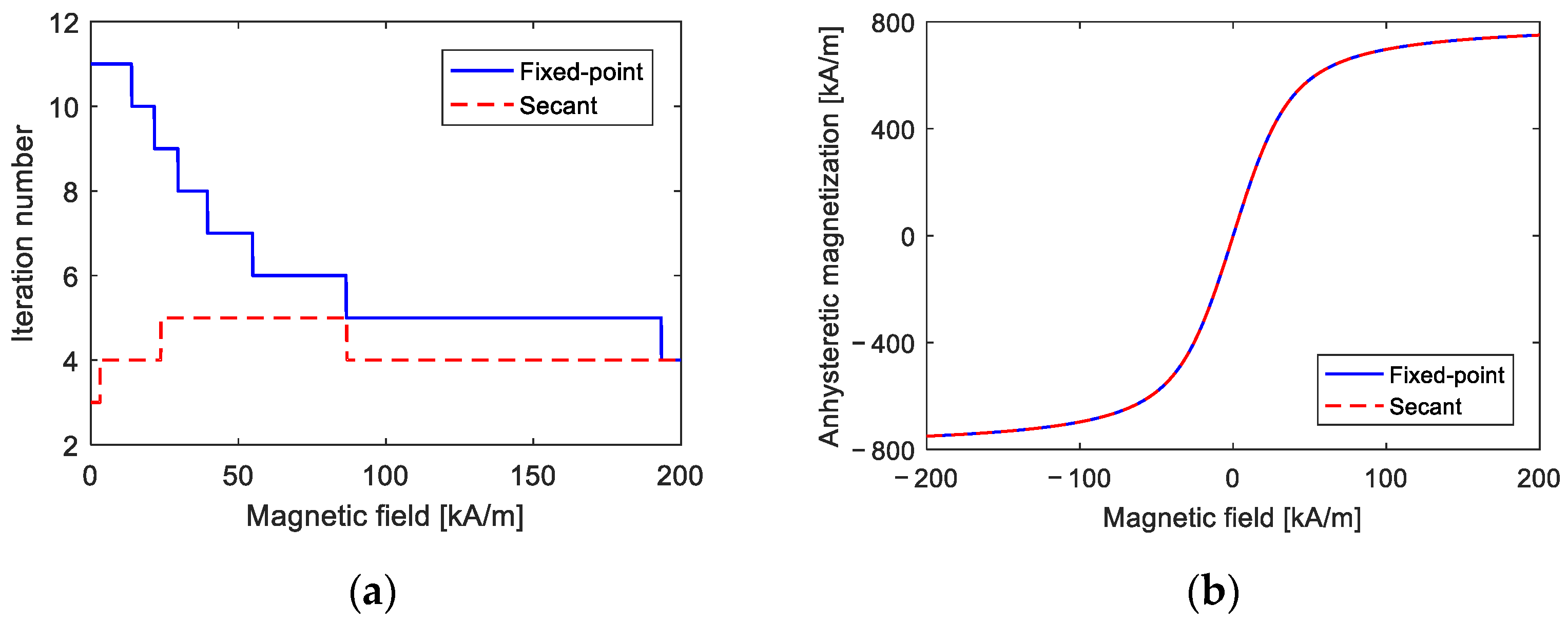
3.1. Secant Iteration Method

From Equation (1), the anhysteretic magnetization M_an can be reached directly from one equation of the revised Jiles–Atherton model as

$$M_{an}=M_s\left[\coth \left(\frac{H+\alpha M_{an}}{a}\right)-\frac{a}{H+\alpha M_{an}}\right]$$

(2)

Based on the right part of Equation (2), the global convergence of an iteration method can be reached. Impose g(M_an) = M_s{coth[(H + αM_an)/a] − a/(H + αM_an)} and then

$$\begin{array}{ll}\frac{\mathrm{d}g(M_{an})}{\mathrm{d}{M}_{an}}& =\frac{\alpha M_s}{a}\left[\frac{1}{{\left[\left(H+\alpha M_{an}\right)/a\right]}^2}-\frac{1}{{\sinh }^2\left[\left(H+\alpha M_{an}\right)/a\right]}\right]\\ & =\frac{\alpha M_s}{a}\left(\frac{1}{H_f^2}-\frac{1}{{\sinh }^2{H}_f}\right)\end{array}$$

(3)

where H_f = (H + αM_an)/a.

Considering the Taylor expansion of sinh H_f = H_f + H_f³/3! + H_f⁵/5! + …, dg(M_an)/dM_an is a monotonically decreasing positive function and meet

$$\begin{array}{ll}\frac{\mathrm{d}g(M_{an})}{\mathrm{d}{M}_{an}}& <\underset{H_f\to 0}{\lim }\frac{\alpha M_s}{a}\left(\frac{1}{H_f^2}-\frac{1}{{\sinh }^2{H}_f}\right)\\ & ={\underset{H_f\to 0}{\lim }\frac{\alpha M_s}{a}\left(\frac{{\sinh }^2{H}_f-H_f^2}{H_f^2{\sinh }^2{H}_f}\right)|}_{\mathrm{Lopida} \mathrm{rule} \mathrm{was} \mathrm{used} \mathrm{four} \mathrm{times}}\\ & =\underset{H_f\to 0}{\lim }\frac{\alpha M_s}{a}\left[\frac{4({\sinh }^2{H}_f+{\cosh }^2{H}_f)}{(4H_f^2+12)({\sinh }^2{H}_f+{\cosh }^2{H}_f)+32H_f\sinh H_f\cosh H_f}\right]\\ & =\frac{\alpha M_s}{3a}\end{array}$$

(4)

From Equation (3), the iterative method will be globally convergent as long as αM_s/a ≤ 3, which is satisfied in most cases. In fact, due to the rapid descent function 1/H_f²−1/sinh²H_f in the derivative expression, the iteration under αM_s/a > 3 is also convergent as long as the value of H is not too low (the solution can be set as 0 when H is too low). Under most conditions, dg(M_an)/dM_an is lower than 1; therefore, that arbitrary initial value will be convergent to the exact solution and the iteration based on the right part will show good sensitivity of initial value.

For the format of M_an, a natural function for the fixed-point iteration [37] was given as

$${M_{an(i+1)}^{}=M_s\left[\coth \left(\frac{H+\alpha M_{an(i)}^{}}{a}\right)-\frac{a}{H+\alpha M_{an(i)}^{}}\right]|}_{ M_{an(0)}^{}=0; i=0, 1, 2\dots }$$

(5)

where the subscript i is the iterative number, M_an(0) is the initial value of M_an and M_an(i) is the M_an value after i times of iterations.

Computing the time for the anhysteretic magnetization occupies most of the time of computing the magnetization as several numbers of calculations should be done on each value of the magnetic field. Saving the computing time of anhysteretic magnetization is the key to fast computation. The fixed-point iteration method was easily used, though inefficient, as the iteration numbers were really high. Even with the Aitken or Steffensen acceleration methods, the iterative duration was not reduced [26]. The tangent method or secant method has the advantages of fast convergence. Considering the derivative information of M_an was not given, the tangent method was not suitable, and the secant method was employed to reduce iterative numbers.

With the specified value of H as a known parameter, Equation (2) defines a nonlinear equation with an independent variable of M_an as

$$f(M_{an})=M_{an}-M_s\left[\coth \left(\frac{H+\alpha M_{an}}{a}\right)-\frac{a}{H+\alpha M_{an}}\right]=0$$

(6)

Then the secant iteration method can be used as

$$\begin{array}{ll}{M}_{an(i+1)}& =M_{an(i)}-\frac{f(M_{an(i)})\left(M_{an(i)}-M_{an(i-1)}\right)}{f(M_{an(i)})-f(M_{an(i-1)})}\\ & =M_{an(i)}-\frac{\left[\coth \left(\frac{H+\alpha M_{an(i)}}{a}\right)-\frac{a}{H+\alpha M_{an(i)}}\right]\left(M_{an(i)}-M_{an(i-1)}\right)}{\left[\begin{array}{l}\coth \left(\frac{H+\alpha M_{an(i)}}{a}\right)-\\ \frac{a}{H+\alpha M_{an(i)}}\end{array}\right]-\left[\begin{array}{l}\coth \left(\frac{H+\alpha M_{an(i-1)}}{a}\right)-\\ \frac{a}{H+\alpha M_{an(i-1)}}\end{array}\right]}\end{array}$$

(7)

where the subscript i is the iterative number and I ≥ 1, M_an(0) and M_an(1) are two unequal initial values of M_an.

For each point of H > 0, the fixed-point iteration shown as Equation (5) and the secant iteration as Equation (7) should be computed with several steps. To save iterations, the function of M_an vs. H, with a nonzero H value, is an odd function and the points under H < 0 will not be executed with any iterations. In addition, M_an(H = 0) = 0 can be directly added.

Taking giant magnetostrictive material as an example, Figure 1 shows the iterative steps and the calculation effects of the fixed−point iteration and secant iteration methods under different values of H with total numbers of 2000 points, based on the material parameters shown in

Table 1. Parameters of the giant magnetostrictive material.

Parameter (Variable) [Unit]	Value
Quantified domain interactions (α) [null]	−0.01
Saturation magnetization (Ms) [kA/m]	800
Reversibility coefficient (c) [null]	0.2
Shape parameter for anhysteretic magnetization (a) [kA/m]	12
Average energy required to break pinning sites (k) [kA/m]	3

. To perform a fair comparison, computational accuracies and iterative initial values for the two methods were set equal. The stopping criterions for both methods were set the same at |M_an(i) − M_an(i − 1)| < M_an(i) × 10⁻⁶ to guarantee the relative error between M_an(i) and M_an(i − 1) not higher than 1 × 10⁻⁶. The initial values were around M_sH/a for specified values of H.

From calculation results shown in Figure 1, the secant iteration method reduced the iterative steps when compared to the fixed-point iteration. From overall statistics at 2000 equations, the iterative number of the secant iteration method of 8599 was less than 70% than that of the fixed-point iteration method of 12,389. When the value of H was less than 50 kA/m, which was most commonly used in engineering applications, the secant iteration supplied more efficient iteration speed than the fixed-point iteration. From Figure 1b, the deviations were few as the computational accuracies were set as the same previously.

3.2. Optimization of Initial Values for Secant Iteration

Iterative initial values have apparent influence on the iterative times. According to Ref. [26], the linear function of H as initial values for M_an can be introduced to a fixed-point method for less iterative numbers than a fixed value, when the value of H was changed. Furthermore, the proportion to the value of H can be taken around M_s/a.

Based on the idea of linear change with the change of H, two initial values in secant iteration suitable to different values of H can be imposed as M_an(0) = f₀(M_s/a)H and M_an(1) = f₁(M_s/a)H, where the two scale factors f₀ and f₁ are real numbers and meet f₀ > 0 and f₁ > 0.

Figure 2 shows iterative numbers with the representative values of f₀ and f₁. From computations, both values of f₀ and f₁ lower than 1 were better than higher values on reducing the iterative numbers, e.g., changing the value of f₀ and f₁ from 0.01 to 2 respectively. The total iterative numbers for 2000 values of H, which meant 2000 nonlinear equations, were plotted in Figure 3 to create a more comprehensive analysis. From Figure 3, the calculation effect under f₀ ≈ 0.2 and f₁ ≈ 0.2 was best as these values guaranteed the minimum number of iteration times. Compared to the value range of f₀ or f₁ higher than 1 with iterative number higher than 9500, a lower value of f₀ or f₁ reduced 36.8% of the total iterative number to approximately 6000.

These optimal values were extracted and plotted in a two-dimension contour drawing with filled regions in color, as shown in Figure 4a. From computation, optimal value range of (f₀, f₁) was an irregular quadrilateral area under Cartesian coordinates. From any fitting method, the four boundaries of optimal value range were determined in Figure 4b by the equations of curve B1, described by f₁ = 2.129f₀² − 0.0204f₀ + 0.205, curve B2 by f₁ = 0.0225ln(17,107 − 73,739f₀), line B3 by f₁ = −0.0405 + 0.773f₀ and curve B4 by f₁ = 0.1 + 0.0237/f₀. Considering that the gradients of the total iterative numbers were quite high around curve B4, and that unexpected points may increase the iterative number, curve B4 was fitted based on the curve closer to the inside than the optimal boundary to avoid these possible unexpected points.

Optimal value range of the initial values for the secant iteration method was

$$\begin{array}{l}{M}_{an(0)}=f_0\frac{M_s}{a}H,M_{an(1)}=f_1\frac{M_s}{a}H\\ s.t.\begin{array}{c}\end{array}\max \left(\begin{array}{l}0.0225\ln (\mathrm{17,107}-\mathrm{73,739}{f}_0),\\ -0.0405+0.773f_0\end{array}\right)<f_1<\min \left(\begin{array}{l}2.129f_0^2-0.0204f_0+0.205,\\ 0.1+0.0237/f_0\end{array}\right)\\ \begin{array}{c}\end{array}\begin{array}{c}\end{array}\begin{array}{c}\end{array}{f}_1>0,f_1>0,f_1\ne f_0\end{array}$$

(8)

From solving the intersections of the four curves (or line), the minimum or maximum values can be reached at 0.0635 < f₀ < 0.288, 0.135 < f₁ < 0.253 (containing while not equal to optimal range). In fact, the two inequalities were not necessary as they were naturally satisfied by Equation (6). The following computations on M_an were based on f₀ = 0.15 and f₁ = 0.21.

Using the same computer and solving the same number of equations (50,000 equations),

Table 2. Computing effects of different solving methods.

Condition	Method	Step Number	Computing Time [s]
Low Amplitude	Fixed point method	506,691	3.32
	Secant method before optimization	189,460	1.50
	Secant method after optimization	148,881	1.23
Medium Amplitude	Fixed point method	428,494	3.12
	Secant method before optimization	195,784	1.67
	Secant method after optimization	149,493	1.34
High Amplitude	Fixed point method	374,777	2.77
	Secant method before optimization	197,366	1.72
	Secant method after optimization	149,601	1.36

shows the computing time from different methods. Compared to the fixed-point method, the proposed secant method saved approximately 60% of the step number and 50% of the computing time when the amplitude of the magnetic field was not too high. Furthermore, with optimized initial values, more calculation time and steps can be further saved: about 5% of the steps and 10% of the time. When the amplitude was high, the improvement degree of reducing the step number and computing time was decreased slightly. While apparent deviations still existed between these methods that employed the secant method, given initial values was quite helpful for fast solving the anhysteretic magnetization.

4. Solution of M

4.1. Runge-Kutta Method

Removing the intermediate variables in Equation (1), the differential equation for magnetization was rewritten as

$$\frac{\mathrm{d}M}{\mathrm{d}H}=\frac{\delta kc\frac{\mathrm{d}{M}_{\mathit{an}}}{\mathrm{d}H}+{\delta }_{\mathrm{M}}(1-c)(M_{\mathit{an}}-M)}{\delta k-\alpha {\delta }_{\mathrm{M}}(1-c)(M_{\mathit{an}}-M)}$$

(9)

The susceptibility of anhysteretic magnetization dM_an/dH can be reached analytically based on Equation (2). Deriving two sides of Equation (2) with respect to H and taking some manipulations, one gets

$$\begin{array}{ll}\frac{\mathrm{d}{M}_{\mathit{an}}}{\mathrm{d}H}& =\frac{a^2{\sinh }^2(\frac{H+\alpha M_{\mathit{an}}}{a})-{(H+\alpha M_{\mathit{an}})}^2}{\frac{a}{M_s}{(H+\alpha M_{\mathit{an}})}^2{\sinh }^2(\frac{H+\alpha M_{\mathit{an}}}{a})-\alpha [a^2{\sinh }^2(\frac{H+\alpha M_{\mathit{an}}}{a})-{(H+\alpha M_{\mathit{an}})}^2]}\\ & =\frac{{\sinh }^2(\frac{H+\alpha M_{\mathit{an}}}{a})-{(\frac{H+\alpha M_{\mathit{an}}}{a})}^2}{\frac{a}{M_s}{(\frac{H+\alpha M_{\mathit{an}}}{a})}^2{\sinh }^2(\frac{H+\alpha M_{\mathit{an}}}{a})-\alpha [{\sinh }^2(\frac{H+\alpha M_{\mathit{an}}}{a})-{(\frac{H+\alpha M_{\mathit{an}}}{a})}^2]}\\ & =\frac{{\sinh }^2{H}_f-H_f^2}{\frac{a}{M_s}{H}_f^2{\sinh }^2{H}_f-\alpha \left({\sinh }^2{H}_f-H_f^2\right)}\end{array}$$

(10)

where H_f = (H + αM_an)/a and it was easily concluded that H_f(H = 0) = 0.

From Appendix A, the discontinuity point of the first kind at H = 0 can be added to construct a continuous function of dM_an/dH:

$${\frac{\mathrm{d}{M}_{\mathit{an}}}{\mathrm{d}H}|}_{H=0}\triangleq \underset{H\to 0}{\lim }\frac{\mathrm{d}{M}_{\mathit{an}}}{\mathrm{d}H}=\frac{1}{\frac{3a}{M_s}-\alpha }$$

(11)

The Runge-Kutta method has been widely used for solving nonlinear differential equations. With controllable computation errors, the classic Fourth Order Runge-Kutta method can acquire the solutions with enough precision. The initial value of M meet M₀ = 0 when H₀ = 0. However, the value of M₀ at H₀ ≠ 0 is not so easily determined and will be discussed in Section 5.

Computational precision can be controlled by adjusting the step size. Considering the fact that the Runge-Kutta method consumes quite a short time compared to the iteration method, the step size can be set low enough to acquire high precision solutions without losing fast computing speed.

4.2. Required Calculation Cycles for Stability

With reciprocating variation of the value of H between the maximum and minimum values, the curve of M–H will form a gradually stable hysteresis loop, just as Figure 5 shows. Several calculation cycles are required before the M–H curve changes slightly. It was easily concluded from Figure 5 that computing magnetization with a high magnetic field amplitude relied on less calculation cycles than the ones with lower amplitude. That is to say, when the magnetic field amplitude is lower, data of previous cycles should not be used due to large deviations from the stable hysteresis. Furthermore, more computations on the following cycles should be executed to acquire more stable calculation results.

Besides the amplitude of H, the parameters also influence the computing process. As the parameters of Ms, α and a mainly determine the shape of anhysteretic magnetization and have little influence on the number of cycles, required cycles were mainly decided by the parameters of k and c. From a univariate analysis, required calculation cycles with different values of k and c were plotted in Figure 6. Figure 6 took 1‰ as an acceptable relative error to describe the computation deviations between the hysteresis loops. In other words, the hysteresis loop was seen as stable when its maximum value reached the relative error less than 1‰ with the maximum value of the last hysteresis loop.

From a univariate analysis, when the amplitude of magnetic field was higher than 4 kA/m, a higher value of k or higher value of c required more computation cycles. Furthermore, at least 4 cycles should be calculated for stable results when the amplitude of the magnetic field is lower than 10 kA/m, no less than 3 calculated cycles with the amplitude lower than 20 kA/m, and no less than 2 calculated cycles with the amplitude higher than 20 kA/m. Generally speaking, calculating 2–4 cycles for a specified value of H was an effective choice for stable hysteresis, and more than 3 cycles of calculations would be more guaranteed. In addition, the conclusion that a computation with a higher magnetic field amplitude required fewer cycles was effective as long as the magnetic field amplitude was not lower than 4 kA/m, which was satisfied in most engineering cases as the magnetic field with 4 kA/m had no capability to drive anything.

5. Influence of Initial Magnetic Field

5.1. Nonzero Initial Magnetic Field

Initial magnetic field H₀ has quite an important influence on the calculated magnetization. The initial magnetic field H₀, also called a bias magnetic field, has been widely used in physics or engineering applications to form required initial magnetization M₀. Three different values of H₀, especially the medium value, were commonly used to adjust the changing range of the magnetization.

With a nonzero value of H₀, the magnetization based on the Jiles-Atherton model was not easily solved as the M₀ should be determined firstly and then calculated by the initial magnetization curve. One should construct any increasing path from 0 to H₀ and solve M_an and M sequentially, based on the proposed secant iteration and the Runge-Kutta method, following the path. Then the last value of magnetization is the required value of M₀. The total magnetic field was a linear superposition of the inputted dynamic magnetic field and initial magnetic field. One should calculate the magnetization based on the total magnetic field and then subtract the calculated initial magnetization to acquire the dynamic magnetization inspired by the inputted magnetic field. The dynamic magnetization should not be calculated directly by substituting the dynamic magnetic field into the above solving equations, as it is easily understood that M(H + H₀) − M(H₀) ≠ M(H) when H₀ ≠ 0. The detailed computing process is illustrated in Figure 7.

From the computation process given in Figure 7, executed by Matlab Code S1, the M–H hysteresis loops under different values of H₀ were acquired as shown in Figure 8, where the dynamic magnetic field was alternating current form with an amplitude of H_max. From calculated results, the value of H₀ did change the value range and the curve shape of the magnetization, and then adjusted the working state of the device characterized by a hysteretic performance.

The maximum values, minimum values and cross points were extracted and shown in

Table 3. Some important characteristics of magnetizations with different values of H₀.

Initial Value H0	M–H Curves under Different Magnetic Fields
	Characteristics	Hmax = 10 kA/m	Hmax = 40 kA/m	Hmax = 80 kA/m
Low (H0 = 10 kA/m)	Minimum [kA/m]	−61.8	−207.7	−354.1
	Maximum [kA/m]	157.3	444.2	557.3
	Curve cross	No	Yes	Yes
Medium (H0 = 40 kA/m)	Minimum [kA/m]	−29.2	−441.1	−625.0
	Maximum [kA/m]	64.3	160.1	209.5
	Curve cross	No	No	Yes
High (H0 = 80 kA/m)	Minimum [kA/m]	−8.2	−117.1	−602.1
	Maximum [kA/m]	16.8	49.3	72.5
	Curve cross	No	No	No

. From Table 3, the magnetization with low H₀ (or H₀ = 0) acquired higher peak-to-peak values than the ones under any other conditions. This was easily explained as the mean susceptibility near H = 0 was higher than other points far from 0, and a low initial magnetic field guaranteed more points near 0 being employed. In addition, from comparing the curves and maximum and minimum values under three conditions of H₀ = H_max, the symmetry of the magnetization curve with regard to the H–axis (M = 0) was not improved with a higher initial value. For the curve cross of the ascent and descent curves, there must be a cross point as long as the alternating current magnetic field with nonzero H₀ meets |H_max|>|H₀|. The curve cross brings great inconvenience for the future control of the hysteresis model. To avoid the cross point, the amplitude of the inputted magnetic field should be controlled carefully, not higher than the preconfigured initial magnetic field.

Overall, the initial magnetic field cannot promote the peak-to-peak value or improve the symmetry of magnetization.

5.2. Square of the Magnetization M²

The square of the magnetization M² was quite an important parameter in engineering applications as the total mechanical output driven by magnetic materials was directly proportional to M² or equivalent to a linear time-invariant system with the input of M². Roughly speaking, the nonlinearity of M² determines the nonlinearity degree of the final response. Medium initial magnetic field was quite commonly used to reduce the nonlinearity of M². Furthermore, it was recognized by researchers without the need for proof that the relationship between M² and H was approximately linear without intercept when the medium H₀ was exerted.

In fact, the linear degree of M²–H with an appropriate value of H₀ is not as good as expected. Figure 9 shows the curves of M² with medium H₀ under different inputted magnetic fields and the calculation deviations between the Jiles-Atherton model and optimal fitting line from least square method. It was clear that there were quite high deviations between the two models on calculation M². Besides the differences of curve shape, the basic and most important characteristic of the maximum value was acquired with poor precision by the linear hypothesis. The maximum points converged on the upper-half of the ascent curve while the minimum points converged on the lower-half of the descent one. It is not possible for any positive proportional function model of M²–H to be suitable to the magnetic fields with different H_max.

Figure 10 extracted the relative errors of the maximum magnetization from the fitting method. Except for the H_max quite close to 30 kA/m, with a relative error of about 8%, the linear model of M² produced huge calculation errors, even higher than 50% with H_max < 14. For most conditions of H_max not so close to 30 kA/m, one of the relative errors of calculating maximum and minimum values must be higher than 15%. Furthermore, the minimum value calculated by the Jiles-Atherton model was not a strict negative number of the maximum value with nonzero initial magnetization while the positive–negative relationship was obeyed by the linear model. Therefore, the precisions of the linear model on computing the maximum and minimum value were different; it was impossible to search for an optimal line to calculate the maximum or minimum value with relative errors lower than 5% simultaneously.

6. Conclusions

(1)

For solving the anhysteretic magnetization, the secant iteration method can reduce the iterative steps effectively when compared to the fixed-point iteration. Furthermore, optimal initial values were around 0.2(M_s/a)H and the value range was surrounded by four curves, whose equations were also supplied.

(2)

Analytical expression of dM_an/dH was given and the Fourth Order Runge-Kutta method was employed to calculate M based on the values of M_an and dM_an/dH. Furthermore, more than three cycles of calculations can guarantee stable hysteresis results in most conditions, and the number of cycles should be increased when the amplitude of the magnetic field was quite low.

(3)

With the nonzero initial magnetic field H₀, stimulated magnetization was acquired by total magnetization minus the initial magnetization M₀, which should be calculated on a constructed path from 0 to H₀ by a proposed numerical method. From calculated results, adjusting the value of H₀ can change the value range and the curve shape of the magnetization, which cannot promote the peak-to-peak value or improve the symmetry of magnetization.

(4)

With the medium initial magnetic field, the linear model of M²–H was unacceptable when the model should be used on the conditions under different values of H_max. Except for H_max being quite close to a specified value, a linear model of M² produced huge calculation errors on calculating the curve shape, maximum value or minimum value, especially with a relatively low H_max.

References

1. Schmool, D.S.; Markó, D. Magnetism in Solids: Hysteresis. In Reference Module in Materials Science and Materials Engineering; Elsevier: Amsterdam, The Netherlands, 2018. [Google Scholar]
2. Quaranta, G.; Lacarbonara, W.; Masri, S.F. A review on computational intelligence for identification of nonlinear dynamical systems. Nonlinear Dyn. 2020, 99, 1709–1761. [Google Scholar] [CrossRef]
3. Xue, G.; Zhang, P.; Li, X.; He, Z.; Wang, H.; Li, Y.; Ce, R.; Zeng, W.; Li, B. A review of giant magnetostrictive injector (GMI). Sens. Actuators A Phys. 2018, 273, 159–181. [Google Scholar] [CrossRef]
4. Atherton, D.L.; Jiles, D.C. Effects of stress on magnetization. NDT Int. 1986, 19, 15–19. [Google Scholar] [CrossRef]
5. Jiles, D.C.; Atherton, D.L. Ferromagnetic hysteresis. IEEE Trans. Magn. 1983, 19, 2183–2185. [Google Scholar] [CrossRef]
6. Jiles, D.C. Frequency dependence of hysteresis curves in conducting magnetic materials. J. Appl. Phys. 1994, 76, 5849–5855. [Google Scholar] [CrossRef] [Green Version]
7. Jiles, D.C. Modelling the effects of eddy current losses on frequency dependent hysteresis in electrically conducting media. IEEE Trans. Magn. 1994, 30, 4326–4328. [Google Scholar] [CrossRef] [Green Version]
8. Jiles, D.C.; Atherton, D.L. Theory of ferromagnetic hysteresis. J. Magn. Magn. Mater. 1986, 61, 48–60. [Google Scholar] [CrossRef]
9. Moya-Lasheras, E.; Sagues, C.; Llorente, S. An efficient dynamical model of reluctance actuators with flux fringing and magnetic hysteresis. Mechatronics 2021, 74, 102500. [Google Scholar] [CrossRef]
10. Jamolov, U.; Maizza, G. Integral Methodology for the Multiphysics Design of an Automotive Eddy Current Damper. Energies 2022, 15, 1147. [Google Scholar] [CrossRef]
11. Chen, L.; Feng, Y.; Li, R.; Chen, X.; Jiang, H. Jiles-Atherton Based Hysteresis Identification of Shape Memory Alloy-Actuating Compliant Mechanism via Modified Particle Swarm Optimization Algorithm. Complexity 2019, 2019, 7465461. [Google Scholar] [CrossRef]
12. Yi, S.C.; Yang, B.T.; Meng, G. Microvibration isolation by adaptive feedforward control with asymmetric hysteresis compensation. MSSP 2019, 114, 644–657. [Google Scholar] [CrossRef]
13. Li, W.; Xia, K.W.; Ling, W. Model and Experimental Study on Optical Fiber CT Based on Terfenol-D. Sensors 2020, 20, 2255. [Google Scholar] [CrossRef] [PubMed] [Green Version]
14. Semenov, M.E.; Borzunov, S.V.; Meleshenko, P.A.; Lapin, A.V. A Model of Optimal Production Planning Based on the Hysteretic Demand Curve. Mathematics 2022, 10, 3262. [Google Scholar] [CrossRef]
15. Saeed, S.; Georgious, R.; Garcia, J. Modeling of Magnetic Elements Including Losses-Application to Variable Inductor. Energies 2020, 13, 1865. [Google Scholar] [CrossRef] [Green Version]
16. Nowicki, M.; Szewczyk, R.; Charubin, T.; Marusenkov, A.; Nosenko, A.; Kyrylchuk, V. Modeling the Hysteresis Loop of Ultra-High Permeability Amorphous Alloy for Space Applications. Materials 2018, 11, 2079. [Google Scholar] [CrossRef] [PubMed] [Green Version]
17. Li, Z.C.; Gong, Y. Research on Ferromagnetic Hysteresis of a Magnetorheological Fluid Damper. Front. Mater. 2019, 6, 111. [Google Scholar] [CrossRef]
18. Li, Y.N.; Zhang, P.L.; He, Z.B.; Xue, G.M.; Wu, D.H.; Li, S.; Yang, Y.D.; Zeng, W. A simple magnetization model for giant magnetostrictive actuator used on an electronic controlled injector. J. Magn. Magn. Mater. 2019, 472, 59–65. [Google Scholar] [CrossRef]
19. Ducharne, B.; Juuti, J.; Bai, Y. A Simulation Model for Narrow Band Gap Ferroelectric Materials. Adv. Theory Simul. 2020, 3, 2000052. [Google Scholar] [CrossRef]
20. Dos Santos Coelho, L.; Mariani, V.C.; Leite, J.V. Solution of Jiles–Atherton vector hysteresis parameters estimation by modified Differential Evolution approaches. Expert Syst. Appl. 2012, 39, 2021–2025. [Google Scholar] [CrossRef]
21. Hamel, M.; Nait Ouslimane, A.; Hocini, F. A study of Jiles-Atherton and the modified arctangent models for the description of dynamic hysteresis curves. Phys. B Condens. Matter 2022, 638, 413930. [Google Scholar] [CrossRef]
22. Chen, L.; Zhu, Y.C.; Ling, J.; Feng, Z. Theoretical modeling and experimental evaluation of a magnetostrictive actuator with radial-nested stacked configuration. Nonlinear Dyn. 2022, 109, 1277–1293. [Google Scholar] [CrossRef]
23. Szewczyk, R. Computational Problems Connected with Jiles-Atherton Model of Magnetic Hysteresis. In Recent Advances in Automation, Robotics and Measuring Techniques; Springer: Cham, Switzerland, 2014; pp. 275–283. [Google Scholar]
24. Szewczyk, R. Progress in development of Jiles-Atherton model of magnetic hysteresis. AIP Conf. Proc. 2019, 2131, 020045. [Google Scholar]
25. Xue, G.; Zhang, P.; He, Z.; Li, D. Approximation of anhysteretic magnetization and fast solving method for Jile-Atherton hysteresis equation. Ferroelectrics 2016, 502, 197–209. [Google Scholar] [CrossRef]
26. Xue, G.; Zhang, P.; He, Z.; Li, D.; Yang, Z.; Zhao, Z. Modification and Numerical Method for the Jiles-Atherton Hysteresis Model. Commun. Comput. Phys. 2017, 21, 763–781. [Google Scholar] [CrossRef]
27. Azzaoui, S.; Srairi, K.; Benbouzid, M.E.H. Non Linear Magnetic Hysteresis Modelling by Finite Volume Method for Jiles-Atherton Model Optimizing by a Genetic Algorithm. J. Electromagn. Anal. Appl. 2011, 3, 191–198. [Google Scholar] [CrossRef] [Green Version]
28. Perkkiö, L.; Upadhaya, B.; Hannukainen, A.; Rasilo, P. Stable Adaptive Method to Solve FEM Coupled with Jiles–Atherton Hysteresis Model. IEEE Trans. Magn. 2018, 54, 7400208. [Google Scholar] [CrossRef]
29. Quondam Antonio, S.; Fulginei, F.R.; Lozito, G.M.; Faba, A.; Salvini, A.; Bonaiuto, V.; Sargeni, F. Computing Frequency-Dependent Hysteresis Loops and Dynamic Energy Losses in Soft Magnetic Alloys via Artificial Neural Networks. Mathematics 2022, 10, 2346. [Google Scholar] [CrossRef]
30. Napole, C.; Barambones, O.; Derbeli, M.; Calvo, I.; Silaa, M.Y.; Velasco, J. High-Performance Tracking for Piezoelectric Actuators Using Super-Twisting Algorithm Based on Artificial Neural Networks. Mathematics 2021, 9, 244. [Google Scholar] [CrossRef]
31. Kokornaczyk, E.; Gutowski, M.W. Anhysteretic Functions for the Jiles–Atherton Model. IEEE Trans. Magn. 2015, 51, 7300305. [Google Scholar] [CrossRef]
32. Wang, X.; Wang, X. Model building and hysteresis compensation for giant magnetostrictive actuator. Chin. J. Sci. Instrum. 2007, 28, 812–819. [Google Scholar]
33. Olabi, A.G.; Grunwald, A. Design and application of magnetostrictive materials. Mater. Des. 2008, 29, 469–483. [Google Scholar] [CrossRef] [Green Version]
34. Karunanidhi, S.; Singaperumal, M. Design, analysis and simulation of magnetostrictive actuator and its application to high dynamic servo valve. Sens. Actuators A Phys. 2010, 157, 185–197. [Google Scholar] [CrossRef]
35. Braghin, F.; Cinquemani, S.; Resta, F. A model of magnetostrictive actuators for active vibration control. Sens. Actuators A Phys. 2011, 165, 342–350. [Google Scholar] [CrossRef]
36. D’Aquino, M.; Rubinacci, G.; Tamburrino, A.; Ventre, S. Three-Dimensional Computation of Magnetic Fields in Hysteretic Media with Time-Periodic Sources. IEEE Trans. Magn. 2014, 50, 53–56. [Google Scholar] [CrossRef]
37. Guan, Z.; Lu, J. Fundamentals of Numerical Analysis (Version 3); Higher Education Press: Beijing, China, 2019. [Google Scholar]
Figure 1. Calculation results from fixed-point iteration and secant iteration methods: (a) required iterative steps under different values of H with total numbers of 12,389 vs. 8599 respectively; (b) computed anhysteretic magnetizations by fixed-point and secant methods, almost the same.
Mathematics 10 04431 g001
Figure 2. Iterative numbers under different conditions of f0 higher or lower than 1(f0 = 2, f1 = 1; f0 = 2, f1 = 3; f0 = 0.5, f1 = 0.2; f0 = 0.5, f1 = 0.8).
Mathematics 10 04431 g002
Figure 3. Total iterative numbers for 2000 numbers of equations under the conditions of f0 ∈ (0, 2], f1 ∈ (0, 2] and f0f1: (a) three-dimension global view; (b) local enlarged drawing around minimum numbers.
Mathematics 10 04431 g003
Figure 4. Optimal value range for f0 and f1: (a) range from iteration statistics; (b) value range given by fitting with its boundaries of (B1) f1 = 2.129 f02 − 0.0204f0 + 0.205, (B2) f1 = 0.0225ln(17,107 − 73,739f0), (B3) f1 = −0.0405 + 0.773f0, (B4) f1 =0.1 + 0.0237/f0.
Mathematics 10 04431 g004
Figure 5. Hysteresis loop calculated from different amplitudes of H: (a) lower amplitude; (b) higher amplitude.
Mathematics 10 04431 g005
Figure 6. Number of required cycles for an acceptable relative error less than 1‰ under different amplitudes of magnetic fields: (a) k = 3 kA/m and c ∈ [0.2,0.8]; (b) k ∈ 3 kA/m and c = 0.2.
Mathematics 10 04431 g006
Figure 7. Flow chart of computing the magnetization described by the Jiles-Atherton model.
Mathematics 10 04431 g007
Figure 8. Hysteresis loops with different nonzero initial magnetic fields: (a) low initial value of H0 = 10 kA/m; (b) medium initial value of H0 = 40 kA/m; (c) high initial value of H0 = 80 kA/m.
Mathematics 10 04431 g008
Figure 9. Computation effects of the linear model without an intercept when the values of Hmax were different: (a) calculated M2 from the Jiles-Atherton model and a fitting linear model; (b) calculation deviations of the linear model.
Mathematics 10 04431 g009
Figure 10. Calculation relative errors of the linear model on predicting the maximum and minimum values of M2.
Mathematics 10 04431 g010