Article

Dbar-Dressing Method and N-Soliton Solutions of the Derivative NLS Equation with Non-Zero Boundary Conditions

1
College of Science, China Agricultural University, Beijing 100083, China
2
School of Mathematics and Physics, North China Electric Power University, Beijing 102206, China
*
Author to whom correspondence should be addressed.
Mathematics 2022, 10(23), 4424; https://doi.org/10.3390/math10234424
Submission received: 17 October 2022 / Revised: 7 November 2022 / Accepted: 19 November 2022 / Published: 24 November 2022
(This article belongs to the Special Issue Applied Mathematics and Machine Learning)

Abstract

:
The Dbar-dressing method is extended to investigate the derivative non-linear Schrödinger equation with non-zero boundary conditions (DNLSENBC). Based on a meromorphic complex function outside an annulus with center 0, a local Dbar-problem inside the annulus is constructed. By use of the asymptotic expansion at infinity and zero, the spatial and temporal spectral problems of DNLSENBC are worked out. Thus, the relation between the potential of DNLSENBC with the solution of the Dbar-problem is established. Further, symmetry conditions and a special spectral distribution matrix are presented to construct the explicit solutions of DNLSENBC. In addition, the explicit expressions of the soliton solution, the breather solution and the solution of the interaction between solitons and breathers are given.

1. Introduction

As a result of a specific balance between non-linear effects and dispersion effects, the soliton plays a pivotal role in three-level atomic systems, microcavity wires, and other physical systems [1,2,3]. Non-linear integrable differential equations have soliton solutions and elastic collision properties during propagation. In some suitable conditions, we can use integrable equations to depict many important wave propagation phenomena. The non-linear Schrödinger (NLS) equation is a classical physical model. It has extensive applications in physical fields, such as the disturbance of water waves [4], the action of a particle’s gravitational field on the quantum potential [5], and others [6,7,8]. The derivative non-linear Schrödinger (DNLS) equation
i q t + q x x i ( | q | 2 q ) x = 0 ,
is an important non-linear physical model, which can describe the propagation of circular polarized non-linear Alfvén waves in plasmas [9,10,11,12,13,14]. The DNLS equation has been studied extensively in recent decades. For example, in [15,16,17], the involutive solutions of the DNLS equation and generalized DNLS equation were developed, respectively. The multi-soliton solutions were derived via Darboux transformation and Bäcklund transformation [18,19]. The high-order rational solution and rogue wave of the DNLS equation were determined in 2012 [20]. The N-double-pole solution was investigated by means of inverse scattering transformation in 2020 [21]. In addition, the existence of global solutions of the model (1) was fully discussed in [22]. In 2022, combining profile decomposition techniques with the integrability structure of the model (1), the global well-posedness of the DNLS equation was proved in [23].
The Dbar-dressing method, which can also be referred to as the ¯ -dressing method, is a powerful tool to explore integrable non-linear systems and to derive corresponding soliton solutions. This approach was first introduced by Zakharov and Shabat [24]. Thereafter, Beals, Coifman, Manakov, Ablowitz and Fokas developed it further [25,26,27,28,29]. By generalizing a Riemann–Hilbert problem, a corresponding ¯ -problem can be constructed. Then, based on the obtained ¯ -problem, the equation to be studied can be solved using the Dbar-dressing procedure. In contrast to the numerical solutions provided in [30,31], the Dbar-dressing method can be used to obtain the explicit solutions of soliton equations. At present, varieties of well-known non-linear integrable equations, such as the NLS equation, the sine-Gordon equation, the Gerdjikov–Ivanov equation and others, have been solved successfully by means of this approach [32,33,34,35,36,37,38,39,40]. In particular, a new calculating rule of the Lie bracket which contains the standard calculating rule was proposed in [41]. Based on this, a new generalized NLS hierarchy and its reduction equations were worked out using the ¯ -method. The ¯ -method is also a valuable method for researching high-dimensional systems; in [42], it was applied to the Sawada–Kotera equation and some interesting results were obtained.
Based on the dressing method proposed by Zakharov and Shabat, the inverse scattering transformation (IST) method is mainly used for the factorization of integral operators on a line into a product of two Volterra operators and the Riemann–Hilbert (RH) problem. In our work, the Dbar-dressing method is the most powerful version of the dressing method, which incorporates the ¯ -problem formalism. New spectral problems, hierarchy and soliton solutions can be readily discovered using the Dbar-dressing method. Compared with other classical methods, the advantage of the Dbar-dressing method is that it can deal with the RH problem with non-analytical jump matrices. From this perspective, this method is an improved and upgraded version of the IST method and the RH method [43]. Moreover, compared to the existing reports described above, such as [38], our aim is to construct N-soliton solutions of DNLSENBC using the Dbar-dressing method and to fully analyze the properties of the solution. In our investigation, we mainly seek to improve the analysis of solutions and to explore the relationship between the types of solutions and the discrete spectrum.
For the purpose of describing and investigating complex magnetic fields more accurately, the non-zero boundary conditions on the non-linear integrable equations are imposed. In this paper, we extend the ¯ -dressing method to construct the Lax pair and N-soliton of the DNLS equation with non-zero boundary conditions (DNLSENBC)
i q t + q x x 2 i ( | q | 2 + q 0 2 ) q x + q 0 2 ( | q | 2 + q 0 2 ) q i q 2 q ¯ x = 0 ,
and
q ( x , t ) ρ , | x | ,
where ρ is a constant and | ρ | = q 0 0 .
The structure of this paper is as follows: In Section 2, we obtain the symmetry condition of the eigenfunction as z and z 0 by considering a local 2 × 2 matrix ¯ -problem with special non-canonical normalization. In Section 3, the Lax pair of DNLSENBC is constructed. In Section 4, the symmetry conditions and particular spectral transformation matrix are introduced to construct the N-soliton solutions of DNLSENBC. Moreover, as applications of the N-soliton solutions, the explicit one- and two-soliton solutions, one- and two-breather solutions, and soliton-breather solution are presented. The conclusions are presented in the final section.

2. Dbar-Dressing Method and ¯ -Problem for DNLSENBC

We introduce the framework of the Dbar-dressing method, in general, in Section 2.1 and obtain the symmetric constraint of the eigenfunction based on the eigenvalue problem and the ¯ -problem in Section 2.2, which plays a key role in the asymptotic expansion and construction of the N-soliton solutions.

2.1. Dbar-Dressing Method

As necessary knowledge for the Dbar-dressing method, we introduce the ¯ -operator and the Cauchy integral formula. By introducing the complex variable z = x + i y , z ¯ = x i y and directly calculating, we have
z ¯ = 1 2 ( x + i y ) ¯ , z = 1 2 ( x i y ) , x = + ¯ , y = i ( ¯ ) .
The partial derivative z ¯ is called the ¯ -operator and ¯ is the conjecture of . Suppose that g ( z ) is a given function in a simply connected domain D of the complex z plane, then the equation
¯ f ( z ) = g ( z ) , z D ,
is called a ¯ -problem, where f ( z ) = f ( z , z ¯ ) is a complex function; here, we represent it as f ( z ) for simplicity. If f ( z ) is analytical in a simply connected domain D, then, along its closed contour D , we have the Cauchy integral theorem
D f ( z ) d z = 0 ,
and the Cauchy integral formula
f ( z ) = 1 2 π i D f ( ξ ) ξ z d ξ , z D .
In order to facilitate the calculation of Section 2.2, we provide the following propositions:
Proposition 1.
Suppose that D is a domain with closed curve D , f ( z ) , g ( z ) and their derivatives are continuous in D, then
D f ( z ) d z = D ¯ f ( z ) d z d z ¯ , D g ( z ) d z ¯ = D g ( z ) d z d z ¯ ,
where d z d z ¯ = 2 i d x d y = 2 i d x d y , d x d y is a Lebesgue measure.
Proposition 2.
Suppose that D is a closed curve with boundary D, f ( z ) and its derivatives are continuous and bounded in D, then we have the Cauchy–Green formula
f ( z ) = 1 2 π i D f ( ξ ) ξ z d ξ + 1 2 π i D ¯ f ( ξ ) ξ z d ξ d ξ ¯ ,
where ξ = ζ + i η and d ξ d ξ ¯ = ( d ζ + i d η ) ( d ζ i d η ) = 2 i d ζ d η .
Define the complex δ function
D ψ ( z ) δ ( z z 0 ) d z d z ¯ = 2 i ψ ( z 0 ) ,
and suppose that g ( z ) L 1 ( z ) L ( z ) , then we can find that the ¯ -problem (5) admits a general solution
f ( z ) = a ( z ) + 1 2 π i D g ( ξ ) ξ z d ξ d ξ ¯ ,
where a ( z ) is an arbitrary analytical function. If f ( z ) is Hölder continuous on D and g ( z ) L 1 ( z ) L ( z ) , then, using the Cauchy integral formula, we get
f ( z ) = 1 2 π i D f ( ξ ) ξ z d ξ + 1 2 π i D g ( ξ ) ξ z d ξ d ξ ¯ ,
satisfying the ¯ -problem (5) on D.

2.2. ¯ -Problem for DNLSENBC

The DNLS equation has the following eigenvalue problem [44]
Φ x = U Φ , Φ t = V Φ ,
where
U = i k 2 k q k q ¯ i k 2 , V = 2 i k 4 + i | q | 2 k 2 2 k 3 q + | q | 2 q k + i q x k 2 k 3 q ¯ | q | 2 q ¯ k + i q ¯ x k 2 i k 4 i | q | 2 k 2 .
Here the bar represents the complex conjugate and the subscript x (or t) stands for the partial derivative of x (or t). As an arbitrary number, k is called the eigenvalue (or spectral parameter) and Φ is called the eigenfunction associated with k.
In the asymptotic behavior of | x | , we note the variable z as z = k + λ and solve the eigenvalues of U and V, and obtain
λ ( z ) = 1 2 ( z + q 0 2 z ) , k ( z ) = 1 2 ( z q 0 2 z ) , θ ( x , t , z ) = k ( z ) λ ( z ) ( x 2 k ( z ) 2 t + q 0 2 t ) ,
and the eigenfunction of (13)
( I + i z σ 3 Q 0 ) e i θ ( x , t , z ) σ 3 ,
where
Q 0 = 0 ρ ρ ¯ 0 , σ 3 = 1 0 0 1 .
Here, we consider a 2 × 2 matrix ¯ -problem
¯ Ψ ( x , t , z ) = Ψ ( x , t , z ) r ( z ) , z C { 0 } ,
where r ( z ) is a 2 × 2 matrix and is independent of x and t. Moreover, Ψ ( x , t , z ) is a 2 × 2 matrix and has the non-canonical normalization conditions
Ψ ( x , t , z ) e i θ ( x , t , z ) σ 3 , z , Ψ ( x , t , z ) i z σ 3 Q 0 e i θ ( x , t , z ) σ 3 , z 0 .
For simplicity, we define
Ψ ^ ( x , t , z ) = Ψ ( x , t , z ) e i θ ( x , t , z ) σ 3 ,
then Ψ ^ has the following asymptotic behavior
Ψ ^ ( x , t , z ) I , z , Ψ ^ ( x , t , z ) i z σ 3 Q 0 , z 0 .
Now, we consider a new ¯ problem
¯ Ψ ^ ( x , t , z ) = Ψ ^ ( x , t , z ) R ( x , t , z ) , R ( x , t , z ) = e i θ ( x , t , z ) σ 3 r ( z ) e i θ ( x , t , z ) σ 3 , z C { 0 } .
Based on the generalized Cauchy integral formula, we have
Ψ ^ ( z ) = lim ε 0 , R 1 2 π i Γ R + Γ ε Ψ ^ ( ξ ) ξ z d ξ + 1 2 π i ε < | ξ | < R ¯ Ψ ^ ( ξ ) ξ z d ξ d ξ ¯
= I + i z σ 3 Q 0 + 1 2 π i ε < | ξ | < R ¯ Ψ ^ ( ξ ) ξ z d ξ d ξ ¯ = N ( Ψ ) + J Ψ ^ ( z ) ,
where Γ ε and Γ R are oriented circles with centers at the origin of the z plane with radii R and ε .
We note the solution space F of the ¯ -problem (17) as
F = { Ψ ( x , t , z ) | ¯ Ψ ( x , t , z ) = Ψ ( x , t , z ) r ( z ) , z C { 0 } } .
To investigate the DNLSENBC through the ¯ -problem (17), we first introduce the following constraint:
Proposition 3.
Let Φ F and N ( Φ ) = I + i z σ 3 Q 0 , then it satisfies
Φ ( x , t , z ) = i z Φ ( x , t , q 0 2 z ) σ 3 Q 0 .
Suppose that Φ ( x , t , z ) has the asymptotic expansion at z and z 0 ,
Φ ( x , t , z ) ( I + l = 1 a l ( x , t ) z l ) e i θ ( x , t , z ) σ 3 , z , Φ ( x , t , z ) ( l = 1 b m ( x , t ) z m ) e i θ ( x , t , z ) σ 3 , z 0 .
By making use of the formula D f ( z ) d z = D ¯ f ( z ) d z d z ¯ , the coefficients a l and b m can be determined
a l ( x , t ) = δ l , 1 i σ 3 Q 0 1 2 π i C { 0 } Φ ( ξ , x , t ) r ( ξ ) e i θ ( ξ ) σ 3 ξ l 1 d ξ d ξ ¯ , l = 1 , 2 , ,
b m ( x , t ) = δ m , 0 + 1 2 π i C { 0 } Φ ( ξ , x , t ) r ( ξ ) e i θ ( ξ ) σ 3 ξ m 1 d ξ d ξ ¯ , m 0 , i σ 3 Q 0 , m = 1 .
Remark 1.
Based on the Proposition 3, we can find that the coefficients a l ( x , t ) and b m ( x , t ) are not independent and that satisfy
b m 1 ( x , t ) = i ( 1 ) m q 0 2 m a m ( x , t ) σ 3 Q 0 , m = 1 , 2 , .

3. Lax Pair of the DNLSENBC

In this section, we deduce the Lax pair of the DNLSENBC. We first introduce the conclusion.
Proposition 4
([37,38]). Suppose Ψ R L 1 ( C { 0 } ) L ( C { 0 } ) , then the homogeneous equation of (22) only has a zero solution for a small norm of the operator J, i.e., Ψ ^ ( I J ) = 0 Ψ ^ = 0 .
For Ψ 1 ( x , t , z ) , Ψ 2 ( x , t , z ) F , the following conclusion can be derived from Proposition 4:
N ( Ψ ^ 1 ( x , t , z ) ) = N ( Ψ ^ 2 ( x , t , z ) ) Ψ 1 ( x , t , z ) = Ψ 2 ( x , t , z ) ,
which plays a crucial role in constructing the Lax pair of the DNLSENBC.
Theorem 1.
The DNLSENBC (2) has the following Lax pair
Φ x = X Φ , Φ t = T Φ ,
with
X = i ( k 2 + 1 2 q 0 2 ) σ 3 + k Q , Q = 0 q q ¯ 0 , T = ( 2 i k 4 + i q 0 4 ) σ 3 i k 2 Q 2 σ 3 2 k 3 Q k Q 3 i k Q x σ 3 + k q 0 2 Q .
which implies that DNLSENBC is Lax integrable.
Proof. 
If Φ F , then Φ t and Φ x belongs to the solution space F . From (25), we have, at z ,
Φ x = [ l = 1 a l , x z l + ( I + l = 1 a l z l ) i θ x σ 3 ] e i θ σ 3 = [ l = 1 a l , x z l + i 4 ( z q 0 2 z ) ( z + q 0 2 z ) σ 3 + i 4 l = 1 a l ( z q 0 2 z ) ( z + q 0 2 z ) σ 3 z l ] e i θ σ 3 = i 4 [ z 2 σ 3 + a 1 σ 3 z + a 2 σ 3 + O ( 1 z ) ] e i θ σ 3 .
At z 0 , we have
Φ x = ( m = 1 b m , x z m + i m = 1 b m z m θ x σ 3 ) e i θ σ 3 = [ b 1 , x z 1 + m = 0 b m , x z m + i 4 m = 1 b m z m ( z q 0 2 z ) ( z + q 0 2 z ) σ 3 ] e i θ σ 3 = [ b 1 , x z 1 i 4 q 0 4 b 1 z 3 σ 3 i 4 q 0 4 b 0 z 2 σ 3 i 4 q 0 4 b 1 z 1 σ 3 + O ( 1 ) ] e i θ σ 3 .
By direct calculation, we find
[ i ( k 2 + 1 2 q 0 2 ) σ 3 + i 2 k ( a 1 σ 3 σ 3 a 1 ) ] Φ = i 4 [ z 2 σ 3 + a 1 σ 3 z + a 2 σ 3 + O ( 1 z ) ] e i θ σ 3 , z , [ i ( k 2 + 1 2 q 0 2 ) σ 3 i 2 k q 0 2 ( b 0 σ 3 + σ 3 b 0 ) b 1 1 ] Φ = [ ( b 1 , x z 1 i 4 q 0 4 b 1 z 3 σ 3 i 4 q 0 4 b 0 z 2 σ 3 i 4 q 0 4 b 1 z 1 σ 3 + O ( 1 ) ] e i θ σ 3 , z 0 .
The relation of the coefficients a l and b m in (28) gives that i 2 k ( a 1 σ 3 σ 3 a 1 ) = i 2 k q 0 2 ( b 0 σ 3 + σ 3 b 0 ) b 1 1 . Thus, using (22), we obtain
N ( Φ x ^ ) = N [ ( i ( k 2 + 1 2 q 0 2 ) σ 3 + i 2 k ( a 1 σ 3 σ 3 a 1 ) ) Φ ^ ] ,
which gives the spatial linear spectral problem based on (29)
Φ x = [ i ( k 2 + 1 2 q 0 2 ) σ 3 + k Q ] Φ , Q = i 2 [ a 1 , σ 3 ] .
Similarly, we can have
Φ t = i 8 [ z 4 4 q 0 2 z 2 + a 1 z 3 + a 2 z 2 + a 3 z + a 4 4 q 0 2 a 1 z 4 q 0 2 a 2 + O ( 1 z ) ] , z , Φ t = i 8 q 0 6 [ q 0 2 ( b 1 z 5 + b 0 z 4 + b 1 z 3 + b 2 z 2 + b 3 z 1 ) 4 ( b 1 z 3 + b 0 z 2 + b 1 z 1 ) + O ( 1 ) ] , z 0 .
And
T Φ = i 8 [ z 4 4 q 0 2 z 2 + a 1 z 3 + a 2 z 2 + a 3 z + a 4 4 q 0 2 a 1 z 4 q 0 2 a 2 + O ( 1 z ) ] , z , T Φ = i 8 q 0 6 [ q 0 2 ( b 1 z 5 + b 0 z 4 + b 1 z 3 + b 2 z 2 + b 3 z 1 ) 4 ( b 1 z 3 + b 0 z 2 + b 1 z 1 ) + O ( 1 ) ] , z 0 .
Again using (22), (29), (37) and (38) gives the temporal linear spectral problem. □
Theorem 1 forms a connecting link between the preceding and the following: Starting from the asymptotic expression of Φ ( x , t , z ) in Section 2, we obtain the spatial and temporal linear spectral problem that Φ ( x , t , z ) satisfies in Theorem 1. Integrability is an extremely important property of non-linear equations and Theorem 1 proves that the DNLSENBC is Lax integrable. Moreover, Theorem 1 establishes the connection between the potential of the DNLSENBC and the solution of the Dbar-problem, which paves the way for construction of the N-soliton solutions of the DNLSENBC in the next section.

4. Solutions

In this section, we construct the N-soliton solutions of the DNLSENBC.

4.1. ¯ -Dressing Method and N-Soliton Solutions

We first introduce the symmetry condition on the off-diagonal matrix Q in (36)
σ 2 Q ¯ σ 2 = Q , σ 2 = 0 i i 0 .
Based on (39), we can find that the matrix eigenfunction Φ and the distribution r ( z ) satisfy the symmetry conditions
Φ ( x , t , z ) = σ 2 Φ ( x , t , z ¯ ) ¯ σ 2 , r ( z ) = σ 2 r ( z ¯ ) ¯ σ 2 ,
which plays a key role in the construction of solutions.
Theorem 2.
Suppose that η j are 2 N 1 + N 2 discrete spectra in a complex plane C . For the purpose of obtaining the soliton solutions of the DNLSENBC, we choose a spectral transformation matrix r ( z ) as
r ( z ) = π j = 1 2 N 1 + N 2 0 c j ( δ ( z η j ) + δ ( z + η j ) ) c ¯ j ( δ ( z η ¯ j ) + δ ( z + η ¯ j ) ) 0 ,
where c j C are all constants and
η j = z j , η N 1 + j = q 0 2 z ¯ j , η 2 N 1 + n = ζ n , c N 1 + j = ρ q 0 2 ρ ¯ · η ¯ j 2 c ¯ j , j = 1 , 2 , N 1 , n = 1 , 2 , N 2 .
Then, the DNLS Equation (2) with a non-zero boundary condition (3) admits the solutions
q = ρ 2 i det M a det M , M = I + A n , m ,
where M a are ( 2 N 1 + N 2 + 1 ) × ( 2 N 1 + N 2 + 1 ) matrices defined as
M a = 0 Y F M , Y = ( Y 1 , Y 2 , Y 2 N 1 + N 2 ) , Y j = c j e 2 i θ ( η j ) , D j ( z ) = c j z 2 η j 2 e 2 i θ ( η j ) ,
F = ( f 1 , f 2 , f 2 N 1 + N 2 ) , f n = 1 2 i ρ n = 1 2 N 1 + N 2 D ¯ j ( η ¯ n ) , A n , m = 4 j = 1 2 N 1 + N 2 η ¯ j 2 D ¯ j ( η ¯ n ) D m ( η ¯ j ) ,
θ ( x , t , η j ) = 1 4 ( η j 2 q 0 4 η j 2 ) [ x 1 2 ( η j 2 + q 0 4 η j 2 ) t + 2 q 0 2 t ] .
Proof. 
From Equations (26) and (36), we have
Q = Q 0 + 1 4 π [ σ 3 , C 0 Φ ^ ( x , t , z ) e i θ ( z ) σ 3 r ( z ) e i θ ( z ) σ 3 d z d z ¯ ] .
Substituting (41) into (44), we have the solution of the DNLSENBC
q = ρ 2 i j = 1 2 N 1 + N 2 c j e 2 i θ ( η j ) Φ ^ 11 ( η j ) .
In order to obtain the explicit expression of q, the key is to determine the functions Φ ^ 11 . Making use of the properties of the δ function and the symmetry (24), from (22), we have
Φ ^ 11 ( z ) = 1 2 j = 1 2 N 1 + N 2 c ¯ j η ¯ j z 2 η ¯ j 2 e 2 i θ ( η ¯ j ) Φ ^ 12 ( η ¯ j ) ,
Φ ^ 12 ( z ) = i z ρ + 2 m = 1 2 N 1 + N 2 c m z z 2 η m 2 e 2 i θ ( η m ) Φ ^ 11 ( η m ) .
Taking z = η n in (46) and z = η ¯ j in (47), a system of linear equations is obtained
Φ ^ 11 ( η n ) + m = 1 2 N 1 + N 2 A n , m Φ ^ 11 ( η m ) = f n , n = 1 , 2 , 2 N 1 + N 2 ,
with
f n = 1 2 i ρ n = 1 2 N 1 + N 2 D ¯ j ( η ¯ n ) , A n , m = 4 j = 1 2 N 1 + N 2 η ¯ j 2 D ¯ j ( η ¯ n ) D m ( η ¯ j ) , D j ( z ) = c j z 2 η j 2 e 2 i θ ( η j ) .
For simplicity, we further note
M = I + A n , m , F = ( f 1 , f 2 , f 2 N 1 + N 2 ) T , Φ ˇ = ( Φ ^ 11 ( η 1 ) , Φ ^ 11 ( η 2 ) , Φ ^ 11 ( η 2 N 1 + N 2 ) ) T .
Then (48) can be written in the matrix form
M Φ ˇ 11 = F .
Substituting the solution Φ ˇ 11 of (49) into (45) gives the Formula (43). □

4.2. Application of N-Soliton Formula

As applications of the Formula (43), we present explicit soliton solutions of the DNLSENBC. For simplicity, we take | ρ | = 1 in the following.
Case 1. One-breather
In this case, we take N 1 = 1 , N 2 = 0 , η 1 = r e i α , c 1 = e μ + i ν , and ρ = e i ϕ . From (42), we can determine η 2 = 1 r e i α , c 2 = 1 r 2 e μ + i ( 2 ϕ + 2 α ν ) . Substituting the above parameters in (43), we have the one-breather solution (see Figure 1)
q ( x , t ) = 1 2 i d e t 0 Y 1 Y 2 f 1 1 + A 1 , 1 A 1 , 2 f 2 A 2 , 1 1 + A 2 , 2 d e t 1 + A 1 , 1 A 1 , 2 A 2 , 1 1 + A 2 , 2 ,
where
θ ( x , t , η j ) = 1 4 ( η j 2 1 η j 2 ) [ x 1 2 ( η j 2 + 1 η j 2 ) t + 2 t ] , j = 1 , 2 , D j ( z ) = c j z 2 η j 2 e 2 i θ ( x , t , η j ) , Y j = c j e 2 i θ ( x , t , η j ) , j = 1 , 2 , f n = 1 2 i n = 1 2 D ¯ j ( η ¯ n ) , A n , m = 4 j = 1 2 η ¯ j 2 D ¯ j ( η ¯ n ) D m ( η ¯ j ) , m , n = 1 , 2 .
Case 2. One-soliton
Let N 1 = 0 and N 2 = 1 . Based on (42), we take η 1 = e i β , c 1 = e κ + i τ and ρ = e i ϕ . The relation (43) gives rise to the one-soliton solution (see Figure 2)
q ( x , t ) = 1 2 i Y 1 f 1 1 + A 1 , 1 ,
where
θ ( x , t , η 1 ) = 1 4 ( η 1 2 1 η 1 2 ) [ x 1 2 ( η 1 2 + 1 η 1 2 ) t + 2 t ] , D 1 ( η ¯ 1 ) = c ¯ 1 η 1 2 η ¯ 1 2 e 2 i θ ( x , t , η ¯ 1 ) , Y 1 = c 1 e 2 i θ ( x , t , η 1 ) , f 1 = 1 2 i D ¯ 1 ( η ¯ 1 ) , A 1 , 1 = 4 η ¯ 1 2 D ¯ 1 ( η ¯ 1 ) D 1 ( η ¯ 1 ) .
On the one hand, when N 1 = 1 , N 2 = 0 , the one breather occurs for the parameters r = 0.5 , α = 0.8 , μ = 0.5 , ν = 0.5 , ϕ = 2 π , q 0 = 1 . On the other hand, when selecting N 1 = 0 , N 2 = 1 , one soliton is displayed with β = 1.46 , κ = 1.35 , τ = 1.35 , ϕ = 2 π , q 0 = 1 . Thus, Figure 1 and Figure 2 reveal that a single specific discrete spectrum leads to the appearance of a specific type of soliton.
Case 3. Soliton-breather solution
Let N 1 = 1 and N 2 = 1 . Based on (42), we can take η 1 = r e i α , η 2 = 1 r e i α , η 3 = e i β , ρ = 1 , c 1 = e μ + i ν , c 2 = 1 r 2 e μ + i ( 2 α ν ) , and c 3 = e κ + i τ . Substituting these data in (43) gives the soliton-breather solution (see Figure 3)
q ( x , t ) = 1 2 i d e t 0 Y f I + A d e t I + A ,
where
Y = ( Y 1 , Y 2 , Y 3 ) , f = ( f 1 , f 2 , f 3 ) T , A = ( A i , j ) , i , j = 1 , 2 , 3 , θ ( x , t , η j ) = 1 4 ( η j 2 1 η j 2 ) [ x 1 2 ( η j 2 + 1 η j 2 ) t + 2 t ] , j = 1 , 2 , 3 , D j ( z ) = c j z 2 η j 2 e 2 i θ ( x , t , η j ) , Y j = c j e 2 i θ ( x , t , η j ) , j = 1 , 2 , 3 , f n = 1 2 i n = 1 3 D ¯ j ( η ¯ n ) , A n , m = 4 j = 1 3 η ¯ j 2 D ¯ j ( η ¯ n ) D m ( η ¯ j ) , m , n = 1 , 2 , 3 .
Under the specific parameters r = 2.5 , α = 0.72 , β = 1.45 , μ = 0.45 , ν = 1.5 , κ = 0.5 , τ = 1.55 , ρ = 1 , q 0 = 1 of case 3, we can find that the soliton-breather solution propagates from right to left and the collision is elastic. Due to a mixed discrete spectrum, ( N 1 = 1 , N 2 = 1 ) is introduced in (43), and the interaction of the bright soliton and the bright breather emerges. This further reflects that the discrete spectrum N 1 and N 2 have different effects on the type of solitons.
Case 4. Two-breather
Let N 1 = 2 and N 2 = 0 . From (42), we can choose η j = r j e i α j , η N 1 + j = 1 r j e i α j ( j = 1 , 2 ) ,   ρ = 1 , c 1 = e μ + i ν , c 2 = e κ + i τ , c N 1 + j = 1 r j 2 e μ + i ( 2 α j ν ) . From (43), we obtain the two-breather solution (see Figure 4)
q ( x , t ) = 1 2 i d e t 0 Y f I + A d e t I + A ,
where
Y = ( Y 1 , Y 2 , Y 3 , Y 4 ) , f = ( f 1 , f 2 , f 3 , f 4 ) T , A = ( A i , j ) , i , j = 1 , 2 , 3 , 4 , θ ( x , t , η j ) = 1 4 ( η j 2 1 η j 2 ) [ x 1 2 ( η j 2 + 1 η j 2 ) t + 2 t ] , j = 1 , 2 , 3 , 4 , D j ( z ) = c j z 2 η j 2 e 2 i θ ( x , t , η j ) , Y j = c j e 2 i θ ( x , t , η j ) , j = 1 , 2 , 3 , 4 , f n = 1 2 i n = 1 4 D ¯ j ( η ¯ n ) , A n , m = 4 j = 1 4 η ¯ j 2 D ¯ j ( η ¯ n ) D m ( η ¯ j ) , m , n = 1 , 2 , 3 , 4 .
Figure 4 corresponds to the case where only N 1 exists in the discrete spectrum and N 1 = 2 , so the interaction of the two breathers naturally appears. As can be seen in Figure 4, for the parameters r 1 = 0.42 , r 2 = 0.42 , α 1 = 0.25 , α 2 = 0.5 , μ = 0.2 , ν = 0.2 , κ = 0.5 , τ = 0.5 , ρ = 1 , q 0 = 1 , the two-breather solution propagates from left to right and the two breathers collide elastically.
Case 5. Two-soliton
Let N 1 = 0 and N 2 = 2 . From (42), we can choose η j = e i β j ( j = 1 , 2 ) , c 1 = e μ + i ν , c 2 = e κ + i τ . Based on (43), we gain the two-soliton solution (see Figure 5)
q ( x , t ) = 1 2 i d e t 0 Y 1 Y 2 f 1 1 + A 1 , 1 A 1 , 2 f 2 A 2 , 1 1 + A 2 , 2 d e t 1 + A 1 , 1 A 1 , 2 A 2 , 1 1 + A 2 , 2 ,
where
θ ( x , t , η j ) = 1 4 ( η j 2 1 η j 2 ) [ x 1 2 ( η j 2 + 1 η j 2 ) t + 2 t ] , j = 1 , 2 , D j ( z ) = c j z 2 η j 2 e 2 i θ ( x , t , η j ) , Y j = c j e 2 i θ ( x , t , η j ) , j = 1 , 2 , f n = 1 2 i n = 1 2 D ¯ j ( η ¯ n ) , A n , m = 4 j = 1 2 η ¯ j 2 D ¯ j ( η ¯ n ) D m ( η ¯ j ) , m , n = 1 , 2 .
Compared with case 4, case 5 has only N 2 in the discrete spectrum and N 2 = 2 , so we obtain the two soliton solution in Figure 5 for the parameters β 1 = 0.5 , β 2 = 1 , μ = 1.2 , ν = 0.3 , κ = 1.2 , τ = 0.3 , ρ = 1 , q 0 = 1 . At this time, the two-soliton solution propagates from right to left and collides elastically.
The above results can be briefly described in Table 1:
It is straightforward to find that the discrete spectrum N 1 controls the generation of breathers, while the discrete spectrum N 2 leads to the appearance of solitons. When we take the mixed discrete spectrum (i.e., N 1 = N 2 = 1 ), the interaction of the bright soliton and the bright breather occurs. In the case of N 1 = 2 , N 2 = 0 , the solution of (56) displays the interaction of the bright breather and the bright breather, which is shown in Figure 4. When we take N 1 = 0 , N 2 = 2 , as shown in Figure 5, the solution of (58) exhibits the interaction of the bright soliton and the bright soliton. Case 3 to case 5 show that the collision is elastic, because the size and shape of the solitons remain unchanged before and after the collision.

5. Conclusions

In this paper, a special distribution and a symmetry matrix function were presented to construct the DNLSENBC and its linear spectral problem. Thus, the the relation between the potential of the DNLSENBC with the solution of the Dbar-problem was established. We extended the Dbar-dressing method to study the DNLSENBC based on the fact that the solution of the Dbar-problem was meromorphic outside an annulus with center 0 and satisfied a local Dbar-problem inside the annulus. Further, 2 N 1 + N 2 discrete eigenvalues were introduced in the distribution and the N-soliton solution was worked out. An innovative aspect of this investigation is the exploration of the relation between the type of soliton and the values of the discrete spectrum N 1 and N 2 . The discrete spectrum N 1 is related to the appearance of breathers, while the discrete spectrum N 2 affects the generation of solitons. The interaction of the soliton and the breather occurs with the introduction of the mixed discrete spectrum. The dynamic behaviors of the soliton solution, the breather solution, and the solution of the interaction between the solitons and the breathers, are further elaborated in the figures and tables. Based on the results obtained in this study, we intend to investigate the long time asymptotic behavior of the DNLSENBC in another paper in the near future.

Author Contributions

The authors have made equal contributions to the paper. All authors have read and approved the final paper. All authors have read and agreed to the published version of the manuscript.

Funding

This work is supported by the National Natural Science Foundation of China (No.12171475) and the Fundamental Research Funds of the Central Universities (No.2020MS043).

Institutional Review Board Statement

Not applicable.

Informed Consent Statement

Not applicable.

Data Availability Statement

Not applicable.

Conflicts of Interest

The authors declare no conflict of interest.

References

  1. Boutabbaa, N.; Eleucha, H.; Bouchriha, H. Thermal bath effect on soliton propagation in three-level atomic system. Synth. Met. 2009, 159, 1239–1243. [Google Scholar] [CrossRef]
  2. Eleuch, H.; Elser, D.; Bennaceur, R. Soliton propagation in an absorbing three-level atomic system. Laser Phys. Lett. 2004, 1, 391–396. [Google Scholar] [CrossRef]
  3. Al Khawaja, U.; Eleuchb, H.; Bahlouli, H. Analytical analysis of soliton propagation in microcavity wires. Results Phys. 2019, 12, 471–474. [Google Scholar] [CrossRef]
  4. Johnson, R.S. On the modulation of water waves in the neighbourhood of kh≈1.363. Proc. R. Soc. Lond. Ser. A Math. Phys. Eng. Sci. 1977, 357, 131–141. [Google Scholar]
  5. Rosales, J.L.; Sánchez-Gómez, J.L. Non-linear Schrödinger equation coming from the action of the particle’s gravitational field on the quantum potential. Phys. Lett. A 1992, 166, 111–115. [Google Scholar] [CrossRef]
  6. Eleuch, H.; Rotter, I. Width bifurcation and dynamical phase transitions in open quantum systems. Phys. Rev. E 2013, 87, 052136. [Google Scholar] [CrossRef] [Green Version]
  7. Eleuch, H.; Rotter, I. Nearby states in non-Hermitian quantum systems I: Two states. Eur. Phys. J. D 2015, 69, 229. [Google Scholar] [CrossRef] [Green Version]
  8. Karjanto, N. The nonlinear Schrödinger equation: A mathematical model with its wide-ranging applications. arXiv 2019, arXiv:1912.10683v1. [Google Scholar]
  9. Rogister, A. Parallel propagation of nonlinear low-frequency waves in high-β plasma. Phys. Fluids 1971, 14, 2733–2739. [Google Scholar] [CrossRef]
  10. Mjølhus, E. On the modulational instability of hydromagnetic waves parallel to the magnetic field. J. Plasma Phys. 1976, 16, 321–334. [Google Scholar] [CrossRef]
  11. Mio, K.; Ogino, T.; Minami, K.; Takeda, S. Modified nonlinear Schrödinger equation for Alfvén waves propagating along the magnetic field in cold plasmas. J. Phys. Soc. Jpn. 1976, 41, 265–271. [Google Scholar] [CrossRef]
  12. Wadati, M.; Sanuki, H.; Konno, K.; Ichikawa, Y. Circular polarized nonlinear Alfvén waves-A new type of nonlinear evolution equation in plasma physics. Rocky Mt. J. Math. 1978, 8, 323–331. [Google Scholar] [CrossRef]
  13. Ichikawa, Y.H.; Sanuki, H.; Konno, K.; Sanuki, H. Spiky soliton in circular polarized Alfvén wave. J. Phys. Soc. Jpn. 1980, 48, 279–286. [Google Scholar] [CrossRef]
  14. Mjølhus, E. Nonlinear Alfvén waves and the DNLS equation: Oblique aspects. Phys. Scr. 1989, 40, 227–237. [Google Scholar] [CrossRef]
  15. Bosanac, S. A method for calculation of Regge poles in atomic collisions. J. Math. Phys. 1978, 19, 789–797. [Google Scholar] [CrossRef]
  16. Qiao, Z.J. A new completely integrable Liouville’s system produced by the Kaup-Newell eigenvalue problem. J. Math. Phys. 1993, 34, 3110–3120. [Google Scholar] [CrossRef] [Green Version]
  17. Qiao, Z.J. A hierarchy of nonlinear evolution equations and finite-dimensional involutive systems. J. Math. Phys. 1994, 35, 2971–2977. [Google Scholar] [CrossRef] [Green Version]
  18. Steudel, H. The hierarchy of multi-soliton solutions of the derivative nonlinear Schrödinger equation. J. Phys. A Math. Gen. 2003, 36, 1931–1946. [Google Scholar] [CrossRef]
  19. Xu, S.W.; He, J.S.; Wang, L.H. The Darboux transformation of the derivative nonlinear Schrödinger equation. J. Phys. A Math. Theor. 2001, 44, 6629–6630. [Google Scholar] [CrossRef] [Green Version]
  20. Guo, B.; Ling, L.M.; Liu, Q.P. High-order solutions and generalized Darboux transformations of derivative nonlinear Schrödinger equations. Stud. Appl. Math. 2012, 130, 317–344. [Google Scholar] [CrossRef] [Green Version]
  21. Zhang, G.Q.; Yan, Z.Y. The derivative nonlinear Schrödinger equation with zero/nonzero boundary conditions: Inverse scattering transforms and N-double-pole solutions. J. Nonlinear Sci. 2020, 30, 3089–3127. [Google Scholar] [CrossRef]
  22. Pelinovsky, D.E.; Shimabukuro, Y. Existence of global solutions to the derivative NLS equation with the inverse scattering transform method. Int. Math. Res. Not. 2016, 2018, 5663–5728. [Google Scholar] [CrossRef]
  23. Bahouri, H.; Perelman, G. Global well-posedness for the derivative nonlinear Schrödinger equation. Invent. Math. 2022, 229, 639–688. [Google Scholar] [CrossRef]
  24. Zakharov, V.E.; Shabat, A.B. A scheme for integrating the nonlinear equations of mathematical physics by the method of the inverse scattering problem. I. J. Funct. Anal. Appl. 1974, 8, 226–235. [Google Scholar] [CrossRef]
  25. Beals, R.; Coifman, R.R. The D-bar approach to inverse scattering and nonlinear evolutions. Physica D 1986, 18, 242–249. [Google Scholar] [CrossRef]
  26. Beals, R.; Coifman, R.R. Linear spectral problems, non-linear equations and the ¯ -method. Inverse Problem 1989, 5, 87–130. [Google Scholar] [CrossRef]
  27. Bogdanov, L.V.; Manakov, S.V. The non-local ¯ -problem and (2+1)-dimensional soliton equations. J. Phys. A Math. Gen. 1988, 21, L537–L544. [Google Scholar] [CrossRef]
  28. Doktorov, E.V.; Leble, S.B. A Dressing Method in Mathematical Physics; Springer: Berlin, Germany, 2007. [Google Scholar]
  29. Fokas, A.S.; Zakharov, V.E. The dressing method and nonlocal Riemann-Hilbert problem. J. Nonlinear Sci. 1992, 2, 109–134. [Google Scholar] [CrossRef]
  30. Parvizi, M.; Khodadadian, A.; Eslahchi, M.R. Analysis of Ciarlet-Raviart mixed finite element methods for solving damped Boussinesq equation. J. Comput. Appl. Math. 2020, 379, 112818. [Google Scholar] [CrossRef]
  31. Khodadadian, A.; Parvizia, M.; Heitzinger, C. An adaptive multilevel Monte Carlo algorithm for the stochastic drift-diffusion-Poisson system. Comput. Methods Appl. Mech. Eng. 2020, 368, 113163. [Google Scholar] [CrossRef]
  32. Jaulent, M.; Manna, M.; Alonso, L.M. ¯ equations in the theory of integrable systems. Inverse Probl. 1988, 4, 123–150. [Google Scholar] [CrossRef]
  33. Kuang, Y.H.; Zhu, J.Y. A three-wave interaction model with self-consistent sources: The ¯ -dressing method and solutions. J. Math. Anal. Appl. 2015, 426, 783–793. [Google Scholar] [CrossRef]
  34. Mikhailov, A.V.; Papamikos, G.; Wang, J.P. Dressing method for the vector sine-Gordon equation and its soliton interactions. Physica D 2016, 325, 53–62. [Google Scholar] [CrossRef] [Green Version]
  35. Ivanov, R.; Lyons, T.; Orr, N. A dressing method for soliton solutions of the Camass-Holm equation. AIP Conf. Proc. 2017, 1895, 040003. [Google Scholar]
  36. Luo, J.H.; Fan, E.G. Dbar-dressing method for the coupled Gerdjikov-Ivanov equation. Appl. Math. Lett. 2020, 110, 106589. [Google Scholar] [CrossRef]
  37. Luo, J.H.; Fan, E.G. Dbar-dressing method for the Gerdjikov-Ivanov equation with nonzero boundary conditions. Appl. Math. Lett. 2021, 120, 107297. [Google Scholar] [CrossRef]
  38. Zhu, J.Y.; Jiang, X.L.; Wang, X.R. Dbar dressing method to nonlinear Schrödinger equation with nonzero boundary conditions. arXiv 2021, arXiv:2011.09028v2. [Google Scholar]
  39. Yao, Y.Q.; Huang, Y.H.; Fan, E.G. The ¯ -dressing method and Cauchy matrix for the defocuing matrix NLS system. Appl. Math. Lett. 2021, 117, 107143. [Google Scholar] [CrossRef]
  40. Li, Z.Q.; Tian, S.F. A hierarchy of nonlocal nonlinear evolution equations and ¯ -dressing method. Appl. Math. Lett. 2021, 120, 107254. [Google Scholar] [CrossRef]
  41. Zhao, S.Y.; Zhang, Y.F.; Zhang, X.Z. A New Application of the ¯ -Method. J. Nonlinear Math. Phys. 2021, 28, 492–506. [Google Scholar] [CrossRef]
  42. Chai, X.D.; Zhang, Y.F.; Zhao, S.Y. Application of the ¯ -dressing method to a (2+1)-dimensional equation. Theor. Math. Phys. 2021, 209, 1717–1725. [Google Scholar] [CrossRef]
  43. Peng, W.Q.; Chen, Y. Double and triple pole solutions for the Gerdjikov–Ivanov type of derivative nonlinear Schrödinger equation with zero/nonzero boundary conditions. arXiv 2021, arXiv:2104.12073. [Google Scholar] [CrossRef]
  44. Kaup, D.J.; Newell, A.C. An exact solution for a derivative nonlinear Schrödinger equation. J. Math. Phys. 1978, 19, 798. [Google Scholar] [CrossRef]
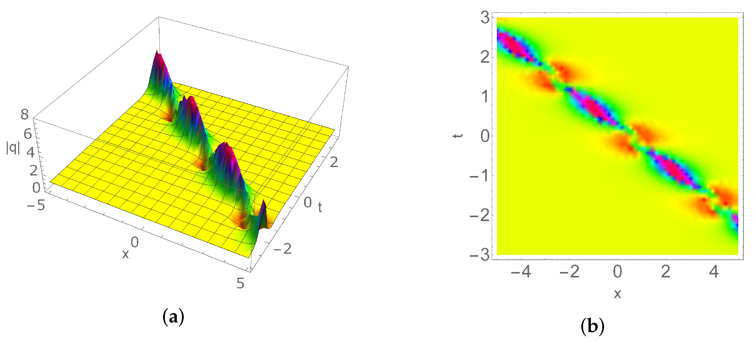
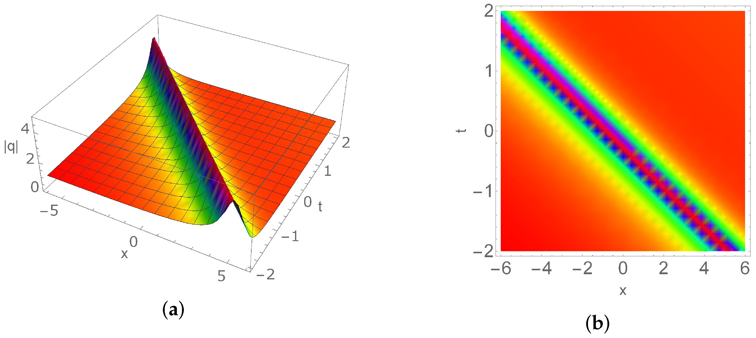
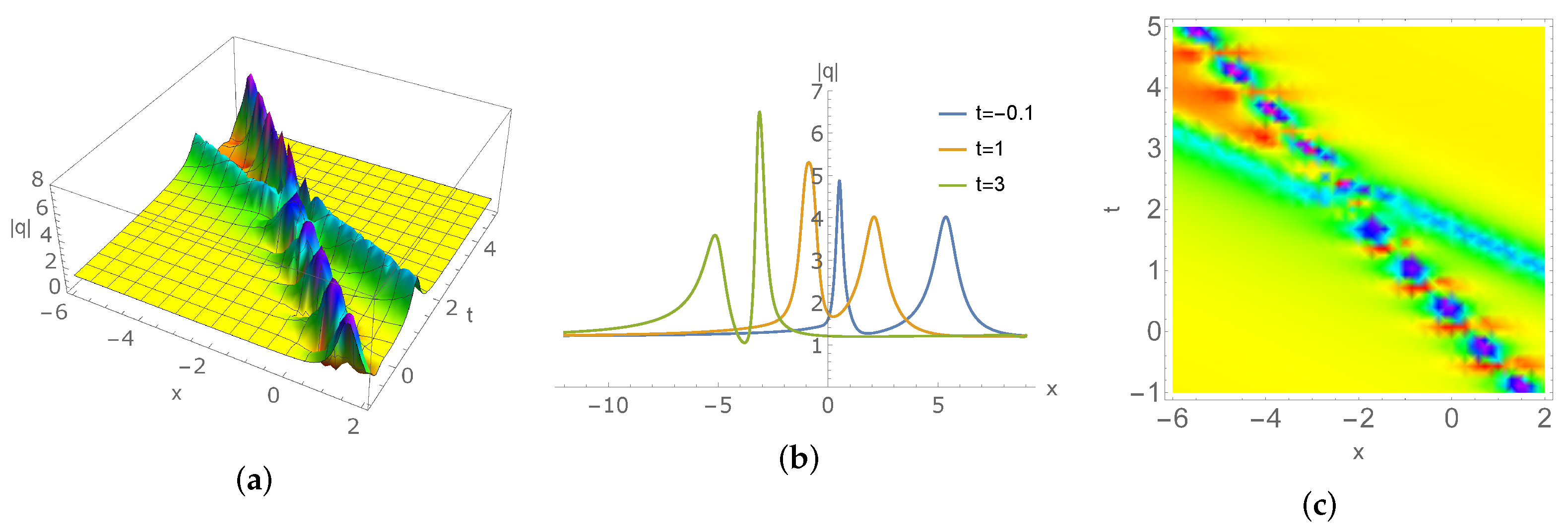
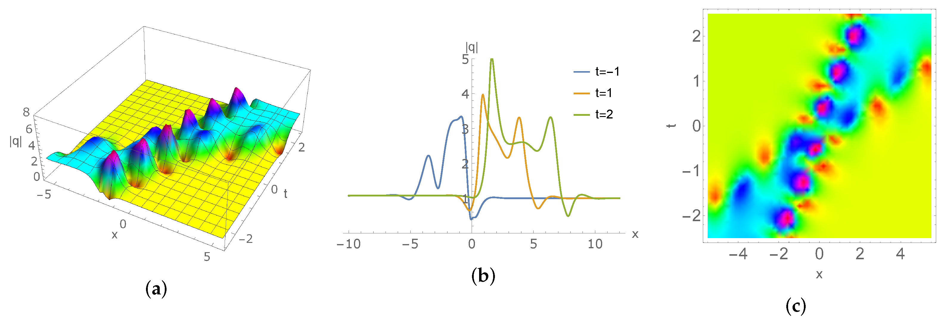
Figure 1. (a) One-breather of (50) with r = 0.5 , α = 0.8 , μ = 0.5 , ν = 0.5 , ϕ = 2 π , q 0 = 1 , (b) the corresponding density profile.
Mathematics 10 04424 g001
Figure 2. (a) One-soliton of (52) with β = 1.46 , κ = 1.35 , τ = 1.35 , ϕ = 2 π , q 0 = 1 , (b) the corresponding density profile.
Mathematics 10 04424 g002
Figure 3. (a,b) Interaction of the soliton and breather with r = 2.5 , α = 0.72 , β = 1.45 , μ = 0.45 , ν = 1.5 , κ = 0.5 , τ = 1.55 , ρ = 1 , q 0 = 1 , (c) the corresponding density profile.
Mathematics 10 04424 g003
Figure 4. (a,b) Interaction of the two breathers with r 1 = 0.42 , r 2 = 0.42 , α 1 = 0.25 , α 2 = 0.5 , μ = 0.2 , ν = 0.2 , κ = 0.5 , τ = 0.5 , ρ = 1 , q 0 = 1 , (c) the corresponding density profile.
Mathematics 10 04424 g004
Figure 5. (a,b) Interaction of the two solitons with β 1 = 0.5 , β 2 = 1 , μ = 1.2 , ν = 0.3 , κ = 1.2 , τ = 0.3 , ρ = 1 , q 0 = 1 , (c) the corresponding density profile.
Mathematics 10 04424 g005
Table 1. The relation between the type of soliton and the discrete spectrum N 1 and N 2 .
N 1 = 1 , N 2 = 0 N 1 = 0 , N 2 = 1 N 1 = 1 , N 2 = 1 N 1 = 2 , N 2 = 0 N 1 = 0 , N 2 = 2
one-breatherone-solitonsoliton-breathertwo-breathertwo-soliton
Publisher’s Note: MDPI stays neutral with regard to jurisdictional claims in published maps and institutional affiliations.

