Machine Learning for Music Genre Classification Using Visual Mel Spectrum

Abstract

Music is the most convenient and easy-to-use stress release tool in modern times. Many studies have shown that listening to appropriate music can release stress. However, since it is getting easier to make music, people only need to make it on the computer and upload it to streaming media such as Youtube, Spotify, or Beatport at any time, which makes it very infeasible to search a huge music database for music of a specific genre. In order to effectively search for specific types of music, we propose a novel method based on the visual Mel spectrum for music genre classification, and apply YOLOv4 as our neural network architecture. mAP was used as the scoring criterion of music genre classification in this study. After ten experiments, we obtained a highest mAP of 99.26%, and the average mAP was 97.93%.

1. Introduction

Social progress is very fast; people’s life pace is becoming more and more tense, resulting in a steady increase in suicide and crime rates. In order to reduce people’s life stress index from rising continuously, some methods need to be provided to release stress appropriately. Thence, quickly and effectively releasing stress has become an important topic for researchers.

Numerous studies have proven that stress can be relieved by listening to appropriate music [1,2,3]. However, the huge amount of music information makes the retrieval of appropriate music extremely difficult. In particular, the search process must efficiently and correctly classify music genres. Therefore, providing an effective music genre classification method will help towards appropriate music information retrieval. It has been shown in a lot of literature that music information retrieval has become one of the research fields that have received much attention in recent years. It mainly discusses various topics of music data retrieval, analyzes and organizes music data, and categorizes them according to composers, music forms, etc., to effectively provide demand for music. With the widespread use of the Internet and the advancement of audio compression coding, music is easily transmitted through the network. However, to obtain music, one must know the title or creator of the music, and this knowledge may be difficult to obtain for many people.

In 2003, Li et al. proposed a novel feature extraction method for music genre classification, DWCHs, which simultaneously captures local and global information of music signals by computing histograms of its Daubechies wavelet coefficients. They compared the effectiveness of this new feature with previously studied features using various machine learning classification algorithms, including support vector machines and linear discriminant analysis. The final results show that the use of DWCH significantly improves the accuracy of music genre classification [4]. In 2005, Li and Ogihara studied the application of taxonomy in the classification of music genres. Their experiments show that classification performance can be improved by using taxonomy. Furthermore, they also propose a method to automatically generate type classification based on a confusion matrix via linear discriminant projection [5]. In 2007, Meng et al. proposed a multivariate autoregressive feature model that provides two distinct feature sets—diagonal autoregressive (DAR) and multivariate autoregressive (MAR) features—to address the problem of music genre classification. They demonstrate the repeatability of the performance ranking of the temporal feature ensemble method by comparing with baseline mean variance and two other temporal feature ensemble techniques [6]. In 2018, Bahuleyan compared the performance of two classes of models with deep learning methods and traditional machine learning classifiers. His ensemble classifier combining the two proposed methods has an AUC value of 0.894 [7]. In 2020, Pelchat and Gelowitz reviewed some machine learning techniques used in music genre classification and also presented research work on music genre classification. They used spectrogram images generated from song time slices as input to the NN to classify songs into their respective musical genres [8].

In recent years, research on music genre classification by deep learning has sprung up. Liu et al. proposed a middle-level learning feature interaction method based on deep learning for the impact of learning feature interaction among different branches and layers on the final classification results in a multifeature model. Their experimental results show that their method has the best classification accuracy on the GTZAN dataset, reaching 93.65% [9]. Salazar proposed an MGC system by using two levels of hierarchical mining: GLCM (gray-level co-occurrence matrix) networks generated from the Mel spectrogram and a multihybrid feature strategy. They compared the RLS and accuracy values with several state-of-the-art methods and found that the accuracy obtained using micromining was more than 90% [10]. Singh and Biswas assessed and compared the robustness of some commonly used musical and nonmusical features on DL models for the MGC task by evaluating the performance of selected models on multiple employed features extracted from various datasets accounting for billions of segmented data samples. Their results showed that Mel-scale-based features and Swaragram have high robustness across the datasets over various DL models for the MGC task [11]. Shah et al. used support vector machines (SVM), random forests, XGB (eXtreme Gradient Boosting), and convolutional neural networks (CNN) to predict the genre of the audio signal. They proposed a comparison analysis for these models, and demonstrating that CNN outperforms machine learning models [12]. Lau and Ajoodha provided a comparative study on music genre classification using a deep learning convolutional neural network approach against five traditional off-the-shelf classifiers. They performed experiments on the popular GTZAN dataset and the results showed similar prediction results on test data at around 66% [13]. Kothari and Kumar demonstrated a music genre classification system based on neural networks. They described a complete processes for the music genre classification [14]. He divided it into multiple local musical instrument digital interface (MIDI) music passages, playing style close by analyzing passages, passage feature extracting, and the feature sequence of passages. He investigated recurrent neural networks (RNN) and attention using a distinctive sequence of input MIDI segments and collected 1920 MIDI files with genre labels from the Internet. Finally, he validated the method for it, combined with the experimental accuracy of equal-length segment categorization [15]. Qiu et al. proposed a musical instrument digital interface (MIDI) preprocessing method, Pitch to Vector (Pitch2vec), and a deep bidirectional transformer-based masked predictive encoder (MPE) method for music genre classification. They used the Lakh MIDI music dataset to evaluate the performance of their method, and their experimental results indicate that their method improves classification performance compared with state-of-the-art models [16]. Allamy and Koerich proposed a 1D residual convolutional neural network (CNN) architecture for music genre classification and compared it with other recent 1D CNN architectures. Their experimental results showed that this method achieves 80.93% of mean accuracy in classifying music genres and outperforms other 1D CNN architectures [17]. Prabhakar and Lee proposed five interesting and novel approaches, including a weighted visibility graph-based elastic net sparse classifier (WVG-ELNSC), a sequential machine learning analysis with stacked denoising autoencoder (SDA) classifier, Riemannian alliance-based tangent space mapping (RA-TSM) transfer learning techniques, a transfer support vector machine (TSVM) algorithm, and a deep learning classifier with bidirectional long short-term memory (BiLSTM)-cum-attention model with graphical convolution network (GCN), termed as a BAG deep learning model for music genre classification. Their experiments were performed on three music datasets: GTZAN, ISMIR 2004, and MagnaTagATune. They obtained a relatively higher classification accuracy of 93.51% when the deep learning BAG model was utilized [18].

In this study, in order to achieve a closer-to-the-human-ear perceptual pattern of audio, the Mel spectrum is used as the basis for visualizing the spectrum. The Mel spectrum was proposed by Davis and Mermelstein [19] in 1980. They argue that human auditory perception does not perceive the entire audio, but only focuses on certain areas. Through experiments, it has been found that the human auditory perception structure is like a filter that pays special attention to some specific frequency components. That is, it will only let sound at certain frequencies through and ignore other frequencies that are not of interest. Furthermore, the YOLOv4, which has not been used in music genre classification research, is used to train and validate visual spectrum, calculate mAP values, and achieve effective music genre classification.

2. Methods

2.1. Definition of Visual Mel Spectrum

The Mel spectrogram is mainly converted from audio through 5 steps. Step 1: Pre-emphasizing audio—this makes the sound sharp and crisp with reduced volume; Step 2: frame blocking—this makes each frame in the audio end-to-end, maintaining the continuity of the audio; Step 3: Adding window function—the main purpose is to enhance the function of audio framing and reduce the discontinuity of audio caused by sampling and quantization; Step 4: fast Fourier transform, which converts the audio from the time domain to the frequency domain; Step 5: mapping the FFT result onto the Mel scale, i.e., multiplying it by a set of 20 triangular bandpass filters. The above five steps can convert the audio into Mel spectrum. Visual Mel spectrum mainly converts the audio into the five-step Mel spectrum (that is, pre-emphasized audio, frame blocking, adding window function, fast Fourier transform, and mapping to the Mel scale), and before mapping to the Mel scale, with the horizontal axis as time and the vertical axis as frequency, plotting a spectrogram according to the audio power (dB) and then mapping it to the Mel scale. Therefore, the difference between visual Mel Spectrum and Mel spectrum is that Mel spectrum is a series of arrays or numbers, but the visual Mel spectrum is generated according to the power, so we can see the important characteristic distribution of the audio in the figure.

The following is the definition of visual Mel Spectrum.

Definition 1.

Visual Mel Spectrum is after pre-emphasizing audio, frame blocking, adding window function, and fast Fourier transform; the horizontal axis is time and the vertical axis is frequency; and the spectrum is plotted against audio power (dB) and then mapped to Mel Scale.

2.2. GTZAN Dataset

In this study, the GTZAN dataset (https://sites.google.com/site/yhcheng1981/downloads (accessed on 12 October 2022) is used as the dataset source for the experiments with a total capacity of 1.6 GB. The dataset was established by Tzanetakis and Cook [20], with a total of 1000 songs in 10 different genres, namely Blues, Classical, Country, Disco, Hiphop, Jazz, Metal, Pop, Reggae, and Rock; each genre contains 100 songs. In the GTZAN dataset, each song is 30 s long, with a 22,050 Hz sample rate, mono mode, AU file format, and 16-bit audio files. In this study, the dataset is divided into 70% as the training dataset, 20% as the test set, and 10% as the validation set.

Table 1. Contents of GTZAN dataset.

Item	Data
Genre	10
Length	30 s
Sample rate	22,050 Hz
Song mode	Mono
Song format	AU
Audio files	16 bits
Total	1000

shows the relevant information of the GTZAN dataset.

2.3. Data Preprocessing

Firstly, the visual spectrum diagram based on Mel spectrum is used as input. The original audio with 30 s is converted into Mel spectrum through MATLAB. We set the window function size to 1024 frames and overlap to 512 frames for maintaining the integrity of audio. Furthermore, we set the Fourier Transform size to 4096 frames and use 64 triangular bandpass filters for Mel scale filter. According to the horizontal axis time and vertical axis frequency, we draw the visual spectrum and use LabelImg to process the data, as shown in Figure 1. In Figure 1, the red box represents the feature area of the image in this area, and the corresponding red box coordinates are output xml file. We use deep learning to train the model by the xml files and the image files. The parameter settings are shown in

Table 2. Parameters of visual Mel spectrum.

Parameter	Value
Audio Length (seconds)	30
Window Length (frames)	1024
Overlap Length (frames)	512
FFT Length (frames)	4096
Num Bands (filters)	64

.

2.4. YOLOv4 for Music Genre Classification

2.4.1. Architecture

In this study, we use YOLOv4 [21] for music genre classification based on the visual Mel spectrum. YOLOv4 was proposed by Bochkovskiy et al. and is composed of five modules, including CBM, CBL, Res unit, CSPX, and SPP. CBM is the smallest module in the network structure and consists of Conv + Bn + Mish activation function. CBL is similar in structure to CBM; as shown in Figure 2, the difference is that CBL uses the Leaky ReLU activation function, while CBL uses Mish as the activation function. Res unit is based on the residual structure in Resnet, so a deeper network can be constructed, as shown in Figure 3. CSPX is a network structure based on SCPNet, which consists of three convolutional layers and X Res unit modules, as shown in Figure 4. SPP is to combine 1 × 1, 5 × 5, 9 × 9, 13 × 13 maximum pooling layers at multiple scales, and link features of different kernel sizes together as output, as shown in Figure 5.

2.4.2. Convolutional Neural Network

YOLOv4 is an algorithm based on convolutional neural network, and convolutional neural network is composed of convolutional layer, pooling layer, and fully connected layer. The convolution calculation consists of four parts: the input data size, the filter (Kernel map) size, stride, and the output data size, among which the filter and stride will directly affect the result of the convolution operation. Convolutional layer obtains the local features of the audio signal by sliding up and down a window with a customizable size in sequence, and then generates a feature map through the activation function as the input of the next layer, as shown in Figure 6. As can be seen in Figure 6, the blue box is the input, the red box is the 3 × 3 kernel map, and the purple box is the result, assuming that stride is set to 1 × 1; that is, the red box will be in the blue box according to 1 × 1 to moving, and if the number in the red box is the same as the number in the blue box, it is multiplied. When the first step is completed, the result in the purple box is 4, and other results can be obtained according to the same steps to obtain the complete result of the purple box.

The main function of the pooling layer is to compress the local features of the convolution, reduce the dimension of each feature map, and retain important features, so as to reduce computing resources and time. There are two common pooling layers: maximum pooling and average pooling. The method of maximum pooling is to reduce data by taking the maximum value, as shown in the upper part of Figure 7a, and the average pooling method is to reduce data by taking the average value, as shown in the lower half of Figure 7b. In YOLOv4, the maximum pooling method is used. The function of the full connection layer is to classify after receiving the characteristic information of the convolution layer and the pooling layer and obtain the classification result by adjusting the weight and deviation. Before entering the full connection layer, the dimension will be transformed through the flat layer, and then enter the full connection layer for classification.

In the backbone network in YOLOv4, the number of convolutional layers is the number of convolutional layers contained in each CSPX (CSPX = 3 + 2 × X convolutional layers), a total of 2 + (3 + 2 × 1) + 2 + (3 + 2 × 2) + 2 + (3 + 2 × 8) + 2 + (3 + 2 × 8) + 2 + (3 + 2 × 4) + 1, for a total of 72 convolutional layers. Bag of Freebies (BoF) and Bag of Specials (BoS) are used in YOLOv4 for object detection. During training, methods such as data augmentation, type imbalance, cost function, and soft labeling are often seen to improve accuracy. This improvement is called BoF because it does not affect inference speed, while BoS is a general term for actions that have less impact on inference speed but better performance, including CIoU-loss, CmBN, DropBlock regularization, Mosaic data enhancement, Self-Adversarial Training (SAT), Eliminate grid sensitivity, Cosine annealing scheduler, optimal hyperparameters, and random training shape. Among them, CIoU-loss is for the overlapping area of the correct answer box and the prediction box, minimizing the distance between the center points and maintaining the consistency of the height and width of the two boxes. Mosaic data enhancement method is to randomly select 4 pictures in the input picture set to randomly scale, randomly crop, randomly distort, and then stitch them together. CmBN is an improved method. Batch normalization uses the whitening layer as the input in the mini-batch to collect the average and variance of the sample, but when the data of the mini-batch is too small, a lot of noise will be generated. One solution is to estimate in multiple small batches of data, but the weights will collect statistical information with each iteration, which may cause the new weights to become inaccurate; that is to say, all of the average of the mini-batch is taken as wrong, and because the weight will change all the time, the cross-iteration batch normalization (CBN) therefore uses equations such as Equations (1)–(3) to adjust it based on k estimated data from previous iterations.

$${\overline{u}}_{t,k}^l\left({\theta }_t\right)=\frac{1}{k}{\displaystyle \sum }_{\tau =0}^{k-1}{u}_{t-\tau }^l\left({\theta }_t\right)$$

(1)

$${\overline{v}}_{t,k}^l\left({\theta }_t\right)=\frac{1}{k}{\displaystyle \sum }_{\tau =0}^{k-1}max\left[v_{t-\tau }^l\left({\theta }_t\right),u_{t-\tau }^l{\left({\theta }_t\right)}^2\right]$$

(2)

$${\overline{\sigma }}_{t,k}^l\left({\theta }_t\right)=\sqrt{{\overline{v}}_{t,k}^l\left({\theta }_t\right)-{\overline{u}}_{t,k}^l{\left({\theta }_t\right)}^2}$$

(3)

SAT is a data augmentation technique. In the traditional step, the weights of the model are adjusted during the backpropagation process to improve the ability of the detector, while in SAT, a forward direction is performed on the training samples. In propagation, SAT modifies the image so that it can reduce the performance of the detector at the maximum length, that is, an adversarial attack on the current model, which can improve the generalization ability of the model and reduce the occurrence of overfitting. Genetic algorithm is used in the optimal hyperparameter method, which finds the optimal solution of hyperparameters according to the concept of survival of the fittest. The random training shape improves the generalization of the one-stage object detector, which resizes the input image to different sizes instead of a fixed size. BoS includes Mish activation function, modified version of SPP module, modified version of SAM module, modified version of PAN path aggregation module, and DIoU-NMS. Among them, DIoU-NMS can make the model have a more stable response to the occlusion situation. Nonmaximum suppression (NMS) preserves bounding boxes with high confidence and filters out other bounding boxes that predict the same object. The DIoI method uses the distance between the IoI and the center point of the two bounding boxes when suppressing redundant bounding boxes.

2.4.3. Activation Function

In artificial neural network, the purpose of using activation function is to enhance the nonlinear change in neural network. A neural network without activation function is the same as matrix multiplication; even if a neural network with many layers is added, it is still matrix multiplication. The activation function is responsible for operating on the neuron and mapping the input of the neuron to the output. The activation function completes the learning of the model and makes it understand complex nonlinear functions. There are 6 kinds of activation functions commonly used in deep learning: sigmoid, tanh, ReLU, PReLU, Swish, and Mish. Sigmoid function is used to transfer the image with the value of (−∞, +∞) to (0, 1). Sigmoid has the advantages of stable optimization and easy operation. However, due to its soft saturation, it is easy to make the gradient disappear, resulting in training problems. The sigmoid function is shown in Equation (4).

$$\mathrm{g}\left(\mathrm{z}\right)=\frac{1}{1+{\mathrm{e}}^{-\mathrm{z}}}$$

(4)

The tanh function maps the number with the value of (−∞, +∞) to (−1, 1). tanh converges faster than sigmoid function, but it also has the disadvantage of the gradient disappearing due to saturation. The tanh function is shown in Equation (5).

$$\mathrm{g}\left(\mathrm{z}\right)=\frac{{\mathrm{e}}^{\mathrm{z}}-{\mathrm{e}}^{-\mathrm{z}}}{{\mathrm{e}}^{\mathrm{z}}+{\mathrm{e}}^{-\mathrm{z}}}$$

(5)

ReLU function, also known as rectified linear unit, is a piecewise linear function. ReLU can converge quickly in SGD, alleviate the problem of gradient disappearance, perform well in unsupervised pretraining, and provide sparse expression ability of neural network. However, with the progress of training, neuron death may occur, and the weight cannot be updated. As long as neuron death occurs, the gradient of neuron will always be 0 from this point, that is, irreversible death. The ReLU function is shown in Equation (6).

$$\mathrm{g}\left(\mathrm{z}\right)=\{\begin{array}{c}\mathrm{z},\mathrm{i}\mathrm{f}\mathrm{z}>0\\ 0,\mathrm{i}\mathrm{f}\mathrm{z}<0\end{array}$$

(6)

Leaky ReLU is a function that improves ReLU, also known as PReLU. Leaky ReLU solves the problem of neuron death of ReLU. It has a small positive slope in the negative region. Therefore, even for negative input values, it can carry out backpropagation with fast convergence speed and low error rate, but it cannot provide consistent relationship prediction for positive and negative input values. The results are inconsistent. Leaky ReLU function is shown in Equation (7).

$$\mathrm{g}\left(\mathrm{z}\right)=\{\begin{array}{c}\mathrm{z},\mathrm{i}\mathrm{f}\mathrm{z}>0\\ \mathrm{a}\mathrm{z},\mathrm{i}\mathrm{f}\mathrm{z}<0\end{array}$$

(7)

Swish is a smoothing function between linear function and ReLU function, so it is better than ReLU in deep model. Swish has no upper boundary, so there will be no gradient saturation. At the same time, it has lower boundary, which can produce stronger regularization effect. Swish training is easy but unstable, and there will be different results in different tasks. The Swish function is shown in Equation (8).

$$\mathrm{f}\left(\mathrm{x}\right)={\mathrm{x}}^{*}\frac{1}{1+{\mathrm{e}}^{-\mathrm{z}}}$$

(8)

Mish is a self-regularized nonmonotonic neural activation function. Mish has the characteristics of low cost, smooth curve, and being nonmonotone, upper-unbounded and lower-bounded, but the amount of calculation is large. No upper bound is the characteristic required by any activation function, because it avoids the gradient saturation that leads to the sharp decline in training speed. The nonmonotonic function helps to maintain a small negative value, so as to stabilize the network gradient. Mish is a smooth function, which has good generalization ability and effective optimization ability of results, and can improve the quality of results. The Mish function is shown in Equation (9).

$$\mathrm{f}\left(\mathrm{x}\right)=\mathrm{x}\ast \tanh \left(\ln \left(1+{\mathrm{e}}^{\mathrm{x}}\right)\right)$$

(9)

Compared with ReLU, Mish only takes one second more in each epoch, and the result is better than ReLU, and using ReLU as the activation function may cause the gradient to explode, and the output has no upper limit, so backbone in YOLOv4 is most suitable to use Mish as the activation function, while the latter network uses Leaky ReLU as the activation function.

Table 3. Comparison the functions of Mish, Swish, and ReLU [22].

Model	Mish	Swish	ReLU
Resnet v2-20	92.02%	91.61%	91.71%
WRN 10-2	86.83%	86.56%	84.56%
Simple Net	91.70%	91.44%	91.16%
Xception Net	88.73%	88.56%	88.38%
Capsule Net	83.15%	82.48%	82.19%
Inception ResNet v2	85.21%	84.96%	82.22%

Bold shows the highest value.

shows the comparison between the Mish activation function and the Swish and ReLU activation functions [22]. The data in Table 3 are obtained according to Top-1 accuracy on CIFAR-10 dataset that can be referred to [22]. The CIFAR-10 dataset consists of 60,000 32 × 32 color images in 10 classes, with 6000 images per class. There are 50,000 training images and 10,000 test images. From Table 3, we can find that the Mish activation function has good results in various model architectures compared with other activation functions. Because the Mish activation function has been tested on such a large number of training images, it is reliably used in image-based models. The reason for Mish as the activation function of the first layer.

2.4.4. Dropblock

Dropblock is used to replace Dropout. The traditional Dropout is shown on the left side of Figure 8. It can be seen that Dropout will randomly prevent neurons from participating in this iterative training to prevent overfitting. Overfitting means that the neural network learns the features too thoroughly, whether they are correct or wrong data, which contains noise and which leads to the high learning accuracy of the neural network, but the generalization and identification accuracy are very low. Because the convolution layer is not sensitive to the way of random discarding, this is because the convolution layer is usually used at the same time with the pooled and fully connected layers. Even if the convolution layer is discarded randomly, the convolution layer can still learn the same information from the adjacent activation units, and the benefit is not high. Therefore, Dropblock is used in YOLOv4, which will be discarded together with adjacent neurons according to the discarded neurons, as shown on the right side of Figure 8.

3. Results and Discussion

3.1. Evaluation Criteria

In this research, the audio files in GTZAN are converted into a visualized Mel spectrum and then the experiment is carried out according to the training, verification and testing ratio. Precision, Recall, F1-score, mAP and confusion matrix are used to analyze the experimental results, the main scoring basis is mAP, and Equation (10) is the calculation method of mAP. Among them, classes is the number of categories. This experiment uses 10 music genres, so the number of categories is 10. TP(c) is the actual prediction for category c, and FP(c) is the prediction for category c. Equation (11) is the formula of the Precision algorithm, in which TP is the actual prediction, and FP is the prediction. The purpose of calculating Precision is to calculate the proportion of TP, that is, the proportion that is predicted to be true and actually correct in the prediction. Equation (12) is the formula of the Recall algorithm, where FN is the prediction that there is no actual absence, and the purpose of calculating the Recall is to calculate the proportion of positive samples that are correctly identified as positive. Equation (13) is the formula of the F1-score, and the F1-score is the harmonic mean of Precision and Recall, which is an indicator used to measure the accuracy of the two-class model. Equation (14) is the formula of the accuracy scoring index. The accuracy scoring method is applicable to the two-classification model, and the GTZAN dataset used in this study has 10 classes, which belong to multiclassification. Therefore, using accuracy as the scoring index cannot accurately display the accuracy of the model. The purpose of providing accuracy is to compare with the traditional music genre classification method. It can be seen from Equation (14) that accuracy only evaluates TP and TN when scoring, which makes this scoring method able to be used as an excellent scoring index in the balanced data. However, due to the use of random sampling when splitting the training set, verification set and test set, the proportion of each song genre in the test set is unbalanced, and the proportion of each song genre can be seen from the confusion matrix.

$$mAP=\frac{1}{\left|classes\right|}\ast {\displaystyle \sum }_{c\in class\mathrm{e}s}\frac{TP\left(c\right)}{TP\left(c\right)+FP\left(c\right)}$$

(10)

$$precision=\frac{TP}{TP+FP}$$

(11)

$$RecaII=\frac{TP}{TP+FN}$$

(12)

$$F1-score=\frac{2\ast \left(R\mathrm{e}call\ast Pr\mathrm{e}cision\right)}{Recall+Precision}$$

(13)

$$Accuracy=\frac{TP+TN}{TP+TN+FP+FN}$$

(14)

3.2. Parameter Settings for Deep Learning Experiments

The parameters of this study are to set epochs to 20,000 times, the batch size to 64, the subdivisions to 16, and the input size length and width to 416 × 416. In order to prevent the influences of randomizing training and to increase the average accuracy of the experiments, this study conducted 10 experiments and calculated the average value to obtain more correct and stable accuracy.

3.3. Results and Analysis

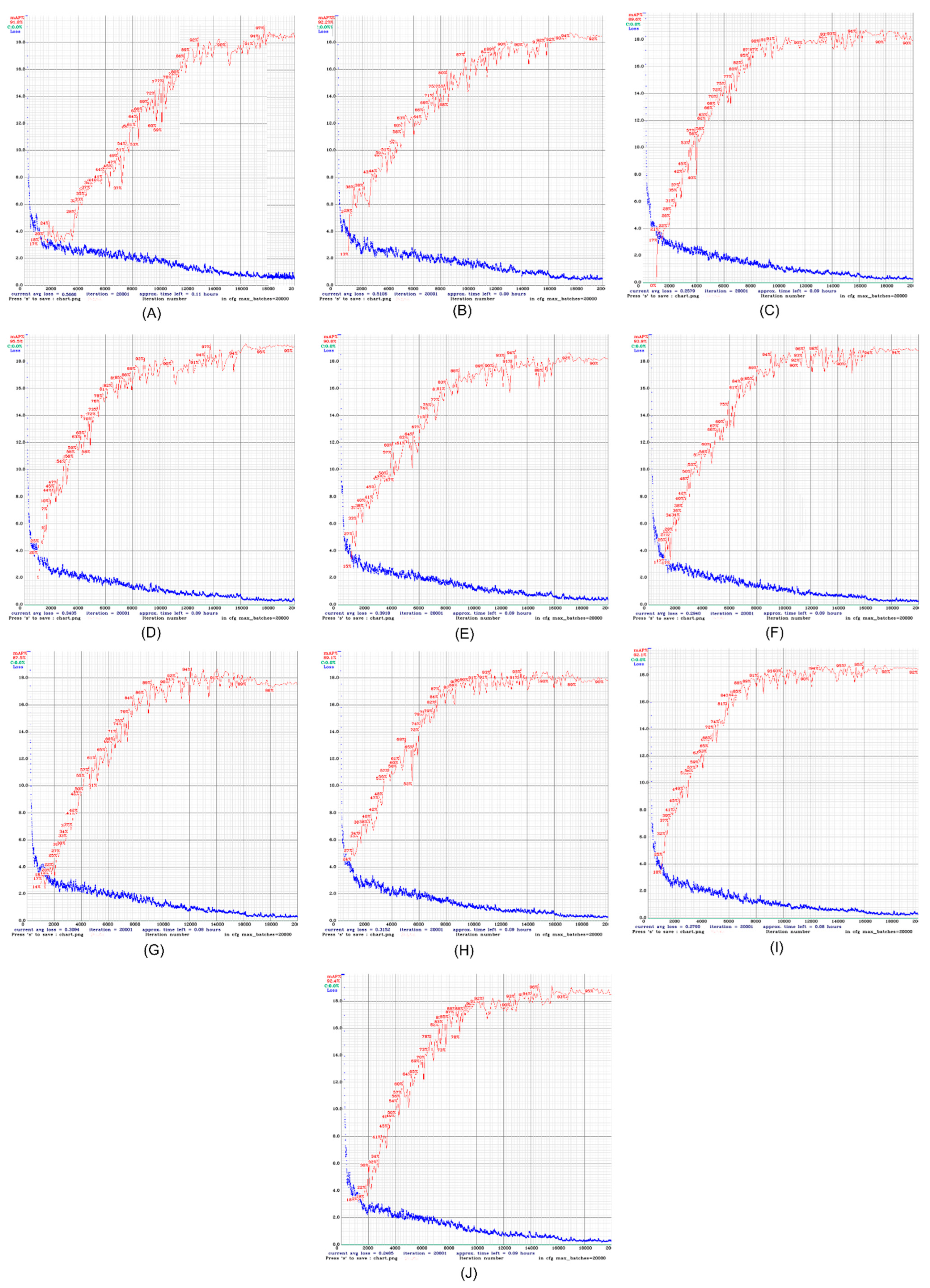
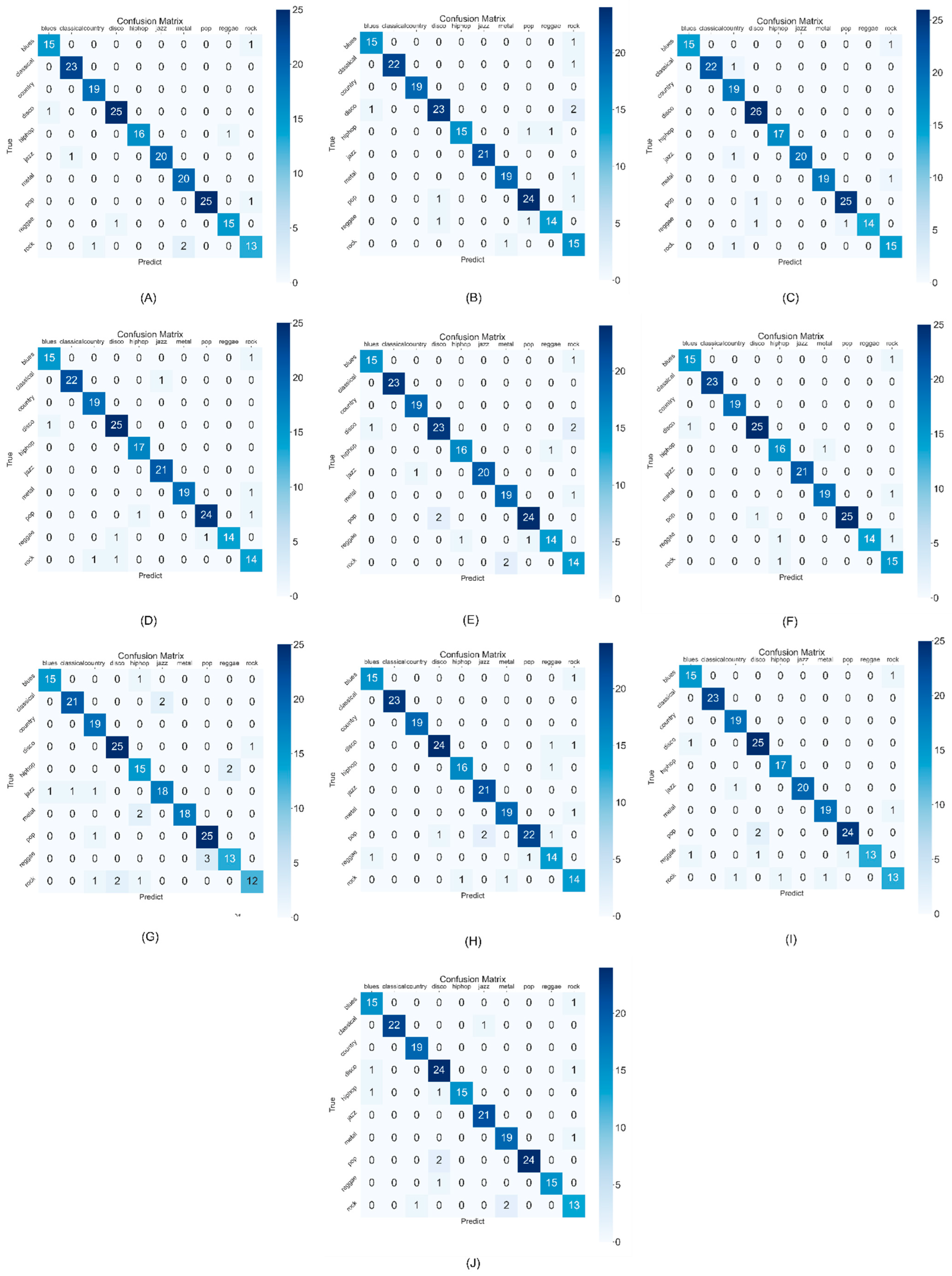
Figure 9A shows the mAP curve and average loss curve of the first experimental results. The results show that when the epoch number is set to 20,000, the mAP value reaches 91.8%, and the average loss rate is 0.5666. Figure 10A shows the confusion matrix using the weights of the first experiment on the test set. The results show a mAP result of 94.57% using the test set, Precision of 0.96, Recall of 0.96, F1-score of 0.96, and Accuracy of 0.955. 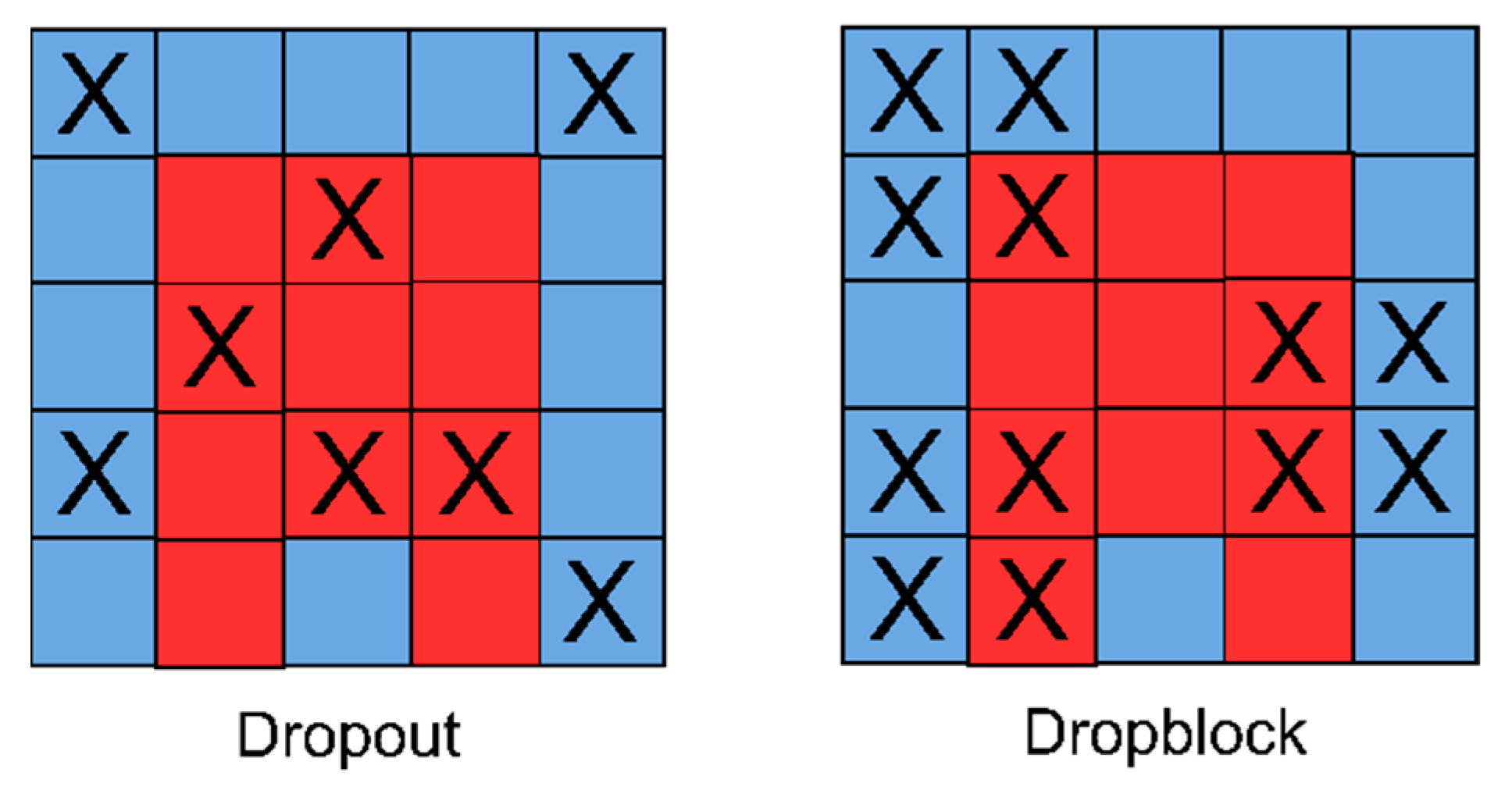From Figure 9A, the mAP value increased in a curve from 17% at the beginning to 97% at the highest value, while the average figure was 91.8%. It can be seen that the curve rises and occasionally falls, but continues to rise upwards. Therefore, the results show that the Dropblock of the model plays a role in learning, so that the machine reduces the incidence of overfitting during the learning process. Trends falling and rising indicate that the model is learning steadily rather than one-shot, which also indicates that the generalization ability of the model will be improved. As can be seen from Figure 10, there are a total of 200 songs in the test set for testing. These songs are not applied to the training process, so they can be used as data to judge the quality of the model. It can be seen that the song distribution of 10 genres is not balanced, adding the number of songs on the x-axis is the total number of genres in the test set, such as 16 blues, 23 classical, and so on. The number of songs of each genre in the test set is shown in

Table 4. Number of songs in 10 genres.

Genre	Number of Songs
Blues	16
Classical	23
Country	19
Disco	26
Hip-hop	17
Jazz	21
Metal	20
Pop	26
Reggae	16
Rock	16
Total	200

. Therefore, as mentioned above, our method is not accurate in the accuracy scoring index. In the confusion matrix, the x-axis is the order in which the model predicts the music styles, and the y-axis is the order in which the real music styles are. Therefore, the result of cross comparison is that the middle color is darker, that is, the model predicts the correct number of songs in the test set. From this result, it can be seen that our method can obtain good accuracy in the test set, but there are still some genre classification errors. The reason will be analyzed in the last of the results.

Figure 9B shows the mAP curve and the average loss curve of the second experimental results, where the mAP value is 92.2%, the average loss rate is 0.5106, and the number of epochs is 20,000. Figure 10B shows the confusion matrix using the second experiment weights on the test set, and the Precision is 0.95, the Recall is 0.97, the F1-score is 0.96, the Accuracy is 0.935, and the mAP result using the test set is 96.48%. As can be seen from Figure 9B, compared with the first experiment, the increase rate of mAP in the second experiment is faster and continues to rise. Therefore, compared with 91.8% in the first experiment, the accuracy of the second experiment reaches 92.2%, and the map curve tends to be stable when the epochs are 16,000, while it has been stable since the epochs is 14,000 in the first experiment, resulting in better results in the second experiment.

Figure 9C shows the mAP curve and the average loss curve of the third experimental results, where the mAP value is 89.6%, the average loss rate is 0.2579, and the number of epochs is 20,000. Figure 10C shows the confusion matrix using the third experiment weights on the test set, and the Precision is 0.95, the Recall is 0.96, the F1-score is 0.96, the Accuracy is 0.96, and the mAP result using the test set is 97.84%. As can be seen from Figure 9C, compared with the second experiment, the front part of the mAP curve in the third experiment rises steeply, and there are large fluctuations in the later stage. Therefore, the average mAP value is 89.6%, which is lower than 92.2% in the second experiment, which means that if you learn everything too fast and the epoch times are not prolonged, the training accuracy will be low. The average loss curve also shows a gradual decline and tends to be stable. Compared with the average loss curve of the second experiment, the fluctuation of the average loss curve of the third experiment is smaller than that of the second experiment. Therefore, the average loss rate comes to 0.2579, half of that of the second experiment.

Figure 9D shows the mAP curve and the average loss curve of the fourth experimental results, where the mAP value is 95.5%, the average loss rate is 0.3435, and the number of epochs is 20,000. Figure 10D shows the confusion matrix using the fourth experiment weights on the test set, and the Precision is 0.94, the Recall is 0.99, the F1-score is 0.97, the Accuracy is 0.95, and the mAP result using the test set is 98.82%. As can be seen from Figure 9D, the mAP curve of the fourth experiment has a larger amplitude than that of the previous two experiments, so there is a higher mAP value when the epochs are 16,000. The average loss curve also shows a continuous downward and stable trend, reaching the value of 0.3435, which is similar to the third experiment. The fluctuation range of the curve is also small, but it is larger than the value of the third experiment.

Figure 9E shows the mAP curve and the average loss curve of the fifth experimental results, where the mAP value is 90.8%, the average loss rate is 0.3918, and the number of epochs is 20,000. Figure 10E shows the confusion matrix using the fifth experiment weights on the test set, and the Precision is 0.94, the Recall is 0.96, the F1-score is 0.95, the Accuracy is 0.935, and the mAP result using the test set is 98.81%. As can be seen from Figure 9E, the mAP curve of the fifth experiment is relatively unstable compared with the first three experiments, and the curve rise is not high when the epochs are 4000 to 6000, and the first four experiments have fluctuations. But the duration is less, and the duration of the fifth experiment is about 2000 epochs, which may be the reason why the average mAP of the fifth experiment is only 90.8%.

Figure 9F shows the mAP curve and the average loss curve of the sixth experimental results, where the mAP value is 93.9%, the average loss rate is 0.2940, and the number of epochs is 20,000. Figure 10F shows the confusion matrix using the sixth experiment weights on the test set, and the Precision is 0.93, the Recall is 0.96, the F1-score is 0.95, the Accuracy is 0.96, and the mAP result using the test set is 98.53%. As can be seen from Figure 9F, the sixth experiment obtained the maximum mAP value of 96%, and there was a large curve fluctuation between epochs 12,000 and epochs 15,000, but since the mAP value at that time had reached a high point, the average value is accurate. The accuracy rate has little effect. It can be concluded that the average accuracy rate is 93.9%, and the average loss rate is also reduced to 0.2940, which is close to the average loss rate of the third experiment.

Figure 9G shows the mAP curve and the average loss curve of the seventh experimental results, where the mAP value is 87.5%, the average loss rate is 0.3094, and the number of epochs is 20,000. Figure 10G shows the confusion matrix using the sixth experiment weights on the test set, and the Precision is 0.87, the Recall is 0.96, the F1-score is 0.91, the Accuracy is 0.905, and the mAP result using the test set is 99.26%. It can be seen from Figure 9G that in the seventh experiment, the curve slipped when the epochs were 16,000, and the AP fluctuated greatly at each epoch, which resulted in the mAP value of this experiment being only 87.5%. Although the average loss curve also showed a continuous downward trend, it finally stayed at 0.3094.

Figure 9H shows the mAP curve and the average loss curve of the eighth experimental results, where the mAP value is 89.1%, the average loss rate is 0.3152, and the number of epochs is 20,000. Figure 10H shows the confusion matrix using the eighth experiment weights on the test set, and the Precision is 0.91, the Recall is 0.94, the F1-score is 0.93, the Accuracy is 0.935, and the mAP result using the test set is 97.91%. It can be seen from Figure 9H that in the eighth experiment, the curve also showed a downward trend after the epochs were 18,000, but the magnitude was not as large as that in the seventh experiment, so the mAP value was not so much affected, reaching 89.1%. The average loss rate fluctuates greatly when the epochs are 2000 to 4000, and then stabilizes in the later period, but there is still room for decline in terms of trends.

Figure 9I shows the mAP curve and the average loss curve of the ninth experimental results, where the mAP value is 92.1%, the average loss rate is 0.2790, and the number of epochs is 20,000. Figure 10I shows the confusion matrix using the ninth experiment weights on the test set, and the Precision is 0.96, the Recall is 0.98, the F1-score is 0.97, the Accuracy is 0.94, and the mAP result using the test set is 98.87%. It can be seen from Figure 9I that the mAP curve of the ninth experiment is similar to that of the fourth experiment; the difference is that the time for the fourth experiment to stabilize is later than that of the ninth experiment, so a higher accuracy rate is obtained. Compared with the fourth experiment, the average loss rate of the ninth experiment was lower than that of the fourth experiment, reaching a value of 0.2790.

Figure 9J shows the mAP curve and the average loss curve of the ninth experimental results, where the mAP value is 92.4%, the average loss rate is 0.2485, and the number of Epochs is 20,000. Figure 10J shows the confusion matrix using the ninth experiment weights on the test set, and the Precision is 0.95, the Recall is 0.95, the F1-score is 0.95, the Accuracy is 0.935, and the mAP result using the test set is 98.19%. It can be seen from Figure 9J that the results of the tenth experiment are close to the results of the second experiment, but the difference from the second experiment is that the mAP value of the tenth experiment is steeper when rising. The average loss rate was half that of the second experiment, coming to 0.2485.

3.4. Test for the Number of Training Sessions

To test whether the proposed method and parameters are limited by the number of training sessions, the same dataset, same server, and the same parameters and settings were used and the number of epochs was increased to 40,000. Figure 11 shows the mAP curve and the mean loss curve with epochs set to 40,000 times. As can be seen from Figure 11, the mAP value of the experimental results is 81.2%, and the average loss rate is 0.0803. Furthermore, the mAP value stabilizes when the epochs are at 20,000 times. Therefore, when the epochs increased to 40,000 times, the accuracy did not improve and the average loss rate was close to zero. This result shows that the results of the proposed method have reached the best value.

Table 5. Results of 10 experiments.

Number of Experiments	mAP of Training	mAP of Testing
1	91.8%	94.57%
2	92.2%	96.48%
3	89.6%	97.84%
4	95.5%	98.82%
5	90.8%	98.81%
6	93.9%	98.53%
7	87.5%	99.26%
8	89.1%	97.91%
9	92.1%	98.87%
10	92.4%	98.19%

shows the individual mAP values for 10 experiments. The results of these 10 experiments yielded an average mAP value of 91.49%.

3.5. Comparison of the AVG Accuracy of the Proposed Method with Other Methods

In order to demonstrate that the proposed method is feasible, we compare the results of the proposed method with five other methods in the literature. The other methods do not provide indicators such as average mAP, average precision, average recall, and average F1-score; therefore, only the AVG accuracy is compared in this study. The results are shown in

Table 6. Comparison of the proposed method with other methods in AVG accuracy.

Methods	AVG Accuracy
Our method	94.5%
Elbir et al.’s method (Data from [23])	72.6%
Rajan and Murthy’s method (Data from [24])	75.5%
Kobayashi et al.s’ method (Data from [25])	81.5%
Zheng et al.’s method (Data from [26])	84.7%
Benetos and Kotropoulos’s method (Data from [27])	78.9%

. From these results, we found that our method obtained an extremely high 94.5% AVG accuracy and is superior to the five other methods in the literature.

4. Conclusions

The results of our experiment show the feasibility of the graphical spectrum. From the results of the 10 experiments, it can be seen that the map value of the 10 experiments is more than 80% or even 95.5%, and the overall trend of the map curve of each experiment increases upward, which shows the feasibility of using the visual Mel spectrum to the GTZAN dataset. In this study, the original audios were converted into their respective visual Mel spectrum, and a total of 10 experiments were performed with a ratio of 70% training set, 20% testing set, and 10% validation set. The average mAP of the training results is 91.49%, and the average mAP of the test set is 97.93%. In conclusion, this study introduces the innovative visual Mel spectrum for music genre classification. The experimental results show that the method proposed can indeed effectively promote music genre classification. The advantage of using a graphical spectrum diagram is that it has high generalization and does not require the building of a professional audio model. The disadvantage is that a high hardware cost needs to be spent. Future works are suggested for the researchers as follows:

(1)

Collect representative datasets to verify the accuracy and generalization of this research method.

(2)

Integrate several representative datasets to develop a complete visual Mel spectrum dataset for music genre classification.

(3)

Investigate other novel deep learning methods to explore the benefits of using the visual Mel spectrum dataset.

(4)

Discuss and introduce improvement strategies in music genre classification to promote better performance and results in music classification results.

(5)

Develop friendly and available systems for the convenience of music genre classification.

Finally, the significance and innovation of this study are summarized as follows:

(1)

This study proposes the novel visual Mel spectrum, which is different from the traditional Mel spectrum for music genre classification, and is an innovative study.

(2)

YOLO has never been used to music genre classification. This study is the first to use YOLO for music genre classification and has research value.

(3)

The visual Mel spectrum combined with YOLO achieves higher accuracy compared with other methods, which is a forward-looking method.

References

1. Hillecke, T.; Nickel, A.; Bolay, H.V. Scientific perspectives on music therapy. Ann. N. Y. Acad. Sci. 2005, 1060, 271–282. [Google Scholar] [CrossRef]
2. Yehuda, N. Music and stress. J. Adult Dev. 2011, 18, 85–94. [Google Scholar] [CrossRef]
3. Thoma, M.V.; La Marca, R.; Brönnimann, R.; Finkel, L.; Ehlert, U.; Nater, U.M. The effect of music on the human stress response. PLoS ONE 2013, 8, e70156. [Google Scholar] [CrossRef] [Green Version]
4. Li, T.; Ogihara, M.; Li, Q. A comparative study on content-based music genre classification. In Proceedings of the 26th Annual International ACM SIGIR Conference on Research and Development in Informaion Retrieval, Toronto, ON, Canada, 28 July–1 August 2003; pp. 282–289. [Google Scholar]
5. Li, T.; Ogihara, M. Music genre classification with taxonomy. In Proceedings of the IEEE International Conference on Acoustics, Speech, and Signal Processing (ICASSP’05), Philadelphia, PA, USA, 18–23 March 2005; Volume 195, pp. v/197–v/200. [Google Scholar]
6. Meng, A.; Ahrendt, P.; Larsen, J.; Hansen, L.K. Temporal feature integration for music genre classification. IEEE Trans. Audio Speech Lang. Process. 2007, 15, 1654–1664. [Google Scholar] [CrossRef] [Green Version]
7. Bahuleyan, H. Music genre classification using machine learning techniques. arXiv 2018, arXiv:1804.01149. [Google Scholar]
8. Pelchat, N.; Gelowitz, C.M. Neural network music genre classification. Can. J. Electr. Comput. Eng. 2020, 43, 170–173. [Google Scholar] [CrossRef]
9. Liu, J.; Wang, C.; Zha, L. A Middle-Level Learning Feature Interaction Method with Deep Learning for Multi-Feature Music Genre Classification. Electronics 2021, 10, 2206. [Google Scholar] [CrossRef]
10. Salazar, A.E.C. Hierarchical mining with complex networks for music genre classification. Digit. Signal Process. 2022, 127, 103559. [Google Scholar] [CrossRef]
11. Singh, Y.; Biswas, A. Robustness of musical features on deep learning models for music genre classification. Expert Syst. Appl. 2022, 199, 116879. [Google Scholar] [CrossRef]
12. Shah, M.; Pujara, N.; Mangaroliya, K.; Gohil, L.; Vyas, T.; Degadwala, S. Music Genre Classification using Deep Learning. In Proceedings of the 2022 6th International Conference on Computing Methodologies and Communication (ICCMC), Erode, India, 29–31 March 2022; pp. 974–978. [Google Scholar]
13. Lau, D.S.; Ajoodha, R. Music Genre Classification: A Comparative Study between Deep Learning and Traditional Machine Learning Approaches. In Proceedings of the Sixth International Congress on Information and Communication Technology, London, UK, 25–26 February 2021; pp. 239–247. [Google Scholar]
14. Kothari, N.; Kumar, P. Literature Survey for Music Genre Classification Using Neural Network. Int. Res. J. Eng. Technol. 2022, 9, 691–695. [Google Scholar]
15. He, Q. A Music Genre Classification Method Based on Deep Learning. Math. Probl. Eng. 2022, 2022, 9668018. [Google Scholar] [CrossRef]
16. Qiu, L.; Li, S.; Sung, Y. DBTMPE: Deep bidirectional transformers-based masked predictive encoder approach for music genre classification. Mathematics 2021, 9, 530. [Google Scholar] [CrossRef]
17. Allamy, S.; Koerich, A.L. 1D CNN architectures for music genre classification. In Proceedings of the 2021 IEEE Symposium Series on Computational Intelligence (SSCI), Virtual, 5–7 December 2021; pp. 1–7. [Google Scholar]
18. Prabhakar, S.K.; Lee, S.-W. Holistic Approaches to Music Genre Classification using Efficient Transfer and Deep Learning Techniques. Expert Syst. Appl. 2023, 211, 118636. [Google Scholar] [CrossRef]
19. Davis, S.; Mermelstein, P. Comparison of parametric representations for monosyllabic word recognition in continuously spoken sentences. IEEE Trans. Acoust. Speech Signal Process. 1980, 28, 357–366. [Google Scholar] [CrossRef] [Green Version]
20. Tzanetakis, G.; Cook, P. Musical genre classification of audio signals. IEEE Trans. Speech Audio Process. 2002, 10, 293–302. [Google Scholar] [CrossRef]
21. Bochkovskiy, A.; Wang, C.-Y.; Liao, H.-Y.M. Yolov4: Optimal speed and accuracy of object detection. arXiv 2020, arXiv:2004.10934. [Google Scholar]
22. Misra, D. Mish: A self regularized non-monotonic neural activation function. arXiv 2019, arXiv:1908.08681. [Google Scholar]
23. Elbir, A.; Çam, H.B.; Iyican, M.E.; Öztürk, B.; Aydin, N. Music genre classification and recommendation by using machine learning techniques. In Proceedings of the 2018 Innovations in Intelligent Systems and Applications Conference (ASYU), Adana, Turkey, 4–6 October 2018; pp. 1–5. [Google Scholar]
24. Rajan, R.; Murthy, H.A. Music genre classification by fusion of modified group delay and melodic features. In Proceedings of the 2017 Twenty-Third National Conference on Communications (NCC), Chennai, India, 2–4 March 2017; pp. 1–6. [Google Scholar]
25. Kobayashi, T.; Kubota, A.; Suzuki, Y. Audio feature extraction based on sub-band signal correlations for music genre classification. In Proceedings of the 2018 IEEE International Symposium on Multimedia (ISM), Taichung, Taiwan, 10–12 December 2018; pp. 180–181. [Google Scholar]
26. Zheng, E.; Moh, M.; Moh, T.-S. Music genre classification: A n-gram based musicological approach. In Proceedings of the 2017 IEEE 7th International Advance Computing Conference (IACC), Hyderabad, India, 5–7 January 2017; pp. 671–677. [Google Scholar]
27. Benetos, E.; Kotropoulos, C. Non-negative tensor factorization applied to music genre classification. IEEE Trans. Audio Speech Lang. Process. 2010, 18, 1955–1967. [Google Scholar] [CrossRef]
Figure 1. Construction of visual Mel spectrum.
Mathematics 10 04427 g001
Figure 2. CBL and CBM modules.
Mathematics 10 04427 g002
Figure 3. Res unit module.
Mathematics 10 04427 g003
Figure 4. CSPX unit module.
Mathematics 10 04427 g004
Figure 5. SPP unit module.
Mathematics 10 04427 g005
Figure 6. Convolution calculation.
Mathematics 10 04427 g006
Figure 7. Pooling layer. (a) the maximum pooling; (b) the average pooling.
Mathematics 10 04427 g007
Figure 8. Schematic of Dropout and Dropblock.
Mathematics 10 04427 g008
Figure 9. mAP and loss curves of the experimental training.
Mathematics 10 04427 g009
Figure 10. Confusion matrix of the experiments.
Mathematics 10 04427 g010
Figure 11. Experimental results of 40,000 epochs.
Mathematics 10 04427 g011