Article

Deep Learning-Based Cyber–Physical Feature Fusion for Anomaly Detection in Industrial Control Systems

1
Department of Network Engineering, Chengdu University of Information Technology, Chengdu 610225, China
2
Department of Informatics and Networked Systems, University of Pittsburgh, Pittsburgh, PA 15260, USA
*
Author to whom correspondence should be addressed.
Mathematics 2022, 10(22), 4373; https://doi.org/10.3390/math10224373
Submission received: 23 October 2022 / Revised: 15 November 2022 / Accepted: 18 November 2022 / Published: 20 November 2022

Abstract

:
In this paper, we propose an unsupervised anomaly detection method based on the Autoencoder with Long Short-Term Memory (LSTM-Autoencoder) network and Generative Adversarial Network (GAN) to detect anomalies in industrial control system (ICS) using cyber–physical fusion features. This method improves the recall of anomaly detection and overcomes the challenges of unbalanced datasets and insufficient labeled samples in ICS. As a first step, additional network features are extracted and fused with physical features to create a cyber–physical dataset. Following this, the model is trained using normal data to ensure that it can properly reconstruct the normal data. In the testing phase, samples with unknown labels are used as inputs to the model. The model will output an anomaly score for each sample, and whether a sample is anomalous depends on whether the anomaly score exceeds the threshold. Whether using supervised or unsupervised algorithms, experimentation has shown that (1) cyber–physical fusion features can significantly improve the performance of anomaly detection algorithms; (2) the proposed method outperforms several other unsupervised anomaly detection methods in terms of accuracy, recall, and F1 score; (3) the proposed method can detect the majority of anomalous events with a low false negative rate.

1. Introduction

In recent years, cyberattacks have caused significant damage to industrial production and national infrastructure [1]; the Stuxnet virus swept the global industry in 2010 and was able to carry out targeted attacks on infrastructure, with Iran suffering the most severe effects [2]. In 2015, a malicious program called BlackEnergy affected multiple substations in the Ukrainian power sector [3]. Many Ukrainian government agencies and companies were attacked by the ransomware NotPetya in 2017, which ultimately caused havoc worldwide [4]. A serious disaster can also result from the failure of hardware or software within an ICS as well as threats from the Internet. Globally, ICS security incidents occur frequently.
In order to secure ICS, anomaly detection is a promising approach [5]. It is usually physical faults or network attacks that cause anomalous events to occur in ICS. Sensors, actuators, pipelines, and other industrial equipment may malfunction due to physical faults. A network attack refers to an attack on a communication channel, host, or process control system, such as a man-in-the-middle attack (MITM), a denial of service (DoS), or a scanning attack. The purpose of industrial sensors is to collect status information (referred to in this paper as physical information) about the various industrial equipment in the system and to reflect the physical processes that take place within it. Physical faults have an impact on the physical operation of the system, but not on its network traffic. This results in physical faults not being detected by anomaly detection methods based solely on network traffic. The physical processes of a system may not necessarily be affected by some network attacks. Consequently, algorithms that detect anomalies based solely on physical information are not able to detect these attacks. The use of anomaly detection algorithms that are based solely on physical information cannot detect network attacks in a timely manner, since most network attacks against ICS do not immediately cause the system to enter an abnormal state. Our conclusion is that taking into account both network traffic information and physical information is an effective way to improve the detection performance for anomaly detection algorithms that are used in industrial control systems [6], which has tended to be ignored in past studies.
In the past decade, artificial intelligence (AI) has been rapidly developed and applied in various fields [7,8,9,10]. A number of AI-based approaches have emerged in ICS security, which can be categorized as supervised and unsupervised algorithms as a result of the success of AI in traditional IT security [11]. In the past, many anomaly detection algorithms based on supervised algorithms have been proposed. Although the industrial Internet continues to develop, attacks from the Internet are emerging in new ways, and supervised algorithms have a limited ability to detect unknown attacks, making them increasingly unsuitable for ICS security. As ICS datasets have significant imbalances and abnormal data are much smaller than normal data, coupled with a lack of sufficient labeled samples, supervised algorithms are no longer suitable for application in ICS security problems. The limitations of supervised learning can be overcome by unsupervised algorithms such as One-Class SVM (OCSVM) [12] and isolation forests [13].
Autoencoder is an unsupervised algorithm that contains an encoder and a decoder [14]. The input X is mapped by the encoder to the latent variable Z, and subsequently Z is mapped by the decoder to the reconstruction R. The deviation between the input X and the reconstruction R is called reconstruction error. For autoencoder-based anomaly detection, the reconstruction error is used to calculate an anomaly score. Detecting anomalies can be accomplished using autoencoders trained using only normal data. When training a model, it is assumed that the model will only learn how to reconstruct for normal samples. During the testing phase, the model may not be able to reconstruct the anomaly sample well, so the anomaly sample will produce a higher reconstruction error compared to the reconstruction error of the normal sample. In some cases, small anomalies can lead to small reconstruction errors, making it difficult to detect small anomalies. Generative adversarial networks (GANs) may be used to identify small anomalies and amplify reconstruction errors [15]. Autoencoders and GANs are both unsupervised artificial neural networks, with the difference being that GANs include an adversarial game mechanism [16]. The goal of training the generator is to generate data that are as realistic as possible and thus fool the discriminator (i.e., maximizing the likelihood that the discriminator will be incorrect). As well as a generator, the GAN contains a discriminator. When training a discriminator, the objective is to minimize its own error probability, i.e., to be able to distinguish with high accuracy whether the data are real or generated. Due to the time series nature of ICS data, individual samples cannot be considered independently. Compared with ordinary autoencoders, LSTM-based autoencoders [17] have more powerful capability in reconstructing time series data.
In light of the above issues, the main contributions of this paper include the following:
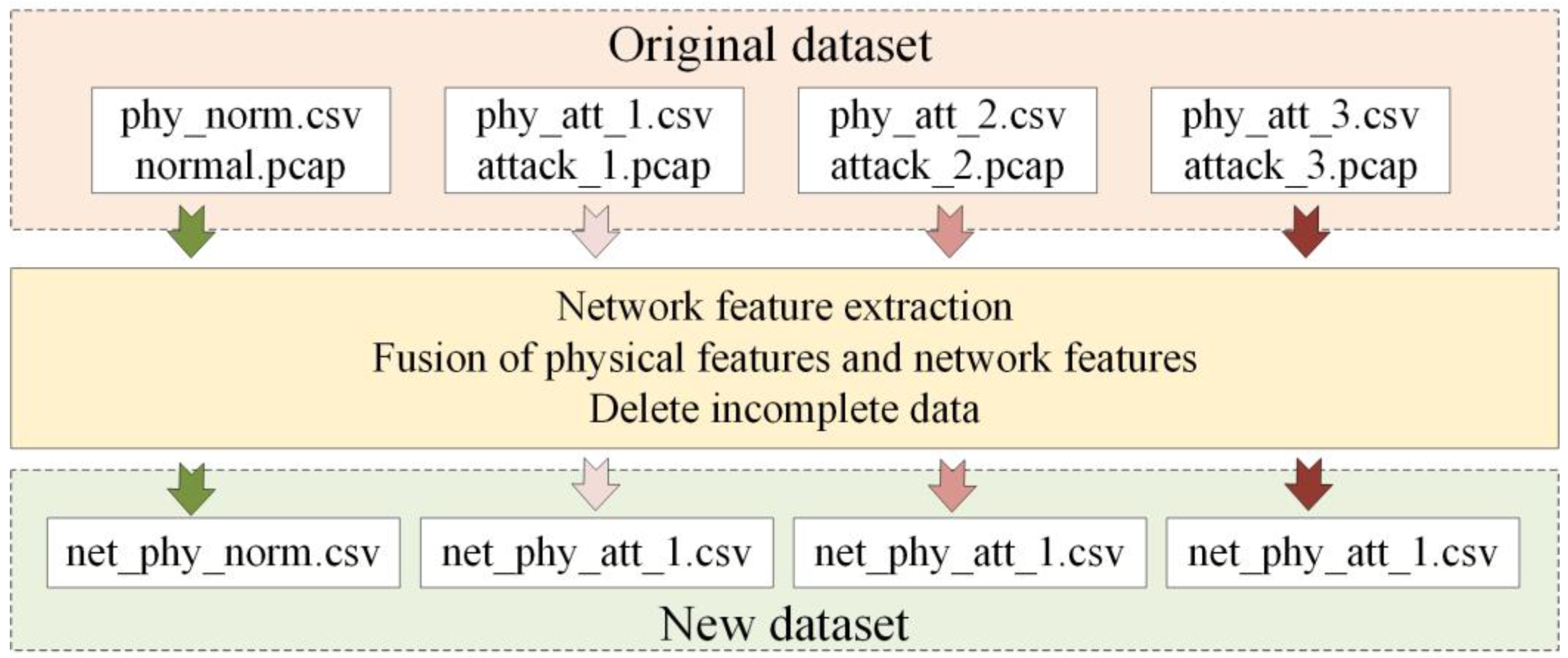
  • Based on the latest public ICS dataset, a method for extracting system network features is designed for ICS, and the original physical features are fused with additionally extracted network features to create a cyber–physical dataset with fusion features.
  • A model is proposed for unsupervised anomaly detection for ICS based on LSTM-Autoencoder and GAN, which is evaluated using the cyber–physical dataset. In terms of precision, recall, and F1-score, the model outperforms several other methods.
  • Both supervised and unsupervised algorithms are used to investigate the effects of additional extracted network features on anomaly detection results. As a result of the experiments performed in this paper, it has been found that the features extracted from the network can significantly improve the performance of the anomaly detection algorithm.
Acquiring data from industrial sensors is an inherent function of ICS, and ICS network traffic data can be collected by listening to communication channels. It is feasible to collect both network data and physical data, and then extract the cyber–physical fusion features. The massive amount of data generated during the normal operation of the ICS is sufficient to train the unsupervised model. Without significantly changing the components of the ICS, the models need to be trained only once to detect anomalies, including various novel attack methods. It is undeniable that the components of an ICS are fixed for a long time, and the network topology is not easily changed. Therefore, the unsupervised anomaly detection model using the cyber–physical fusion features proposed in this paper can help industrial control systems cope with various cyber and physical threats, attacks, and challenges in a cost-effective and profitable manner.
In the remainder of this paper, the following sections are presented: Section 2 discusses related work in the area of anomaly detection of ICS; Section 3 describes the dataset used in this paper; Section 4 describes the method proposed in this paper; Section 5 describes the experimental setup and presents the experimental results and analysis; and Section 6 concludes with our future plans.

2. Related Work

It is necessary to detect anomalies in ICS in order to ensure its security. Studies conducted in the past can be categorized according to their use of physical information or network traffic, depending on the features selected.
(1)
Studies using physical information. Industrial sensors collect physical data such as water level, temperature, and humidity. Ahmed et al. [18] use the hardware characteristics of the sensor and the physical characteristics of the process to create a unique fingerprint for each sensor. In normal operation, noise-based fingerprints are created and can be used to detect attacks by comparing the differences between the noise pattern and the fingerprint pattern. According to Lin et al. [19], timed automata can be used to learn the laws that govern the change of sensor value. Furthermore, sensor and actuator dependencies are analyzed using a Bayesian network. The method is capable of detecting anomalies and locating the abnormal sensor or actuator. Industrial sensor data can be analyzed based on their time and frequency characteristics. In their study, Nguyen et al. [20] developed a method for detecting outliers in time-frequency data using continuous wavelet transforms. The authors of Zhao et al. [21] proposed a correlation-based method for detecting anomalies using sensor data and the correlations between them. Compared with only using sensor data, their method achieved higher accuracy.
(2)
Studies using network traffic. Since ICS networks are more stable than IT networks, abnormal network traffic usually indicates that the system is being attacked. Network traffic-based anomaly detection methods can be further divided into packet-based detection, flow-based detection, and session-based detection [22]. To detect abnormal behavior in ICS, Song et al. [23] extracted the behavioral sequence data from Modbus traffic to model the system’s normal behavior, and compared the actual behavioral data with the model’s predictions. Lee et al. [24] proposed AE-CGAN (autoencoder-conditional GAN) to oversample rare classes on the basis of the GAN model. It is able to achieve more accurate performance metrics in the case of significant imbalance between normal and abnormal traffic. Benaddi et al. [25] used Distributional Reinforcement Learning (DRL) and GAN to help distributional RL-based IDS enhance the detection of minority network attacks and improve the efficiency and robustness of anomaly detection systems in the Industrial Internet of Things (IIoT). By extracting the temporal characteristics of the original traffic in the SCADA system, Kalech et al. [26] proposed a method for detecting network anomalies based on temporal pattern recognition. In order to detect abnormal behavior, Hidden Markov models and artificial neural networks are used. A multi-level anomaly detection scheme combining LSTMs and Bloom filters was proposed by Feng et al. [27] in order to detect malicious traffic in SCADA datasets. An algorithm for detecting anomalous traffic was proposed by Zhang et al. [28]. A grayscale image was created by converting the ICS traffic feature values into grayscale images, and then the model was trained with the resulting grayscale images, which improved the accuracy of anomaly detection.
According to another perspective, past research can also be divided into supervised and unsupervised research. The use of supervised machine learning has been demonstrated in some studies [29,30] as a means of detecting anomalous events or attacks. In spite of good results, the system was only able to detect known attacks and not unknown or zero-day attacks. ICS datasets are also often imbalanced, i.e., the anomalous samples are much smaller than the normal samples, which limits the performance of the supervised algorithm. Unsupervised or semi-supervised algorithms have been used in other studies to overcome the limitations of supervised algorithms. According to Kravchik et al. [31], their algorithm was able to detect 31 out of 36 network attacks using a one-dimensional CNN-based semi-supervised algorithm. Chang et al. [32] reported that an anomaly detection framework based on k-means and convolutional autoencoders achieved an F1-score of 0.9373 for water storage tank datasets. An autoencoder-based anomaly detection model was proposed by Audibert et al. [33], which used the reconstruction error as the loss function during the training phase and as the anomaly score during the testing phase. An anomaly is determined when the sample’s anomaly score exceeds a predetermined threshold. Using an adaptive update strategy based on WGAN-GP, Lu et al. [34] proposed an improved generative adversarial network that produces fake anomaly samples, improving the accuracy of anomaly detection. Li et al.’s [35] GAN-based semi-supervised method, MAD-GAN, utilizes both LSTMs as generators and discriminators to capture the temporal correlation between time series distributions and potential interactions between variables, and it can detect anomalies effectively.
Anomaly detection algorithms are designed based on the selection of appropriate features. In order to detect anomalies in ICS, it is not enough to rely solely on physical information, but it is also necessary to consider network information. However, there are some limitations to the above methods due to the dataset. It was found that the datasets they selected had the following problems: (1) the dataset was not acquired in an ICS environment; (2) the dataset was nonpublic; (3) the dataset was outdated; and (4) the dataset was either restricted to physical process data or to network traffic. The authors in [36] compared the classification performance achieved by the algorithm when only using network features with that achieved by the algorithm when using physical network features, demonstrating that the fusion of physical and network information contributes to improved classification accuracy. The experiment was conducted on four supervised machine learning algorithms, but unsupervised algorithms were not considered.
Due to the above deficiencies, the following improvements have been made in this paper.
  • In terms of the dataset, the latest ICS public dataset WDT [37] is utilized, which provides data on physical processes and their corresponding network traffic.
  • When extracting features, we take into account the physical information and network traffic of ICS.
  • Both supervised and unsupervised algorithms are used in the evaluation of performance to determine whether cyber–physical features contribute to the improvement of anomaly detection.
  • An unsupervised anomaly detection model based on LSTM-Autoencoder and GAN is proposed, which solves the problem of low recall in past anomaly detection models, and is suitable for the ICS field that does not have sufficient labeled samples.

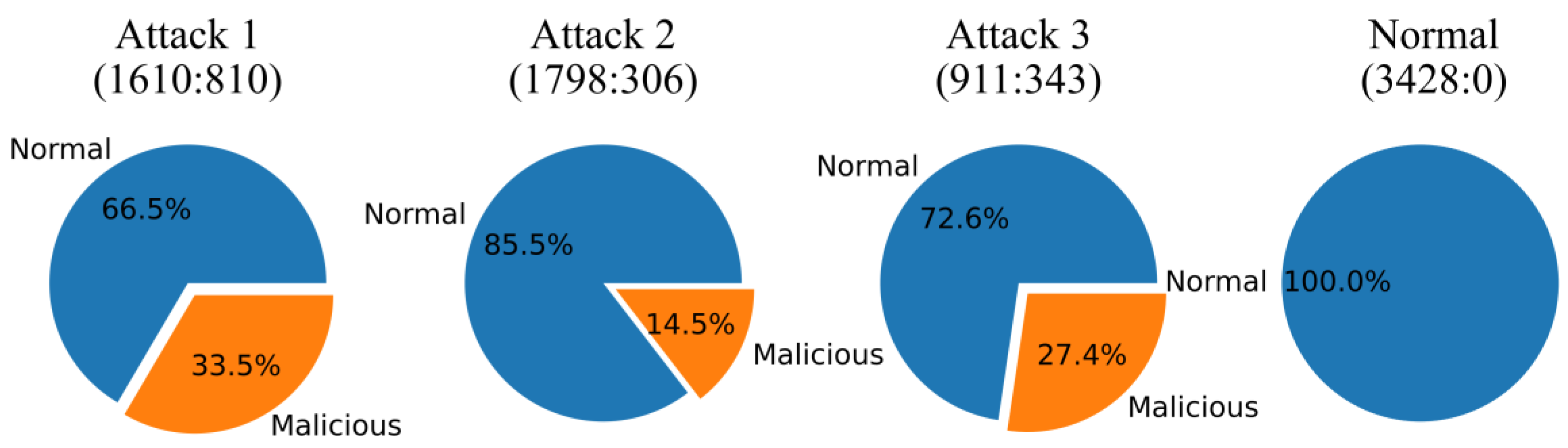
3. Dataset Description

During the normal operation of the Water Distribution Testbed as well as in the event of network attacks or physical faults, the dataset used in this study was compiled from four acquisitions. In Table 1, each acquisition is represented as a sub-dataset. During the first acquisition, eight network attacks or physical failures were conducted, resulting in eight scenarios. In a similar manner, the second and third acquisitions yielded thirteen and seven scenarios, respectively. As of the time of the fourth acquisition, the system was functioning normally, without any network attacks or physical faults. In total, physical faults included two water leaks and six sensors and pumps breakdowns, and network attacks included eight man-in-the-middle (MITM) attacks, five denial of service (DoS) attacks, and seven scanning attacks. Figure 1 shows the number and proportion of samples divided into normal and malicious for each acquisition.
This dataset provides both the physical process data and the corresponding raw network traffic. The physical process data describe the information for the 40 physical statuses of the system in every second, such as whether the pump is turned on and the pressure sensor value of the water tank. In addition, the dataset also provides some network features extracted from raw network traffic data, such as the IP and MAC addresses of packets. For more detailed information on this dataset, please refer to [37].

4. Methodology

Firstly, we describe how to extract additional network features and fuse them with the original physical features. Then we formulate the problem, and finally we describe our proposed anomaly detection model in more detail.

4.1. Extraction and Fusion of Additional Network Features

The physical information collected by industrial sensors alone is not capable of detecting abnormal behavior in time owing to the widespread adoption of traditional information technology in ICS, and the damage caused by cyberattacks has a hysteresis. It is therefore important to take into account both physical information and network traffic when extracting features for anomaly detection.
The original physical process datasets have a sampling interval of one second, while the number of samples collected per second in the original network datasets is over 1000. By re-extracting the network features from the original network traffic according to the specifics of the ICS network, we can fuse the physical and network features together and summarize the situation every second. To enhance the performance of anomaly detection, 22 additional features were extracted from the original dataset. In Table 2, you will find a list of the new features that have been added.
In addition, a feature named stage is added, which describes the stage of the current moment in the process cycle, and its value range is (0,1]. Taking the fourth acquisition as an example, there are a total of 3423 sampling points, including 12 complete process cycles. As shown in Figure 2, in each process cycle, the water level of Tank_1 gradually increases from 0 to the maximum value, and then gradually decreases to 0 and maintains for a period of time. Correspondingly, the value of stage is gradually increased from 0 to 1 and maintained for a period of time.
The architecture of additional feature extraction and fusion is shown in Figure 3. For each row (sample) in the original physical dataset, its sampling time is time t (e.g., 09/04/2021 11:30:55). All packets with time t are aggregated from the network traffic corresponding to this physical dataset, and the features described in Table 2 are extracted from those packets. Subsequently, the newly extracted features are fused with the original physical features to form a cyber–physical dataset. Some incomplete data were deleted, which were mainly concentrated in the first and last part of the dataset. The reason for the incomplete data is that when the original physical dataset is acquired, the corresponding original network dataset has not yet been acquired or the acquisition has been completed. The information of the finally formed cyber–physical dataset is shown in Table 3.

4.2. Problem Formulation
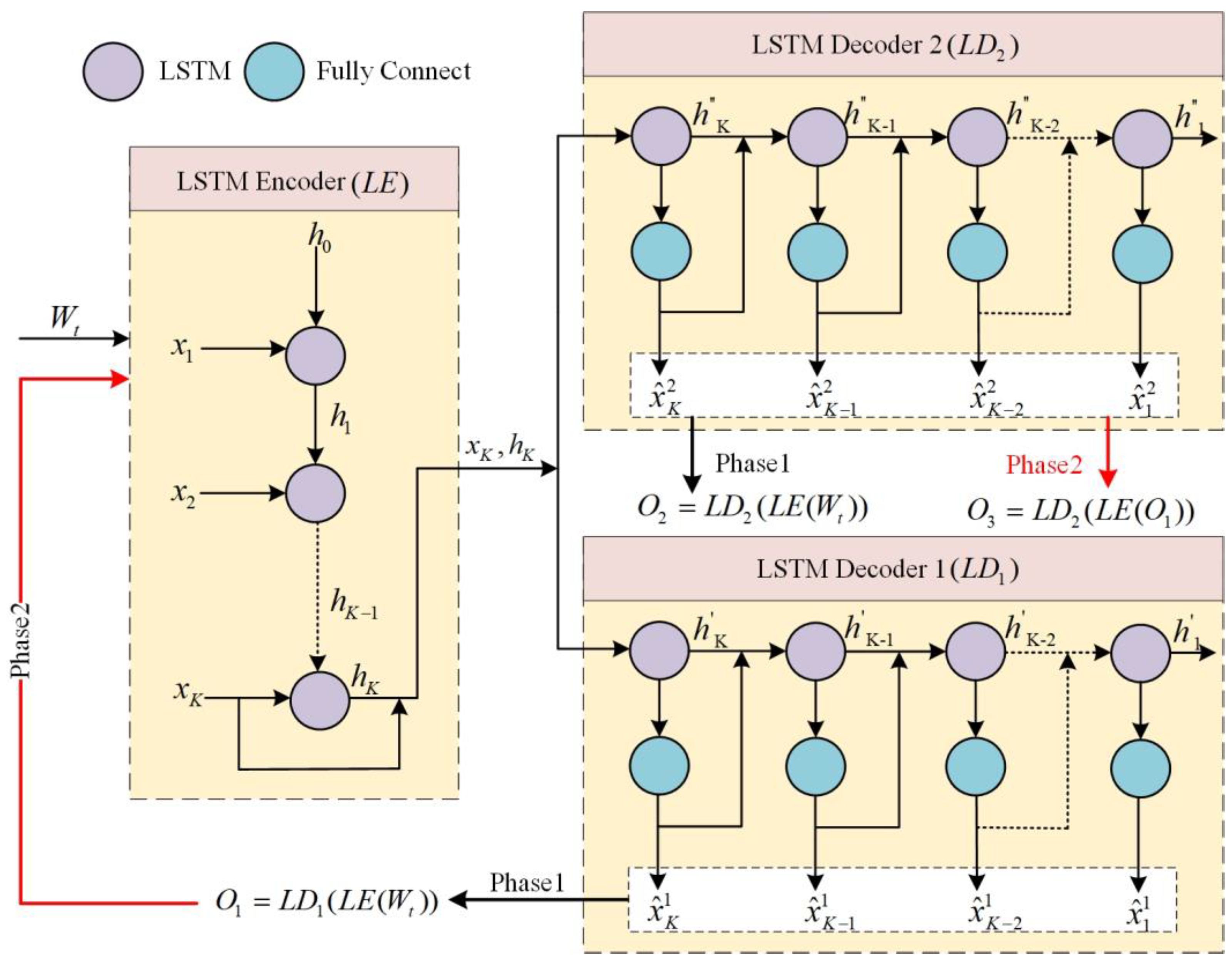
In this paper, a dataset with sample number T is considered a multivariate time series T S of length T. x t is a vector consisting of all physical features and network features at time t, and the number of features is m.
T S = x 1 , x 2 , , x T x t m , 1 t T
In order to make better use of the correlation between observations at the current moment and previous observations, a time window W t is defined. For each observation, its correlation with the previous K observations is considered. Therefore, the original time series T S can be transformed into a time window series W .
W = W 1 , W 2 , , W T ( W t = x t K + 1 , , x t 1 , x t K m , 1 t T )
Use the time window series W as the input to the model instead of the raw time series T S . Before conversion to a time window series, each observation x t in the T S was normalized by
T S j = x 1 j , x 2 j , , x T j x t j = x t j min T S j ε + m a x T S j m i n T S j , 1 j m , 1 t T
where ε is a very small number in order to prevent zero-division.

4.3. Proposed Model

The proposed model consists of three modules: an encoder network L E using LSTM, and two decoder networks L D 1 and L D 2 using LSTM. As can be seen from Figure 4, these three modules constitute two LSTM-Autoencoders L A E 1 and L A E 2 that share the encoder network. The hyperparameters of the model are shown in Table 4. The training of the model consists of two phases.

4.3.1. Phase 1—Input Reconstruction

The goal of this phase is to train L A E 1 and L A E 2 to reconstruct the input. LSTM-Autoencoder can reconstruct each time window W t = x 1 , , x K 1 , x K . The time window W t is used as the input of the model, and the encoder network L E will output the hidden variable h K n (n is the number of cells in the LSTM hidden layer). Then, the two decoder networks will output the reconstructions of W t ( O 1 and O 2 ) according to h K and x K in reverse order, where x K is the last of W t . Use L2-norm to define the reconstruction loss for each decoder:
O 1 = L A E 1 W t , O 2 = L A E 2 W t
L o s s 1 = W t O 1 | | 2 , L o s s 2 = W t O 2 | | 2

4.3.2. Phase 2—Adversarial Training

In the second phase, L A E 1 and L A E 2 are trained adversarially. Put reconstruction O 1 as input to L A E 2 again and output reconstruction O 3 . The purpose of training L A E 2 is to hope that it can distinguish whether O 3 is the real data or a reconstruction of the output of L A E 1 . Conversely, L A E 1 is trained to fool L A E 2 , that is, making L A E 2 unable to judge whether O 3 is the real data. The training objective is:
O 3 = L A E 2 L A E 1 W t
m i n L A E 1 m a x L A E 2 | | W t O 3 | | 2
Therefore, the goal of L A E 1 is to minimize the distance between O 3 and W t , and the goal of L A E 2 is to maximize this distance, and the loss is defined as follows:
L o s s 1 = + W t O 3 | | 2 , L o s s 2 = W t O 3 | | 2
Then, the evolutionary loss function is used to combine the losses of the two phases as the total loss for each LAE.
L o s s 1 = 1 n W t O 1 | | 2 + 1 1 n W t O 3 | | 2
L o s s 2 = 1 n W t O 2 | | 2 1 1 n W t O 3 | | 2
where n denotes the number of training iterations. The training process of the model can be seen in Figure 5a. Now define the anomaly score:
A n o m a l y S c o r e = 1 2 W t O 1 | | 2 + 1 2 W t O 3 | | 2
After the training is completed, the model is used to calculate the anomaly scores for each time window in the normal dataset, and then a threshold is determined based on the distribution of the anomaly scores. During the testing phase, shown in Figure 5b, for each unseen time window, the trained model will output its anomaly score. When the anomaly score of a time window is higher than the threshold, the model judges it as an anomaly.

5. Experiments and Results Analysis

5.1. Experiment Environment and Metrics

The experiments were performed using the following hardware and software platforms: Intel(R) Core (TM) i5-12400 CPU, Windows 10 Professional (64 bits), NVIDIA GeForce GTX 1650 Super, NVIDIA CUDA 11.1, Python 3.7.13, Pytorch 1.8.2, Python Scikit-learn library 1.0.2.
The proposed model is evaluated using recall, precision, F1-score, and accuracy. TP, TN, FP, and FN represent true positive, true negative, false positive, and false negative, respectively.
R e c a l l = T P T P + F N
P r e c i s i o n = T P T P + F P
F 1 s c o r e = 2 × R e c a l l × P r e c i s i o n R e c a l l + P r e c i s i o n
A c c u r a c y = T P + T N T P + F P + F N + T N

5.2. Dataset

The dataset needs to be divided differently for supervised and unsupervised algorithms.

5.2.1. Dataset for Supervised Algorithms

In this paper, the datasets are organized chronologically, with each cyberattack or physical fault lasting for a period of time, corresponding to multiple consecutive samples. When the dataset is shuffled and then divided, some samples from an abnormal event will be placed in the training set, and the remainder will be placed in the testing set. As a result, the model is able to achieve a higher accuracy on the testing set, but this is an illusion [36]. As a result, all samples will be either divided into training sets or testing sets, depending on the scenario. Divide 85% of the normal data into the training set and the rest into the testing set. For the anomaly scenarios, scenario 1.1–1.6, 2.1–2.7, 3.1–3.3 are divided into the training set and the rest are divided into the testing set. Use min–max to normalize the data, and the information of the dataset is shown in Table 5.

5.2.2. Dataset for Unsupervised Algorithms

The fourth acquisition (no anomalies) is used as the training set to train the model. The other three acquisitions (with anomalies) were used as testing sets to evaluate the model.

5.3. Experiments of Using Supervised Algorithms

Three supervised machine learning algorithms were used for training and testing: random forest (RF), support vector machine (SVM), and naïve Bayes (NB). Use RandomForestClassifier, SVC, and GaussianNB in the Python Scikit-learn library to implement the above algorithm, and the hyperparameters for all of the above algorithms are generated by Python Scikit-learn library 1.0.2 defaulted.
The experimental results are shown in Table 6. All three algorithms achieve poor performance when only using physical features. The best performance is achieved by RF, but its F1 score is only 0.28. When using cyber–physical features, the performance achieved by all three algorithms is greatly improved, with F1 scores exceeding 0.87. The results show that the additionally extracted network features can significantly improve the anomaly detection performance of the supervised algorithm.

5.4. Experiments of Unsupervised Algorithms

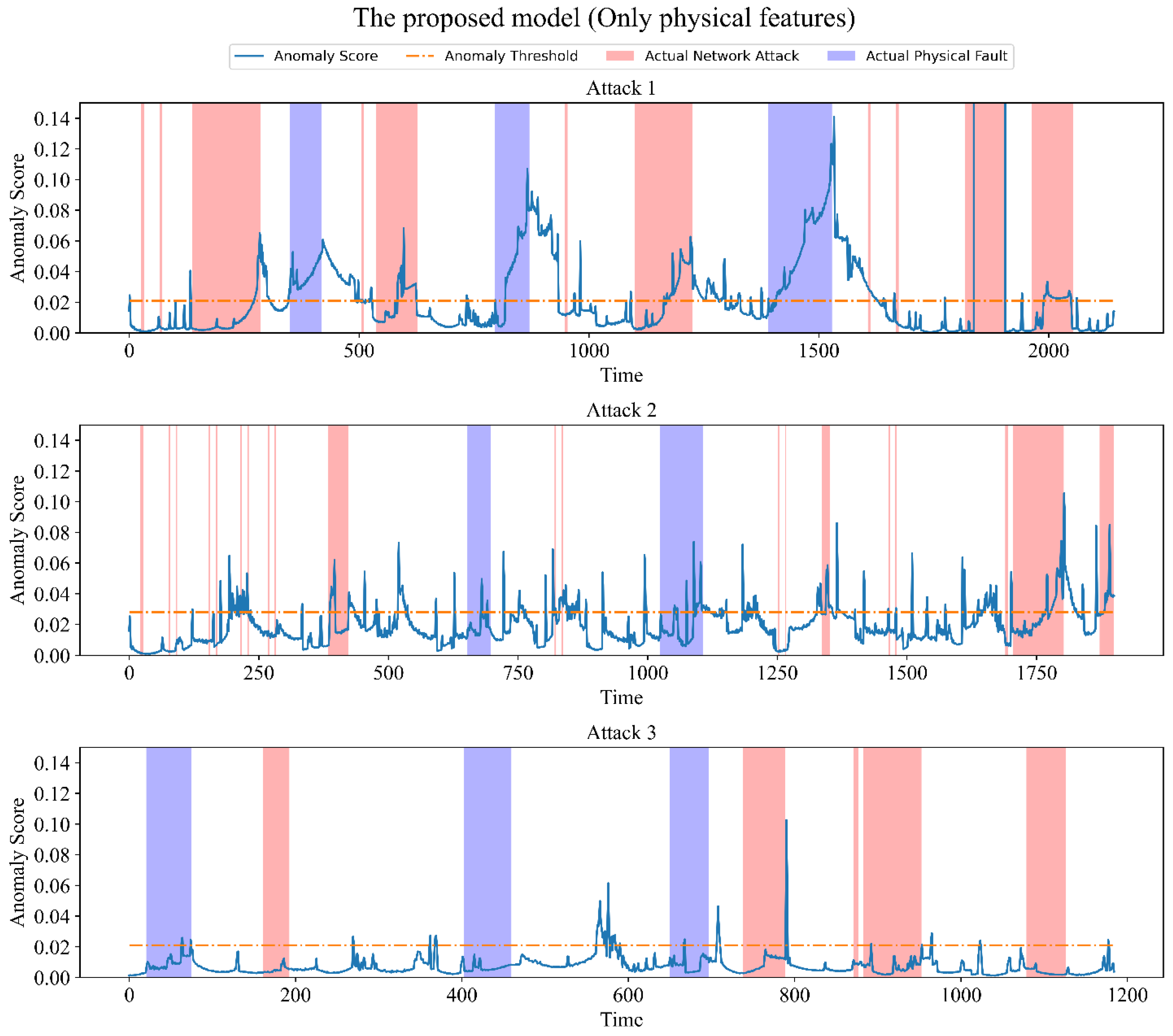
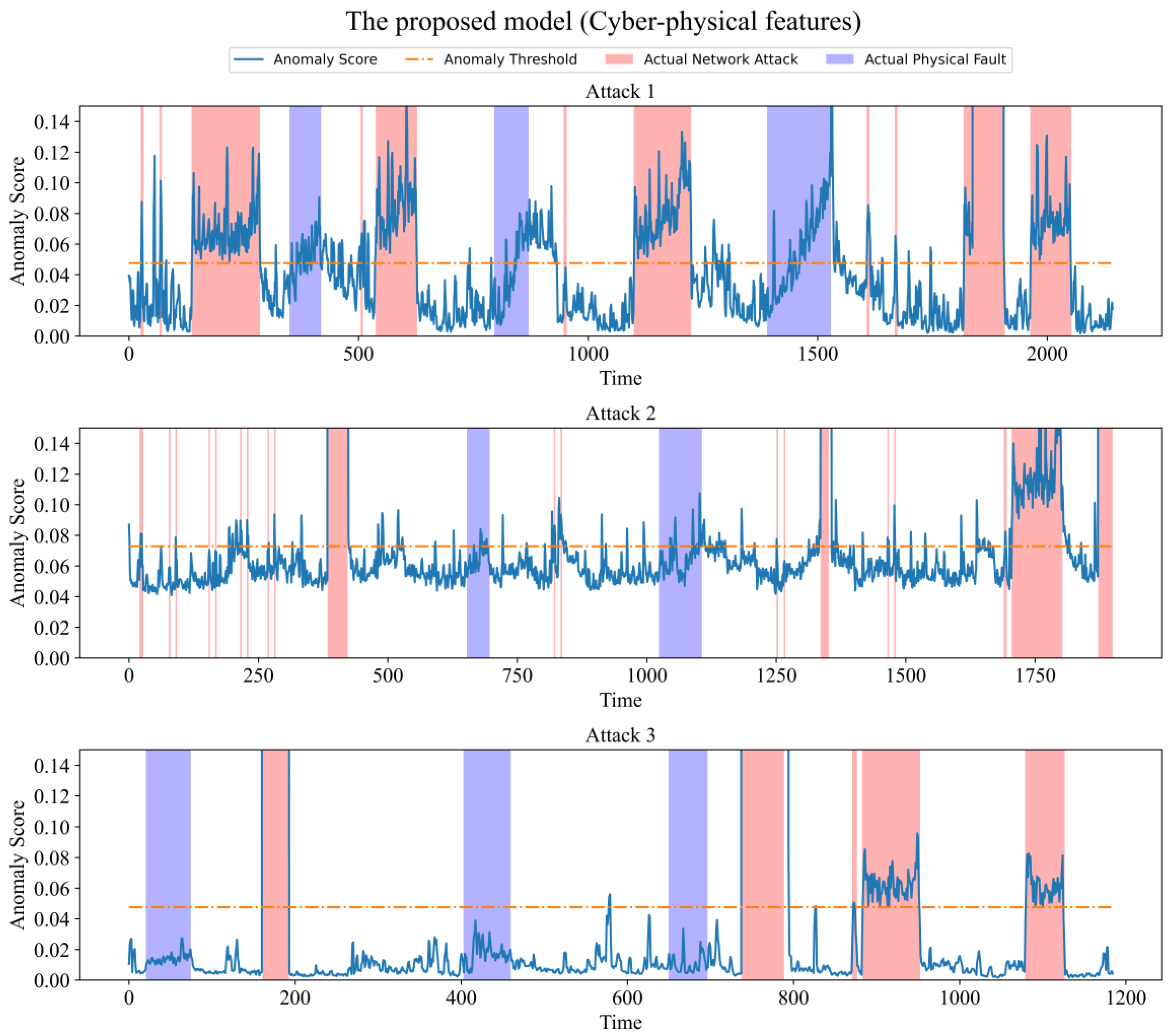
5.4.1. Performance of the Proposed Model

Consider two situations, one using only physical features and another using cyber–physical features. Table 7 shows the performance achieved by the proposed model in the above two situations. In addition, the anomaly scores of the three test sets obtained by the model in the above two situations are shown in Figure 6 and Figure 7, respectively. Cyberattacks and physical faults are marked in red and blue, respectively, in the figure.
When using only physical features, the model performed poorly on all test sets. Conversely, when combining additionally extracted network features, the performance is greatly improved on each test set. We believe that the reason for the poor results obtained by physical features alone is that there are some network attacks that do not affect the physical state of the system too much, so the model fails to detect these network attacks. For the network attack scenario, the anomaly score given by the model for anomalous time points is significantly higher than that for non-anomalous time points, indicating that the model can easily detect network attack events. For physical fault scenarios, the anomaly scores given to anomalous time points are not very significant, but are sufficient to detect most physical fault events.
Due to the continuous increase in the degree of impact of an attack or fault on the system, it may not cause immediate damage to the system at the beginning, resulting in false negatives. Furthermore, it may still take some time for the attacked system to return to normal after the attack has ended, which may result in false positives. An example would be Scenario 1.6, which simulates the rise of the water level in Tank 3 as a result of a leak in the pipeline. A graph of the water level in Tank 3 over time is shown in Figure 8a. Figure 8b shows the corresponding anomaly scores, as well as the time period during which the fault occurred (scenario 1.6). While the water level rose initially, it was consistent with the normal rise in the tank’s level. In this period, the anomaly score does not exceed the threshold, and the model considers it to be a normal period. Persistent faults cause the water level to exceed the normal level and continue to rise. As a result, the anomaly score for this period gradually increases and exceeds the threshold. Upon the resolution of the fault, the water level begins to decline, which is reflected in the anomaly score as well. Nevertheless, the water level remains above the normal level for a period of time after the faults have been resolved, so the anomaly score remains above the threshold, and the model still considers the system to be abnormal.
Figure 9a shows the changes of the water levels of Tank 1 and Tank 5 over time, and Figure 9b shows the corresponding anomaly scores. The time periods of the three fault scenarios are marked by red, green, and blue, respectively. Scenario 3.1 simulates a fault that pauses the transfer of water from Tank 1 to Tank 5. Scenario 3.3 simulates a fault by closing the Tank 5 outlet valve, thus achieving a slowdown in the flow of water from Tank 5. Scenario 3.4 simulates a fault that suspends the transfer of water from the reservoir to Tank 1. None of the above three faults caused the water level to exceed the normal level, so none of the anomaly scores exceeded the threshold and the model considered the system to be in a normal state.

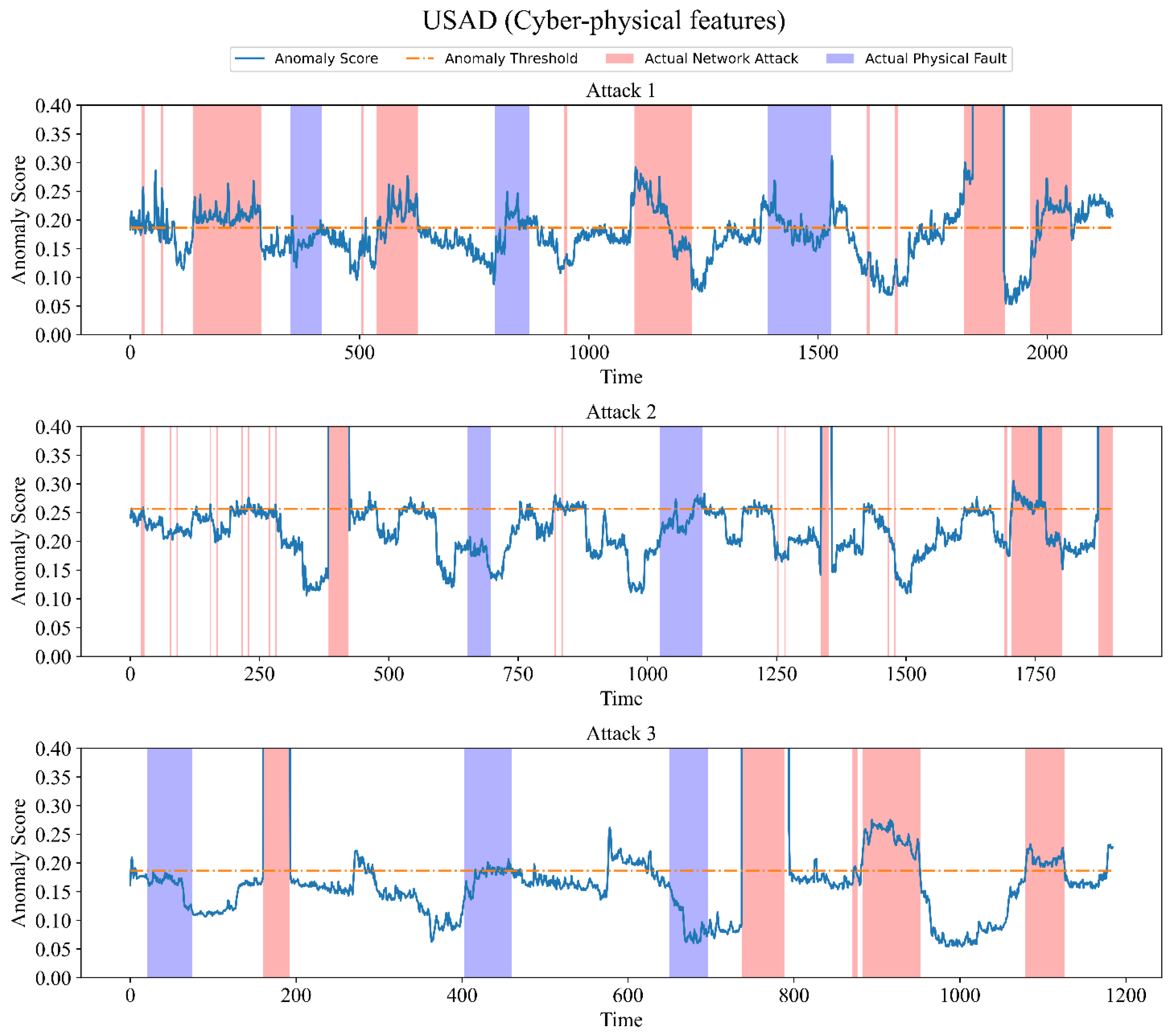
5.4.2. Comparison with Other Unsupervised Algorithms

This section compares the performance of OCSVM [12], Isolation Forest (iForest) [13], USAD [33], and the proposed model. This paper implements USAD based on the author’s GitHub repository. Both One-Class SVM and Isolation Forest are provided by the Python Scikit-learn library and use default parameters.
As can be seen in Table 8, the proposed model outperforms several other algorithms. OCSVM and iForest achieved a high recall rate, but too many false positives resulted in a low F1 score. Compared with the first two algorithms, the F1 score of USAD has been greatly improved, but the recall rate is lower. Low recall means that there are more false negatives, meaning that the model does not effectively detect anomalies, which is fatal for anomaly detection systems. As shown in Figure 10, USAD is able to detect most network attacks, but it is almost incapable of detecting physical faults. In contrast, the proposed model can detect most physical faults. The experimental results show that for the ICS anomaly detection task, the model proposed in this paper can achieve better performance.

5.5. Ablation Experiments
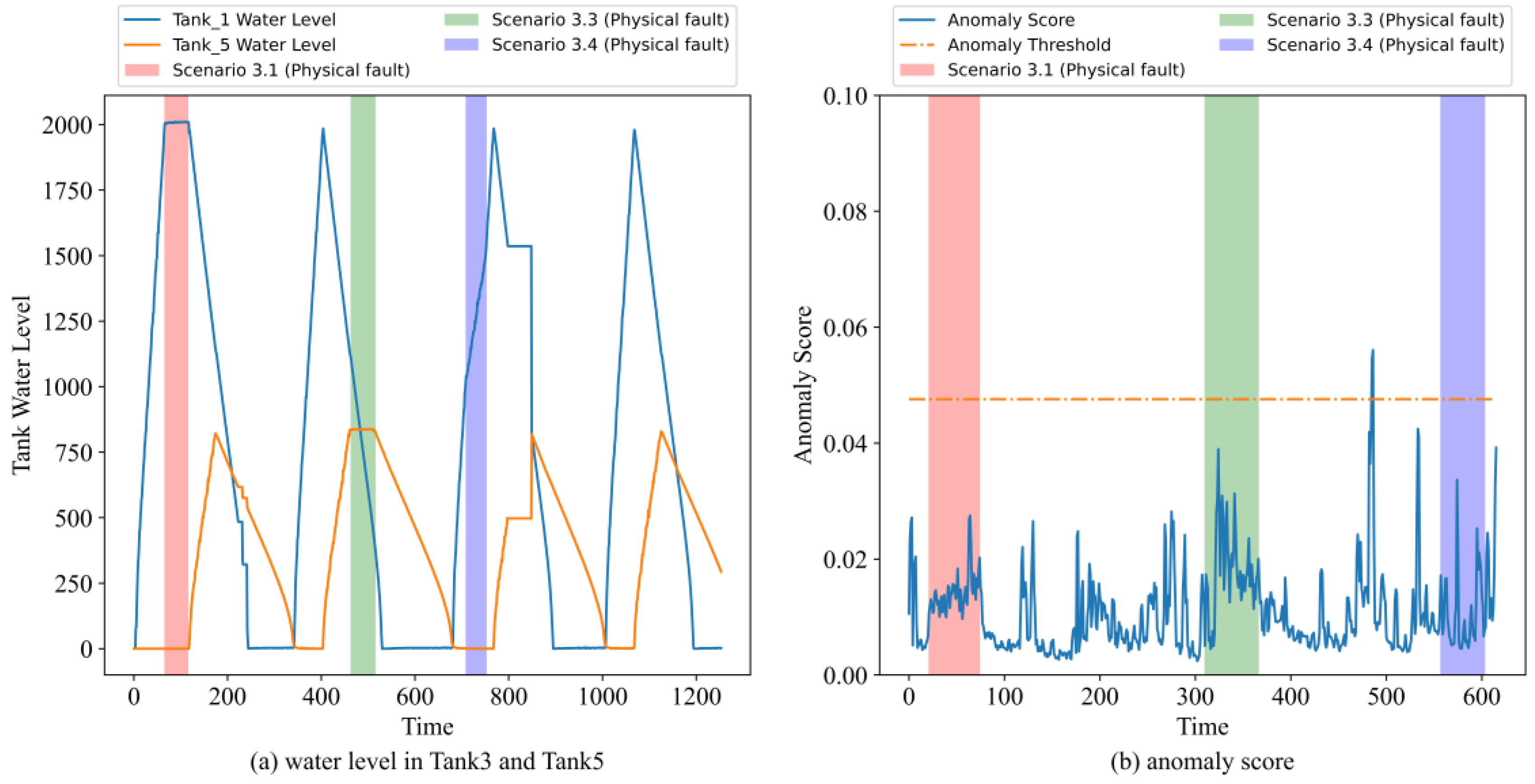
The LSTM autoencoder in the proposed model is replaced by the standard autoencoder, BiLSTM autoencoder, and GRU autoencoder, and their hyperparameters are shown in Table 9. We removed the adversarial training phase from the proposed model, which is hereafter referred to as the proposed model with no adversarial training. The same training settings were set for the above models: the batch size is 32, the window size is 3, the optimizer is Adam, the learning rate is 0.001, the max epoch is 100, and the initial parameters are generated by Pytorch-1.8.2 defaulted.

5.6. Discussion

As shown in Table 6, with the addition of network features, the accuracies of RF, SVM, and NB improved from 0.777, 0.763, and 0.690 to 0.958, 0.953, and 0.945, respectively, and the F1 score, precision, recall, and accuracies of the proposed model improved from 0.425, 0.479, 0.382, and 0.686 to 0.758, 0.800, 0.720, and 0.860, respectively. This is due to the existence of some network attacks, such as scanning attacks, which only generate some anomalous network traffic data, but do not have a substantial impact on the physical conduct of the system. Therefore, the fusion of network traffic data and physical sensor data definitely helps to improve the anomaly detection capability.
Compared with other unsupervised algorithms, the unsupervised anomaly detection model proposed in this paper has better performance. As shown in Table 8, the USAD model achieves a recall of only 0.613 when using cyber–physical fusion features, while the proposed model can improve the recall to 0.720, with a performance improvement of about 17.5%. As can be seen from Figure 7 and Figure 10, the USAD model gives anomaly scores for normal and abnormal data that are not very different in general, which means that it does not reconstruct normal data perfectly and therefore cannot clearly distinguish between normal and abnormal samples. In contrast, the proposed model gives a large difference in the abnormal scores for normal and abnormal data, which indicates that the model can detect abnormalities well.
Table 10 depicts the performance of the standard autoencoder, BiLSTM autoencoder, GRU autoencoder, the proposed model (LSTM autoencoder), and the proposed model with no adversarial training, and Figure 11 shows the time they need to consume for one training. It can be seen that the standard autoencoder achieves the fastest training speed as well as the highest recall rate, but its precision and F1 scores are the lowest. This means that the model identifies numerous normal data as abnormal. The BiLSTM autoencoder took more time to train, but the improvement in performance was marginal. The time cost of training the GRU autoencoder is slightly lower than the time cost of training the proposed model, but the performance of the GRU autoencoder is much worse than the proposed model. It achieves a recall of 0.618, while the proposed model achieves a recall of 0.72, which we believe is worth the small time cost to obtain such a significant improvement. As shown in Figure 12, the model is able to reduce the loss earlier and with smaller loss values when adversarial training is performed. Furthermore, when adversarial training is removed, the recall decreases from 0.72 to 0.652, which is sufficient to demonstrate that adversarial training based on generative adversarial networks is indeed able to identify small anomalies by amplifying the reconstruction error.

6. Conclusions

Given the special characteristics of ICS networks, we designed a method to extract network features. Based on the latest publicly available ICS dataset, the network features are extracted using the previously mentioned method, and then an ICS cyber–physical dataset is created. The anomaly detection algorithm obtained by training with this fused feature has better performance. In addition, we propose an unsupervised anomaly detection method based on LSTM-Autoencoder and GAN. The results of the ablation experiments show that using LSTM as an autoencoder is the optimal choice, and adversarial training based on GAN can also help the model to detect more anomalies.
This paper uses a dataset acquired in ICS using only the Modbus TCP protocol, but other protocols such as S7 and EtherNet/IP exist in the global industry. Our future work will investigate a more effective and compatible method for detecting ICS anomalies based on a more comprehensive dataset.

Author Contributions

Conceptualization, Y.D. and Y.H.; funding acquisition, Y.H. and G.W.; methodology, Y.D. and Y.H.; resources, G.W.; software, Y.D.; validation, Y.H., G.W., and P.H.; writing—original draft, Y.D.; writing—review and editing, G.W. and P.H. All authors have read and agreed to the published version of the manuscript.

Funding

This research was supported by Natural Science Foundation of Sichuan Province (No. 2022NSFSC0557), Foundation of Sichuan Network Culture Research Center (No.WLWH22-18), National Natural Science Foundation of China (No. 62102049, No. 62076042), and Key Research and Development Project of Sichuan (No. 2021YFSY0012, No. 2021YFG0332).

Data Availability Statement

The data presented in this study are openly available in the IEEE DataPort at [10.21227/rbvf-2h90] accessed on 20 November 2022, reference number [37].

Conflicts of Interest

The authors declare no conflict of interest.

References

  1. Siniosoglou, I.; Radoglou-Grammatikis, P.; Efstathopoulos, G.; Fouliras, P.; Sarigiannidis, P. A Unified Deep Learning Anomaly Detection and Classification Approach for Smart Grid Environments. IEEE Trans. Netw. Serv. Manag. 2021, 18, 1137–1151. [Google Scholar] [CrossRef]
  2. Liu, J.; Lin, X.; Chen, X.; Wen, H.; Li, H.; Hu, Y.; Sun, J.; Shi, Z.; Sun, L. ShadowPLCs: A Novel Scheme for Remote Detection of Industrial Process Control Attacks. IEEE Trans. Dependable Secur. Comput. 2022, 19, 2054–2069. [Google Scholar] [CrossRef]
  3. Khan, R.; Maynard, P.; McLaughlin, K.; Laverty, D.M.; Sezer, S. Threat Analysis of BlackEnergy Malware for Synchrophasor based Real-time Control and Monitoring in Smart Grid. In Proceedings of the 4th International Symposium for ICS & SCADA Cyber Security Research, Swindon, UK, 23–25 August 2016; pp. 53–63. [Google Scholar] [CrossRef] [Green Version]
  4. Alladi, T.; Chamola, V.; Zeadally, S. Industrial Control Systems: Cyberattack trends and countermeasures. Comput. Commun. 2020, 155, 1–8. [Google Scholar] [CrossRef]
  5. Fahim, M.; Sillitti, A. Anomaly Detection, Analysis and Prediction Techniques in IoT Environment: A Systematic Literature Review. IEEE Access 2019, 7, 81664–81681. [Google Scholar] [CrossRef]
  6. Ayodeji, A.; Liu, Y.; Chao, N.; Yang, L. A new perspective towards the development of robust data-driven intrusion detection for industrial control systems. Nucl. Eng. Technol. 2020, 52, 2687–2698. [Google Scholar] [CrossRef]
  7. Zhang, M.; Qu, H.; Belatreche, A.; Chen, Y.; Yi, Z. A highly effective and robust membrane potential-driven supervised learning method for spiking neurons. IEEE Trans. Neural Netw. Learn. Syst. 2018, 30, 123–137. [Google Scholar] [CrossRef]
  8. Zhang, M.; Wang, J.; Wu, J.; Belatreche, A.; Amornpaisannon, B.; Zhang, Z.; Miriyala, V.; Qu, H.; Chua, Y.; Carlson, T.; et al. Rectified linear postsynaptic potential function for backpropagation in deep spiking neural networks. IEEE Trans. Neural Netw. Learn. Syst. 2021, 33, 1947–1958. [Google Scholar] [CrossRef]
  9. Huang, Y.; Wang, D.; Sun, Y.; Hang, B. A fast intra coding algorithm for HEVC by jointly utilizing naive Bayesian and SVM. Multimed. Tools Appl. 2020, 79, 33957–33971. [Google Scholar] [CrossRef]
  10. Gou, J.; Sun, L.; Yu, B.; Wan, S.; Ou, W.; Yi, Z. Multi-Level Attention-Based Sample Correlations for Knowledge Distillation. IEEE Trans. Ind. Inform. 2022, 1–11, (early access). [Google Scholar] [CrossRef]
  11. Huang, Y.; Lu, J.; Tang, H.; Liu, X. A Hybrid Association Rule-Based Method to Detect and Classify Botnets. Secur. Commun. Netw. 2021, 2021, 1028878. [Google Scholar] [CrossRef]
  12. Amer, M.; Goldstein, M.; Abdennadher, S. Enhancing one-class support vector machines for unsupervised anomaly detection. In Proceedings of the ACM SIGKDD Workshop on Outlier Detection and Description, Chicago, IL, USA, 11 August 2013; pp. 8–15. [Google Scholar] [CrossRef]
  13. Liu, F.T.; Ting, K.M.; Zhou, Z. Isolation Forest. In Proceedings of the 2008 Eighth IEEE International Conference on Data Mining, Washington, DC, USA, 15–19 December 2008; pp. 413–422. [Google Scholar] [CrossRef]
  14. Bank, D.; Koenigstein, N.; Giryes, R. Autoencoders. arXiv 2020, arXiv:2003.05991. [Google Scholar]
  15. Tuli, S.; Casale, G.; Jennings, N.R. TranAD: Deep Transformer Networks for Anomaly Detection in Multivariate Time Series Data. arXiv 2022, arXiv:2201.07284. [Google Scholar] [CrossRef]
  16. Cai, Z.; Xiong, Z.; Xu, H.; Wang, P.; Li, W.; Pan, Y. Generative Adversarial Networks. ACM Comput. Surv. 2021, 54, 1–38. [Google Scholar] [CrossRef]
  17. Provotar, O.I.; Linder, Y.M.; Veres, M.M. Unsupervised Anomaly Detection in Time Series Using LSTM-Based Autoencoders. In Proceedings of the 2019 IEEE International Conference on Advanced Trends in Information Theory (ATIT), Kyiv, Ukraine, 18–20 December 2019; pp. 513–517. [Google Scholar] [CrossRef]
  18. Ahmed, C.M.; Zhou, J.; Mathur, A.P. Noise matters: Using sensor and process noise fingerprint to detect stealthy cyber attacks and authenticate sensors in cps. In Proceedings of the 34th Annual Computer Security Applications Conference, San Juan, PR, USA, 3–7 December 2018; pp. 566–581. [Google Scholar] [CrossRef] [Green Version]
  19. Lin, Q.; Adepu, S.; Verwer, S.; Mathur, A. TABOR: A graphical model-based approach for anomaly detection in industrial control systems. In Proceedings of the 2018 on Asia Conference on Computer and Communications Security, Incheon, Republic of Korea, 4 June 2018; pp. 525–536. [Google Scholar] [CrossRef]
  20. Nguyen, L.V.; Kapinski, J.; Jin, X.; Deshmukh, J.; Butts, K.; Johnson, T.T. Abnormal Data Classification Using Time-Frequency Temporal Logic. In Proceedings of the 20th International Conference on Hybrid Systems: Computation and Control, Pittsburgh, PA, USA, 18–20 April 2017; pp. 237–242. [Google Scholar] [CrossRef]
  21. Zhao, P.; Kurihara, M.; Tanaka, J.; Noda, T.; Chikuma, S.; Suzuki, T. Advanced correlation-based anomaly detection method for predictive maintenance. In Proceedings of the 2017 IEEE International Conference on Prognostics and Health Management (ICPHM), Dallas, TX, USA, 19–21 June 2017; pp. 78–83. [Google Scholar] [CrossRef]
  22. Liu, H.; Lang, B. Machine Learning and Deep Learning Methods for Intrusion Detection Systems: A Survey. Appl. Sci. 2019, 9, 4396. [Google Scholar] [CrossRef] [Green Version]
  23. Zhanwei, S.; Zenghui, L. Abnormal detection method of industrial control system based on behavior model. Comput. Secur. 2019, 84, 166–178. [Google Scholar] [CrossRef]
  24. Lee, J.; Park, K. AE-CGAN Model based High Performance Network Intrusion Detection System. Appl. Sci. 2019, 9, 4221. [Google Scholar] [CrossRef] [Green Version]
  25. Benaddi, H.; Jouhari, M.; Ibrahimi, K.; Ben Othman, J.; Amhoud, E.M. Anomaly Detection in Industrial IoT Using Distributional Reinforcement Learning and Generative Adversarial Networks. Sensors 2022, 22, 8085. [Google Scholar] [CrossRef]
  26. Kalech, M. Cyber-attack detection in SCADA systems using temporal pattern recognition techniques. Comput. Secur. 2019, 84, 225–238. [Google Scholar] [CrossRef]
  27. Feng, C.; Li, T.; Chana, D. Multi-level Anomaly Detection in Industrial Control Systems via Package Signatures and LSTM Networks. In Proceedings of the 2017 47th Annual IEEE/IFIP International Conference on Dependable Systems and Networks (DSN), Denver, CO, USA, 26–29 June 2017; pp. 261–272. [Google Scholar] [CrossRef] [Green Version]
  28. Zhang, Y.; Li, X.; Li, D.; Yang, H. Abnormal flow monitoring of industrial control network based on convolutional neural network. J. Comput. Appl. 2019, 39, 1512. [Google Scholar] [CrossRef]
  29. Beaver, J.M.; Borges-Hink, R.C.; Buckner, M.A. An Evaluation of Machine Learning Methods to Detect Malicious SCADA Communications. In Proceedings of the 2013 12th International Conference on Machine Learning and Applications, Miami, FL, USA, 4–7 December 2013; pp. 54–59. [Google Scholar] [CrossRef]
  30. Borges Hink, R.C.; Beaver, J.M.; Buckner, M.A.; Morris, T.; Adhikari, U.; Pan, S. Machine learning for power system disturbance and cyber-attack discrimination. In Proceedings of the 2014 7th International Symposium on Resilient Control Systems (ISRCS), Denver, CO, USA, 19–21 August 2013; pp. 1–8. [Google Scholar] [CrossRef]
  31. Kravchik, M.; Shabtai, A. Detecting Cyber Attacks in Industrial Control Systems Using Convolutional Neural Networks. In Proceedings of the 2018 Workshop on Cyber-Physical Systems Security and PrivaCy, Toronto, ON, Canada, 19 October 2018; pp. 72–83. [Google Scholar] [CrossRef]
  32. Chang, C.P.; Hsu, W.C.; Liao, I.E. Anomaly Detection for Industrial Control Systems Using K-Means and Convolutional Autoencoder. In Proceedings of the 2019 International Conference on Software, Telecommunications and Computer Networks (SoftCOM), Split, Croatia, 19–21 September 2019; pp. 1–6. [Google Scholar] [CrossRef]
  33. Audibert, J.; Michiardi, P.; Guyard, F.; Marti, S.; Zuluaga, M.A. USAD: UnSupervised Anomaly Detection on Multivariate Time Series. In Proceedings of the 26th ACM SIGKDD International Conference on Knowledge Discovery & Data Mining, Virtual Event, USA, 6–10 July 2020; pp. 3395–3404. [Google Scholar] [CrossRef]
  34. Lu, H.; Du, M.; Qian, K.; He, X.; Wang, K. GAN-Based Data Augmentation Strategy for Sensor Anomaly Detection in Industrial Robots. IEEE Sens. J. 2022, 22, 17464–17474. [Google Scholar] [CrossRef]
  35. Li, D.; Chen, D.; Jin, B.; Shi, L.; Goh, J.; Ng, S.K. MAD-GAN: Multivariate Anomaly Detection for Time Series Data with Generative Adversarial Networks. In Proceedings of the 28the International conference on artificial neural networks, Munich, Germany, 17–19 September 2020; pp. 703–716. [Google Scholar] [CrossRef] [Green Version]
  36. Müller, N.; Ziras, C.; Heussen, K. Assessment of Cyber-Physical Intrusion Detection and Classification for Industrial Control Systems. arXiv 2022, arXiv:2202.09352. [Google Scholar]
  37. Faramondi, L.; Flammini, F.; Guarino, S.; Setola, R. A Hardware-in-the-Loop Water Distribution Testbed Dataset for Cyber-Physical Security Testing. IEEE Access 2021, 9, 122385–122396. [Google Scholar] [CrossRef]
Figure 1. Number and proportion of samples divided into normal and malicious.
Mathematics 10 04373 g001
Figure 2. Changes of stage value and Tank_1 water level during process cycle.
Mathematics 10 04373 g002
Figure 3. Additional network feature extraction and fusion architecture.
Mathematics 10 04373 g003
Figure 4. Proposed model architecture. The proposed model consists of three modules: an encoder network LE, and two decoder networks L D 1 and L D 2 .
Mathematics 10 04373 g004
Figure 5. Proposed model training and testing flow chart. (a) Training flow chart; (b) testing flow chart.
Mathematics 10 04373 g005
Figure 6. Anomaly scores for the proposed model (using only physical features).
Mathematics 10 04373 g006
Figure 7. Anomaly scores for the proposed model (using cyber–physical features).
Mathematics 10 04373 g007
Figure 8. Scenario 1.6. (a) Water level in Tank 3; (b) anomaly score.
Mathematics 10 04373 g008
Figure 9. Scenario 3.1, 3.3, 3.4. (a) Water level in Tank 3 and Tank 5; (b) anomaly score.
Mathematics 10 04373 g009
Figure 10. Anomaly scores for USAD (using network and physical features).
Mathematics 10 04373 g010
Figure 11. Training time for proposed model and other models.
Mathematics 10 04373 g011
Figure 12. Loss with adversarial training and without adversarial training.
Mathematics 10 04373 g012
Table 1. Data acquisition and description.
AcquisitionsDescription
(Scenario Number: 1.1–1.8, 2.1–2.13, 3.1–3.7)
First
(Attack 1)
phy_att_1.csv, attack_1.pcap
5 MITM attack scenarios. (1.1, 1.3, 1.5, 1.7, 1.8)
3 physical fault scenarios. (1.2, 1.4, 1.6)
Second
(Attack 2)
phy_att_2.csv, attack_2.pcap
7 scan attack scenarios. (2.1, 2.2, 2.3, 2.4, 2.7, 2.9, 2.11)
3 Dos attack scenarios. (2.5, 2.10, 2.13)
2 physical fault scenarios. (2.6, 2.8)
1 MITM attack scenarios. (2.12)
Third
(Attack 3)
phy_att_3.csv, attack_3.pcap
3 physical fault scenarios. (3.1, 3.3, 3.4)
2 Dos attack scenarios. (3.2, 3.5)
2 MITM attack scenarios. (3.6, 3.7)
Fourth
(Normal)
phy_normal.csv, normal.pcap
No attack.
Table 2. Additional extracted features.
No.FeaturesDescription
1pkt_numNumber of all types of packets
2icmp_pkt_numNumber of ICMP packets
3arp_pkt_numNumber of ARP packets
4tcp_pkt_numNumber of TCP packets
5mb_q_numNumber of MODBUS request packets
6mb_r_numNumber of MODBUS response packets
7avg_pkt_sizeAverage packet byte size
8avg_payload_sizeAverage packet payload byte size
9mb_q_avgAverage MODBUS request packet payload byte size
10mb_r_avgAverage MODBUS response packet payload byte size
11illegal_macIllegal MAC address appears
12illegal_ipIllegal IP address appears
13fc1_pkt_numNumber of Modbus packets with function code 1
14fc3_pkt_numNumber of Modbus packets with function code 3
15fc5_pkt_numNumber of Modbus packets with function code 5
16fc6_pkt_numNumber of Modbus packets with function code 6
17fin_flag_numNumber of packets with FIN in the TCP flag
18syn_flag_numNumber of packets with SYN in the TCP flag
19rst_flag_numNumber of packets with RST in the TCP flag
20psh_flag_numNumber of packets with PSH in the TCP flag
21ack_flag_numNumber of packets with ACK in the TCP flag
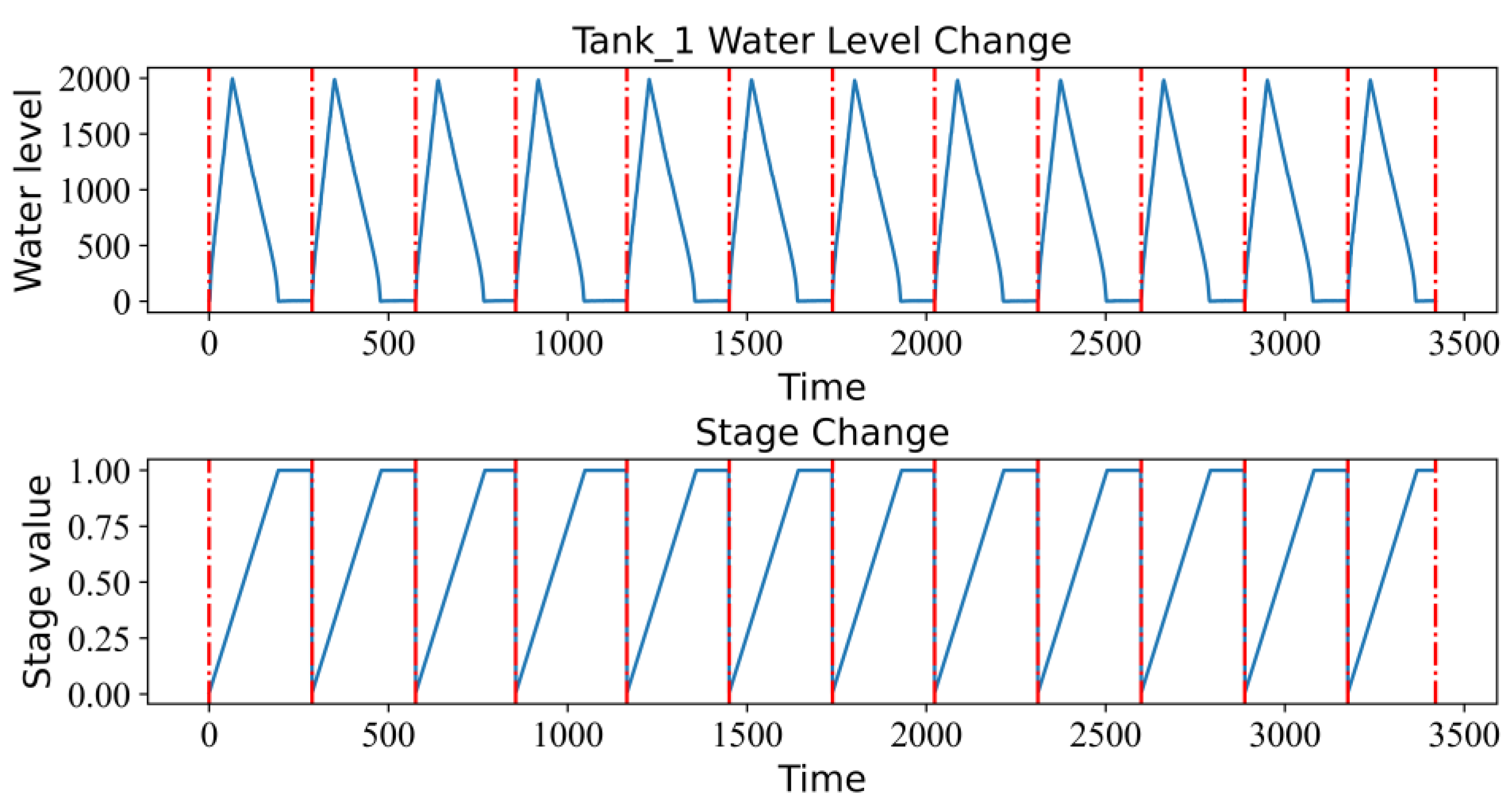
22stageStage of the current moment in a process cycle
Table 3. Cyber–physical dataset after feature fusion.
DatasetNumber of Samples and Features
net_phy_att_1.csv(2409, 62)
net_phy_att_2.csv(2092, 62)
net_phy_att_3.csv(1248, 62)
net_phy_norm.csv(3421, 62)
Total samples9170
Table 4. Model hyperparameters.
ModuleHyperparameterValue
LSTM encoderLayer of LSTM1
Input size and hidden size for each layer of LSTM(62, 128)
Dropout0.2
LSTM decoder1
and
LSTM decoder2
Layer of LSTM1
Input size and hidden size for each layer of LSTM(62, 128)
Dropout0.2
Layer of Dense1
Size of each layer of the Dense(128, 62)
Table 5. Dataset information for supervised algorithms.
LabelTraining SetTesting Set
Normal58481864
Physical fault426385
MITM358126
DoS6789
Scan52
Total67042466
Table 6. Performance of three supervised machine learning algorithms.
AlgorithmPhysical FeaturesCyber–Physical Features
F1PRAF1PRA
RF0.2570.7540.1550.7770.9071.0000.8310.958
SVM0.1260.7640.0680.7630.8951.0000.8090.953
NB0.1960.2760.1510.6900.8780.9820.7950.945
Table 7. Performance of the proposed model.
AcquisitionPhysical FeaturesCyber–Physical Features
F1PRAF1PRA
Attack 10.5740.5740.5740.6570.8270.8270.8260.860
Attack 20.2920.2930.2920.7300.6460.6460.6450.865
Attack 30.0290.1430.0160.6670.6920.9570.5420.851
Sum0.4250.4790.3820.6860.7580.8000.7200.860
Table 8. Performance comparison of the proposed model with other methods.
MethodsF1PRA
OC-SVM0.4890.3240.9990.364
iForest0.4840.3410.8340.458
USAD0.6220.6320.6130.774
Proposed model0.7580.8000.7200.860
Table 9. Three autoencoder hyperparameters.
CategoryHyperparameterValue
Standard
autoencoder
EncoderLayer of Dense2
Size of the Dense
(W means window size)
(62 × W, 128)
(128, 64)
Dropout, Activation function0.1, ReLu
DecoderLayer of Dense2
Size of the Dense
(W means window size)
(64, 128)
(128, 62 × W)
Dropout, Activation function0.1, ReLu
BiLSTM
autoencoder
EncoderLayer of BiLSTM1
Input size and hidden size for each layer of BiLSTM(62, 128)
Dropout0.2
Layer of BiLSTM1
DecoderInput size and hidden size for each layer of BiLSTM(62, 128)
Dropout0.2
Layer of Dense1
Size of each layer of the Dense(128, 62)
GRU
autoencoder
EncoderLayer of GRU1
Input size and hidden size for each layer of GRU(62, 128)
Dropout0.2
Layer of GRU1
DecoderInput size and hidden size for each layer of GRU(62, 128)
Dropout0.2
Layer of Dense1
Size of each layer of the Dense(128, 62)
Table 10. Performance comparison of LSTM autoencoder with others.
CategoryF1PRA
Standard autoencoder0.5680.4140.9030.581
BiLSTM autoencoder0.7670.8430.7030.870
GRU autoencoder0.7290.8880.6180.860
LSTM autoencoder
(proposed model)
0.7580.8000.7200.860
Proposed model with no adversarial training0.7300.8280.6520.853
Publisher’s Note: MDPI stays neutral with regard to jurisdictional claims in published maps and institutional affiliations.

