Article

Global Stability for a Diffusive Infection Model with Nonlinear Incidence

by
Xiaolan Liu
1,†,
Cheng-Cheng Zhu
2,*,
Hari Mohan Srivastava
3,4,5,6,† and
Hongyan Xu
7,†
1
School of Arts and Science, Suqian University, Suqian 223800, China
2
School of Science, Jiangnan University, Wuxi 214122, China
3
Department of Mathematics and Statistics, University of Victoria, Victoria, BC V8W 3R4, Canada
4
Department of Medical Research, China Medical University Hospital, China Medical University, Taichung 40402, Taiwan
5
Department of Mathematics and Informatics, Azerbaijan University, AZ197 Baku, Azerbaijan
6
Section of Mathematics, International Telematic University Uninettuno, I-00186 Rome, Italy
7
College of Arts and Sciences, Suqian University, Suqian 223800, China
*
Author to whom correspondence should be addressed.
These authors contributed equally to this work.
Mathematics 2022, 10(22), 4296; https://doi.org/10.3390/math10224296
Submission received: 11 October 2022 / Revised: 10 November 2022 / Accepted: 11 November 2022 / Published: 16 November 2022
(This article belongs to the Section Mathematical Physics)

Abstract

:
The first purpose of this article was to establish and analyze system 4 with an abstract function incidence rate under homogeneous Neumann boundary conditions. The system models the dynamics of interactions between pathogens and the host immune system, which has important applications in HIV-1, HCV, flu etc. By the Lyapunov–LaSalle method, we obtained the globally asymptotic stability of the equilibria. Specifically speaking, by introducing the reproductive numbers R 0 and R 1 , we showed that if R 0 1 , then the infection-free equilibrium E 0 is globally asymptotically stable, i.e., the virus is unable to sustain the infection and will become extinct; if R 1 1 < R 0 , then the C T L -inactivated infection equilibrium E 1 is globally asymptotically stable, i.e., the infection becomes chronic but without persistent CTL response; if R 1 > 1 , the C T L -activated equilibrium E 2 is globally asymptotically stable, and the infection is chronic with persistent CTL response. Additionally, we also investigate the discretization of the model by using a non-standard finite difference scheme, and our results confirm that the global stability of the equilibria of the continuous model and the discrete model is consistent. Finally, numerical simulations are performed to illustrate the theoretical results. Our model and results are to a certain extent generalizations of and improvements upon the previous results given by Zhu, Wang.

1. Introduction

In recent decades, epidemic models have been proposed not only to properly study epidemics but also to predict the behavior of biological systems or social phenomena. The SIR model was introduced for the first time in 1927 (Kermack and McKendrick 1927), of which many variations have since been proposed to study diseases with complex behaviors and other phenomena. In recent years, with the new coronavirus pandemic affecting the whole world, virus dynamics has again become a hot spot. Environmental factors, such as humidity and temperature, have significant impacts on the spread of the new strain of coronavirus COVID-19 to humans (see [1,2]); people are increasingly worried about the impact of the virus on lives (see [3,4]). Many mathematical models of host virus dynamics have been developed. There were a lot of references focusing on the dynamics of interactions between pathogens and the host immune system using computer models (can refer to [5,6,7,8,9,10]).
A virus cannot replicate on its own, so it must take over host cells and use them to replicate. Once invaded by viruses, these infected cells will produce a cytotoxic T-lymphocyte (CTL) response from the immune system, and hence many scholars have examined various CTL dynamics (see [11,12]).
Epidemic models have been applied to express the dynamics inside the host of various infectious diseases such as HCV, HIV-1, flu, or even the malaria parasite. As many of the diseases caused by them, e.g., hepatitis B and AIDS, are chronic and incurable, some different mechanisms of the immune system are of interest [13].
To date, many scholars have paid increasing interest to infection models with cell-mediated immune response. Now, let us recall some results about the model of immune response during a viral infection. Researchers first considered the interaction between a replicating virus and host cells in [14,15,16]:
{ x ˙ = λ d x β x v , y ˙ = β x v a y , v ˙ = k y μ v ,
where variables x , y , v denote the uninfected cells, infected cells, and free virus particles, respectively. λ and β x v stand for the recruitment rate of the uninfected cells and infected cells, respectively. d x and a y represent the death rates of uninfected cells and infected cells, respectively. The free virus is produced at rate k y and removed at rate μ v .
To help the body heal, cytotoxic T-lymphocyte effectors (CTLe) of the immune system will decrease the infected cells to prevent further viral replications. In order to model these extra dynamics, researchers extended (1) to the system describing immune responses with infected cells:
x ˙ = λ d x β x v , y ˙ = β x v a y , v ˙ = k y μ v s . , z ˙ = c y z b z ,
where variable z stands for the magnitude of the C T L response and c y z denotes the rate of C T L proliferation in response to antigen. Due to the lack of stimulation, C T L s declines at a rate of b z . C T L s clear infected cells at rate p y z .
The time delay model is widely used in different fields of application in mathematical biology, e.g., epidemic models ([1,2]). Later, Zhu and Zou [17] in 2009 and Wang and Guan [18] in 2012 studied a mathematical model with cell-mediated immune response and intracellular delay:
d x ( t ) d t = λ d x ( t ) β x v , d y ( t ) d t = e a τ β x ( t τ ) v ( t τ ) a y ( t ) p y ( t ) z ( t ) , d v ( t ) d t = k y ( t ) μ v ( t ) , d z ( t ) d t = c y ( t ) z ( t ) b z ( t ) .
In [17], by analyzing equilibria, the local stability of E 1 and E 2 is obtained, but the global stability of both equilibria is left. In the present paper, we show that the global dynamics are fully determined. In [18], the global dynamics for (3) is discussed, but the model is particular. However, there is no diffusion term in the model. It is known that the virus is not stationary in space (can refer to [19,20,21,22]). The model can be generalized. By discussing the evolution of the model (1)–(3), the following questions can be raised naturally.
Question 1. 
What can be said about the diffusion term in (3)?
Question 2. 
What can be said about the infection with a general nonlinear incidence rate?
Question 3. 
How to select the proper discrete scheme such that it can efficiently preserve the global dynamics of solutions of the corresponding continuous models?
In [23], a susceptible–infected–susceptible epidemic reaction–diffusion model governed by a mass action infection mechanism and linear birth–death growth with no flux boundary condition was investigated. In [24], an attraction–repulsion Keller–Segel system with homogeneous Neumann boundary conditions in a bounded domain with a smooth boundary was considered. By constructing a Lyapunov function, the global existence of uniformly-in-time bounded classical solutions with large initial data if the repulsion dominates or cancels attraction was established. The movement of the virus in space generates the spatial spread of the disease. Fickian diffusion can reasonably represent the spread of this virus in space and the Laplace operator can represent this diffusion process. Hence, in this paper, we extend the previous model to a diffusive infection model with intracellular delay and cell-mediated immune response:
T ( x , t ) t = λ d T ( x , t ) β 1 T ( x , t ) f ( V ( x , t ) ) β 2 T ( x , t ) g ( I ( x , t ) ) , I ( x , t ) t = e a τ ( β 1 T ( x , t τ ) f ( V ( x , t τ ) ) + β 2 T ( x , t τ ) g ( I ( x , t τ ) ) ) a I ( x , t ) p I ( x , t ) Z ( x , t ) , V ( x , t ) t = d 1 Δ V ( x , t ) + k I ( x , t ) μ V ( x , t ) , Z ( x , t ) t = c I ( x , t ) Z ( x , t ) b Z ( x , t ) ,
here, T ( x , t ) , I ( x , t ) , V ( x , t ) , Z ( x , t ) denote the densities of uninfected cells, infected cells, virus, and C T L s at position x at time t, respectively. The parameter λ is the natural produce rate, d is the death rate of the susceptible cells. a represents the death rate for infected but not even virus-producing cells. The virus is instantaneously generated at a rate of k. Virus particles are derived from the model at a rate of μ . Parameter p stands for the strength of the lytic component and b is the death rate for C T L s , d 1 is the diffusion coefficient and Δ is the Laplace operator. c I ( x , t ) Z ( x , t ) denotes the production of C T L s . Delay τ stands for the lag between the time between the moment the virus comes into contact with a target cell and the cell becomes actively infected. The probability of surviving from time t τ to time t is e a τ . Here, forms β 1 T f ( V ) and β 2 T g ( I ) stand for the nonlinear incidences of the responses to the concentrations of virus particles and infected cells, where f ( V ) and g ( I ) represent the strength of infection by virus and infected cells that satisfies [25]:
f ( 0 ) = g ( 0 ) = 0 , f ( V ) > 0 , g ( I ) > 0 , f ( V ) 0 , g ( I ) 0 .
In combination with ( A 1 ) and the mean value theorem, we can obtain
f ( V ) V f ( V ) f ( 0 ) V , g ( I ) I g ( I ) g ( 0 ) I , f o r I , V 0 .
From an epidemiological view, condition (5) makes it clear that: ( 1 ) if there is no infection, the disease cannot spread; ( 2 ) the incidences β 1 T f ( V ) and β 2 T g ( I ) become faster if the densities of the virus and infected cells increase; ( 3 ) as (6) implies that ( f ( V ) V ) 0 and ( g ( I ) I ) 0 , then the per capita infection rates by virus particles and infected cells will reduce from a certain inhibiting effect. It is obvious that the incidence rate with (5) implies the bilinear and the saturation incidences.
In the present paper, we study the system (4) with initial conditions as
T ( x , s ) = ϕ 1 ( x , s ) 0 , I ( x , s ) = ϕ 2 ( x , s ) 0 , V ( x , s ) = ϕ 3 ( x , s ) 0 , Z ( x , s ) = ϕ 4 ( x , s ) 0 , ( x , s ) Ω ¯ × [ τ , 0 ] ,
and homogeneous Neumann boundary conditions
V n = 0 , t > 0 , x Ω .
where Ω is a bounded, connected domain in R n with a smooth boundary Ω , and V n represents the outward normal derivative on Ω .
Generally, it is difficult or even impossible to ensure the exact solution for system (1). Hence, in a number of previous articles [26,27,28,29,30,31,32,33,34,35,36], some mathematicians described the forms of entire solutions of several functional equations or systems, and scholars looked for a numerical one instead. However, choosing the proper discrete scheme remains an open problem [37], such that it has the same global dynamics as the corresponding continuous models. In fact, Mickens has made an attempt, by providing a robust non-standard finite difference (NSFD) scheme [38]. Now, it has been widely used in some epidemic systems [39,40]. Motivated by the work of [38,41,42,43], we applied the NSFD scheme to discretize system (4) and obtain:
T n + 1 m T n m Δ t = λ d T n + 1 m β 1 T n + 1 m f ( V n m ) β 2 T n + 1 m g ( I n m ) , I n + 1 m I n m Δ t = e a τ ( β 1 T n m 1 + 1 m f ( V n m 1 m ) + β 2 T n m 1 + 1 m g ( I n m 1 m ) ) a I n + 1 m p I n + 1 m Z n m , V n + 1 m V n m Δ t = d 1 V n + 1 m + 1 2 V n + 1 m + V n + 1 m 1 ( Δ x ) 2 + k I n + 1 m μ V n + 1 m , Z n + 1 m Z n m Δ t = c I n + 1 m Z n m b Z n + 1 m ,
here, we set x Ω = [ a , b ] , and Δ t > 0 denotes the time step size, N is the positive integer, and Δ x = b a N stands for the space step size. Suppose that m 1 N with τ = m 1 Δ t . { ( x m , t n ) , m = 0 , 1 , 2 , , N , n N + } denotes the mesh grid point with x m = a + m Δ x and t n = n Δ t . Denote approximations of T ( x m , t n ) , I ( x m , t n ) , V ( x m , t n ) , Z ( x m , t n ) by ( T n m , I n m , V n m , Z n m ) . U n = ( U n 0 , U n 1 , , U n N ) T stands for all the approximation solutions at time t n , where U { T , I , V , Z } and ( · ) T denotes the transposition of a vector. U 0 means that all components of a vector U are non-negative. The discrete initial conditions of system (9) are given as
T s m = ϕ 1 ( x m , t s ) 0 , I s m = ϕ 2 ( x m , t s ) 0 , V s m = ϕ 3 ( x m , t s ) 0 , Z s m = ϕ 4 ( x m , t s ) 0 ,
for all s = m 1 , m 1 + 1 , , 0 , and the discrete boundary conditions are given by
V n 1 = V n 0 , V n N = V n N + 1 , for n N .
Then, we will show that the discretized system (9) can efficiently preserve the global asymptotic stability of equilibria to the continuous system (4), if it is derived by using the NSFD scheme. The paper is structured as: in Section 2.1, we introduced one new model under some assumptions, and obtained that the positive property and bounded property of the solutions of the model. In Section 2.2, we discuss the existence of equilibria of our model mentioned in Section 2.1. In Section 2.3, we analyze the global stability of the model. In particular, we prove that the global stability of the corresponding equilibria under the conditions of the cases R 0 1 , R 1 1 < R 0 and R 1 > 1 , respectively. In Section 3, by using a non-standard finite difference scheme, we investigate the global dynamics of the discrete system (9) and confirm that the global dynamics of the discrete system are consistent with the continuous system (4). Moreover, we give some numerical simulations to illustrate our analytical results in Section 4. Finally, the conclusion and the discussion in Section 5 outline the direction of our future work.

2. Dynamical Behaviors of System (4)

2.1. Positivity and Boundedness of Solutions

Let X = C ( Ω ¯ , R 4 ) be the space of continuous functions from the topological space Ω ¯ into the space R 4 . Let C = C ( [ τ , 0 ] , X ) be the Banach space of continuous functions from [ τ , 0 ] into X with the usual supremum normal. An element ϕ C means that a function from Ω ¯ × [ τ , 0 ] into R 4 as
ϕ ( x , s ) = ϕ ( s ) ( x ) .
Define x t ( s ) = x ( t + s ) , s [ τ , 0 ] , for any continuous function x ( · ) : [ τ , σ ) X for σ > 0 , then t x t is a continuous function from [ 0 , σ ) to C .
Theorem 1. 
For any ϕ C ,
(a) 
System (4)–(8) has a unique solution; and
(b) 
The solution of (4)–(8) is non-negative and bounded for all t 0 .
Proof. 
For any ϕ = ( ϕ 1 , ϕ 2 , ϕ 3 , ϕ 4 ) T C and x Ω ¯ , let
F = ( F 1 , F 2 , F 3 , F 4 ) : C X
by
F 1 ( ϕ ) ( x ) = λ d ϕ 1 ( x , 0 ) β 1 ϕ 1 ( x , 0 ) f ϕ 3 ( x , 0 ) β 2 ϕ 1 ( x , 0 ) g ϕ 2 ( x , 0 ) , F 2 ( ϕ ) ( x ) = e a τ β 1 ϕ 1 ( x , τ 1 ) f ϕ 3 ( x , τ 1 ) + β 2 ϕ 1 ( x , τ 1 ) g ϕ 2 ( x , τ 1 ) a ϕ 2 ( x , 0 ) p ϕ 2 ( x , 0 ) ϕ 4 ( x , 0 ) , F 3 ( ϕ ) ( x ) = k ϕ 2 ( x , τ 2 ) μ ϕ 3 ( x , 0 ) , F 4 ( ϕ ) ( x ) = c ϕ 2 ( x , 0 ) ϕ 4 ( x , 0 ) b ϕ 4 ( x , 0 ) .
Then, system (4)–(8) can be rewritten as
U ( t ) = A U + F ( U t ) , t > 0 , U ( 0 ) = ϕ X .
Here U = ( T , I , V , Z ) T , ϕ = ( ϕ 1 , ϕ 2 , ϕ 3 , ϕ 4 ) T and A U = ( 0 , 0 , d 1 Δ V , 0 ) T . It is obvious that the operator F is locally Lipschitz in space X. From [22,44,45,46,47,48], the system (11) has a unique local solution on t [ 0 , T m a x ) , where T m a x is the maximal existence time for the solution of system (4). It follows from that 0 is a sub-solution of each equation of system (4), then T ( x , t ) 0 , I ( x , t ) 0 , V ( x , t ) 0 , Z ( x , t ) 0 .
Next, we prove the boundedness of the solutions. Assume that
G 1 ( x , t ) = e μ 1 τ 1 T ( x , t τ 1 ) + I ( x , t ) + p c Z ( x , t ) ,
then
G 1 ( x , t ) t = λ e a τ d e a τ T ( x , t τ 1 ) a I ( x , t ) p b c Z ( x , t ) λ d ˜ G 1 ( x , t ) ,
where d ˜ = m i n { a , b , d } , then
G 1 ( x , t ) m a x λ d ˜ , max x Ω ¯ e a τ ϕ 1 ( x , τ 1 ) + ϕ 2 ( x , 0 ) + p c ϕ 3 ( x , 0 ) = ξ 1 .
Thus, T ( x , t ) , I ( x , t ) and Z ( x , t ) are bounded.
From the boundedness of I ( x , t ) and system (4)–(8), V ( x , t ) satisfies the following
V t d 1 Δ V k ξ 1 μ V , V n = 0 , V ( x , 0 ) = ϕ 3 ( x , 0 ) 0 .
Assume that V 1 ( t ) is a solution to the system
d V 1 d t = k ξ 1 μ V 1 , V 1 ( 0 ) = max x Ω ¯ ϕ 3 ( x , 0 ) .
then
V 1 ( t ) max k ξ 1 μ , max x Ω ¯ ϕ 3 ( x , 0 ) , t [ 0 , T m a x ) .
According to the comparison principle [49], we obtain that V ( x , t ) V 1 ( t ) . Therefore
V ( x , t ) m a x k ξ 1 μ , max x Ω ¯ ϕ 3 ( x , 0 ) = ξ 2 , ( x , t ) Ω ¯ × [ 0 , T m a x ) .
From the above, T ( x , t ) , I ( x , t ) , V ( x , t ) and Z ( x , t ) are bounded in Ω ¯ × [ 0 , T m a x ) . Then, it follows from the standard theory for semilinear parabolic systems [50] that T m a x = + . □

2.2. Existence of Equilibria

Clearly, system (4) always has an infection-free equilibrium E 0 = ( T 0 , 0 , 0 , 0 ) , where T 0 = λ d , corresponding to the maximal level of healthy C D 4 + T cells. It is the only biological meaningful equilibrium if
R 0 = λ e a τ ( k β 1 f ( 0 ) + μ β 2 g ( 0 ) ) a d μ < 1 ,
which denotes the basic reproduction number.
An equilibrium of model (4) satisfies
λ = d T + β 1 T f ( V ) + β 2 T g ( I ) , e a τ ( β 1 T f ( V ) + β 2 T g ( I ) ) = a I + p I Z , k I = μ V , c I Z = b Z .
If Z = 0 , a short calculation reduces that
λ d T = a μ e a τ k V , I = μ k V .
To ensure that T 0 and V > 0 , we have V ( 0 , k λ a μ e a τ ] . From the second equation of (2),
T = a μ e a τ k ( β 1 f ( V ) + β 2 g ( μ k V ) ) V ,
we substitute T into the first equation of (2)
λ = a d μ e a τ k ( β 1 f ( V ) + β 2 g ( μ k V ) ) V + a μ e a τ k V = H ( V ) .
For all V > 0 , according to (6)
H ( V ) = a d μ e a τ ( β 1 ( f ( V ) V f ( V ) ) + β 2 ( g ( μ k V ) μ V k g ( μ k V ) ) ) k ( β 1 f ( V ) + β 2 g ( μ k V ) ) 2 + a μ e a τ k > 0 .
Furthermore, from (5) we have
lim V 0 + H ( V ) = a d μ e a τ k ( β 1 f ( 0 ) + μ β 2 g ( 0 ) = λ R 0 ,
and
H ( k λ a μ e a τ ) = λ + λ d β 1 f ( k λ a μ e a τ ) + β 2 g ( λ a e a τ ) > λ .
This implies that if R 0 > 1 , then there is an infection equilibrium without immunity E 1 = ( T 1 , I 1 , V 1 , 0 ) .
Define
R 1 = c λ e a τ ( β 1 f ( k b μ c ) + β 2 g ( b c ) ) a b ( d + β 1 f ( k b μ c ) + β 2 g ( b c ) ) ,
R 1 stands for the immune response activation number and determines whether a persistent immune response can be established. If Z 0 , then from (2), we have
T 2 = λ d + β 1 f ( k b μ c ) + β 2 g ( b c ) , I 2 = b c , V 2 = k b μ c , Z 2 = a p ( R 1 1 ) .
Then, if R 1 > 1 , the infection equilibrium with immunity E 2 = ( T 2 , I 2 , V 2 , Z 2 ) exists. Concluding the above analysis, we have the following results.
Lemma 1. 
For system (4):
(1) 
There is a unique infection-free equilibrium E 0 , when R 0 < 1 .
(2) 
There is a unique infection equilibrium without immunity E 1 besides E 0 , when R 1 1 < R 0 .
(3) 
There is a unique infection equilibrium with immunity E 2 besides E 0 and E 1 , when R 1 > 1 .

2.3. Global Asymptotic Stability

By constructing Lyapunov functionals, we establish the global asymptotic stability of the system (4). Assume φ ( u ) = u 1 ln u for u ( 0 , + ) , then φ : R + R + has strict global minimum φ ( 1 ) = 0 .
Theorem 2. 
If R 0 1 , then the infection-free equilibrium E 0 is globally asymptotically stable.
Proof. 
Let
L 1 = Ω T 0 φ T T 0 + e a τ I + β 1 T 0 f ( 0 ) R 0 μ V + p e a τ c Z + + t τ t [ β 1 T ( s ) f ( V ( s ) ) + β 2 T ( s ) g ( I ( s ) ) ] d s d x .
Then, L 1 0 , calculating d L 1 d t along the solutions of system (4) and using λ = d T 0 , we obtain
d L 1 d t = Ω 1 T 0 T ( x , t ) [ d T 0 T ( x , t ) ( d + β 1 f ( V ( x , t ) ) + β 2 g ( I ( x , t ) ) ) ] + T ( x , t τ ) [ β 1 f ( V ( x , t τ ) ) + β 2 g ( I ( x , t τ ) ) ] e a τ I ( x , t ) [ a + p Z ( x , t ) ] + [ d 1 Δ V ( x , t ) + k I ( x , t ) μ V ( x , t ) ] β 1 T 0 f ( 0 ) R 0 μ + T ( x , t ) [ β 1 f ( V ( x , t ) ) + β 2 g ( I ( x , t ) ) ] T ( x , t τ ) [ β 1 f ( V ( x , t τ ) ) + β 2 g ( I ( x , t τ ) ) ] + [ c I ( x , t ) b ] Z ( x , t ) p e a τ c d x ,
noting that Ω Δ v ( x , t ) d x = 0 , we have
d L 1 d t = Ω 1 T 0 T ( x , t ) ( d T 0 d T ( x , t ) ) ( 1 T 0 T ( x , t ) ) ( β 1 T ( x , t ) f ( V ( x , t ) ) + β 2 T ( x , t ) g ( I ( x , t ) ) e a τ I ( x , t ) + β 1 T 0 f ( 0 ) k R 0 μ I ( x , t ) β 1 T 0 f ( 0 ) R 0 V ( x , t ) b p e a τ c Z ( x , t ) + β 1 T ( x , t ) f ( V ( x , t ) ) + β 2 T ( x , t ) g ( I ( x , t ) ) d x .
It follows from the expression of R 0 and condition (6) that
a e a τ β 1 k T 0 f ( 0 ) e a τ R 0 μ = β 2 T 0 g ( 0 ) R 0 ,
and
d L 1 d t = Ω d T ( x , t ) ( T ( x , t ) T 0 ) 2 + β 1 T 0 f ( V ( x , t ) ) + β 2 T 0 g ( I ( x , t ) ) β 2 T 0 g ( 0 ) R 0 I ( x , t ) β 1 T 0 f ( 0 ) R 0 V ( x , t ) b p e a τ c Z ( x , t ) d x
Ω d T ( x , t ) ( T ( x , t ) T 0 ) 2 + β 1 T 0 f ( 0 ) R 0 ( R 0 1 ) V ( x , t ) + β 2 T 0 g ( 0 ) R 0 ( R 0 1 ) I ( x , t ) b p e a τ c Z ( x , t ) d x .
It is clear that d L 1 d t 0 when R 0 1 . Furthermore, the largest invariant subset of { d L 1 d t = 0 } is the singleton { E 0 } . Thus, it follows from LaSalle’s invariance principle that E 0 is globally asymptotically stable. □
Theorem 3. 
If R 1 1 < R 0 , then C T L -inactivated infection equilibrium E 1 is globally asymptotically stable.
Proof. 
Constructing a Lyapunov functional
L 2 = Ω T 1 φ ( T T 1 ) + e a τ I 1 φ ( I I 1 ) + β 1 T 1 f ( V 1 ) k I 1 V 1 φ ( V V 1 ) + β 1 T 1 f ( V 1 ) t τ t φ T ( θ ) f ( V ( θ ) ) T 1 f ( V 1 ) d θ + β 2 T 1 g ( I 1 ) t τ t φ T ( θ ) g ( I ( θ ) ) T 1 g ( I 1 ) d θ + p e a τ c Z d x .
Calculating d L 2 d t along the solutions of system (4), we have
d L 2 d t = Ω 1 T 1 T ( x , t ) [ λ T ( x , t ) ( d + β 1 f ( V ( x , t ) ) + β 2 g ( I ( x , t ) ) ) ] + 1 I 1 I ( x , t ) T ( x , t τ ) [ ( β 1 f ( V ( x , t τ ) ) + β 2 g ( I ( x , t τ ) ) ) e a τ I ( x , t ) [ a + p Z ( x , t ) ] + β 1 T 1 f ( V 1 ) k I 1 1 V 1 V ( x , t ) [ d 1 Δ V ( x , t ) + k I ( x , t ) μ V ( x , t ) ] + β 1 T 1 f ( V 1 ) T ( x , t ) f ( V ( x , t ) ) T 1 f ( V 1 ) T ( x , t τ ) f ( V ( x , t τ ) ) T 1 f ( V 1 ) + ln T ( x , t τ ) f ( V ( x , t τ ) ) T f ( V ) + β 2 T 1 g ( I 1 ) T ( x , t ) g ( I ( x , t ) ) T 1 g ( I 1 ) T ( x , t τ ) g ( I ( x , t τ ) ) T 1 g ( I 1 ) + ln T ( x , t τ ) g ( I ( x , t τ ) ) T g ( I ) + [ c I ( x , t ) b ] Z ( x , t ) p e a τ c d x .
By using the equilibrium conditions of E 1
λ = d T 1 + β 1 T 1 f ( v 1 ) + β 2 T 1 g ( I 1 ) , β 1 T 1 f ( v 1 ) + β 2 T 1 g ( I 1 ) = e a τ a I 1 , k I 1 = μ V 1 ,
recalling that Ω Δ V ( x , t ) = 0 and Ω Δ V ( x , t ) V ( x , t ) d x = Ω V ( x , t ) 2 V 2 ( x , t ) d x , so that
d L 2 d t = Ω d T 1 1 T 1 T ( x , t ) 1 T ( x , t ) T 1 + 1 T 1 T ( x , t ) × β 1 T 1 f ( V 1 ) + β 2 T 1 g ( I 1 ) β 1 T ( x , t ) f ( V ( x , t ) ) β 2 T ( x , t ) g ( I ( x , t ) ) + 1 I 1 I ( x , t ) T ( x , t τ ) [ β 1 f ( V ( x , t τ ) ) + β 2 g ( I ( x , t τ ) ) ] e a τ 1 I 1 I ( x , t ) I ( x , t ) [ a β 2 T ( x , t τ ) g ( I ( x , t τ ) ) + p Z ( x , t ) ] + β 1 T 1 f ( V 1 ) 1 V 1 V ( x , t ) I ( x , t ) I 1 V ( x , t ) I 1 + T ( x , t ) f ( V ( x , t ) ) T 1 f ( V 1 ) T ( x , t τ ) f ( V ( x , t τ ) ) T 1 f ( V 1 ) + ln T ( x , t τ ) f ( V ( x , t τ ) ) T ( x , t ) f ( V ( x , t ) ) + β 2 T 1 g ( I 1 ) T ( x , t ) g ( I ( x , t ) ) T 1 g ( I 1 ) T ( x , t τ ) g ( I ( x , t τ ) ) T 1 g ( I 1 ) + ln T ( x , t τ ) g ( I ( x , t τ ) ) T ( x , t ) g ( I ( x , t ) ) + p e a τ Z ( x , t ) [ I ( x , t ) b c ] d x β 1 T 1 f ( V 1 ) d 1 V 1 k I 1 e a τ Ω V ( x , t ) 2 V 2 ( x , t ) d x = Ω d T 1 1 T 1 T ( x , t ) 1 T ( x , t ) T 1 + β 1 T 1 f ( V 1 ) φ T 1 T ( x , t ) φ T ( x , t τ ) f ( V ( x , t τ ) ) I 1 T 1 f ( V 1 ) I ( x , t ) φ V 1 I ( x , t ) I 1 V ( x , t ) φ f ( V 1 ) V f ( V ) V 1 + f ( V ) f ( V 1 ) V V 1 1 f ( V 1 ) f ( V ) + β 2 T 1 g ( I 1 ) φ T 1 T ( x , t ) φ T ( x , t τ ) g ( I ( x , t τ ) ) I 1 T 1 g ( I 1 ) I φ g ( I 1 ) I g ( I ) I 1 + g ( I ) g ( I 1 ) I I 1 1 g ( I 1 ) g ( I ) + ( I 1 I 2 ) p e a τ Z ( x , t ) d x β 1 T 1 f ( V 1 ) d 1 V 1 k I 1 e a τ Ω V ( x , t ) 2 V 2 ( x , t ) d x .
From (5), it is easy to obtain that
f ( V ) f ( V 1 ) V V 1 1 f ( V 1 ) f ( V ) 0 ,
g ( I ) g ( I 1 ) I I 1 1 g ( I 1 ) g ( I ) 0 .
Furthermore, φ ( u ) 0 for u > 0 , similar to [42], s g n ( I 1 I 2 ) = s g n ( R 1 1 ) , so we have d L 2 d t 0 ; hence E 1 is stable, and d L 2 d t = 0 holds if and only if T ( x , t ) = T 1 , I 1 = I 1 , V = V 1 and z = 0 when R 1 < 1 or T ( x , t ) = T 1 , I 1 = I 1 , V = V 1 when R 1 = 1 . The largest invariance set in { d L 2 d t = 0 } is the singleton { E 1 } . The classical LaSalle’s invariance principle shows that E 1 is globally asymptotically stable when R 1 1 < R 0 . This completes the proof. □
Theorem 4. 
If R 1 > 1 , then the interior equilibrium E 2 is globally asymptotically stable.
Proof. 
Constructing a Lyapunov functional L 3 as follows
L 3 = Ω T 2 φ T T 2 + e a τ I 2 φ I I 2 + β 1 T 2 f ( V 2 ) k I 2 V 2 φ V V 2 + Z 2 p e a τ c φ Z Z 2 + β 1 T 2 f ( V 2 ) t τ t φ T ( θ ) f ( V ( θ ) ) T 2 f ( V 2 ) d θ + β 2 T 2 g ( I 2 ) t τ t φ T ( θ ) g ( I ( θ ) ) T 2 g ( I 2 ) d θ d x .
Calculating d L 3 d t along the solutions of system (4), we have
d L 3 d t = Ω 1 T 2 T ( x , t ) λ T ( x , t ) [ d + β 1 f ( V ( x , t ) ) + β 2 g ( I ( x , t ) ) ]
+ 1 I 2 I ( x , t ) T ( x , t τ ) [ β 1 f ( V ( x , t τ ) ) + β 2 g ( I ( x , t τ ) ) ] e a τ ( 1 I 2 I ( x , t ) ) [ a + p Z ( x , t ) ] I ( x , t ) + β 1 T 2 f ( V 2 ) 1 V 2 V ( x , t ) d 1 k I 2 Δ V ( x , t ) + I ( x , t ) I 2 V ( x , t ) V 2 + p e a τ c 1 Z 2 Z ( x , t ) [ c I ( x , t ) b ] Z ( x , t )
+ β 1 T 2 f ( V 2 ) T ( x , t ) f ( V ( x , t ) ) T 2 f ( V 2 ) T ( x , t τ ) f ( V ( x , t τ ) ) T 2 f ( V 2 ) + ln T ( x , t τ ) f ( V ( x , t τ ) ) T ( x , t ) f ( V ( x , t ) ) + β 2 T 2 g ( I 2 ) T ( x , t ) g ( I ( x , t ) ) T 2 g ( I 2 ) T ( x , t τ ) g ( I ( x , t τ ) ) T 2 g ( I 2 ) + ln T ( x , t τ ) g ( I ( x , t τ ) ) T ( x , t ) g ( I ( x , t ) ) d x .
By using the equilibrium conditions of E 2
λ = d T 2 + β 1 T 2 f ( V 2 ) + β 2 T 2 g ( I 2 ) , k I 2 = μ V 2 ,
β 1 T 2 f ( V 2 ) + β 2 T 2 g ( I 2 ) = e a τ ( a I 2 + p I 2 Z 2 ) , I 2 = b c ,
also recalling Ω Δ V ( x , t ) = 0 , and Ω Δ V ( x , t ) V ( x , t ) d x = Ω V ( x , t ) 2 V 2 ( x , t ) d x , we have
d L 3 d t = Ω d T 2 1 T 2 T ( x , t ) 1 T ( x , t ) T 2 + β 1 T 2 f ( V 2 ) 3 T 2 T ( x , t ) T ( x , t τ ) f ( V ( x , t τ ) ) I 2 T 2 f ( V 2 ) I ( x , t ) V 2 I ( x , t ) I 2 V ( x , t ) + f ( V ) f ( V 2 ) V V 2 + ln T ( x , t τ ) f ( V ( x , t τ ) ) T ( x , t ) f ( V ( x , t ) ) + β 2 T 2 g ( I 2 ) 2 T 2 T ( x , t ) T ( x , t τ ) g ( I ( x , t τ ) ) I 2 T 2 g ( I 2 ) I + g ( I ) g ( I 2 ) I I 2 + ln T ( x , t τ ) g ( I ( x , t τ ) ) T ( x , t ) g ( I ( x , t ) ) d x β 1 T 2 f ( V 2 ) d 1 V 2 k I 2 Ω V ( x , t ) 2 V 2 ( x , t ) = Ω d T 2 1 T 2 T ( x , t ) 1 T ( x , t ) T 2 + β 1 T 2 f ( V 2 ) φ T 2 T ( x , t ) φ T ( x , t τ ) f ( V ( x , t τ ) ) I 2 T 2 f ( V 2 ) I ( x , t ) φ V 2 I ( x , t ) I 2 V ( x , t ) + f ( V ) f ( V 2 ) V V 2 + ln f ( V 2 ) V ( x , t ) V 2 f ( V ( x , t ) ) + β 2 T 2 g ( I 2 ) φ T 2 T ( x , t ) φ T ( x , t τ ) g ( I ( x , t τ ) ) I 2 T 2 g ( I 2 ) I + g ( I ) g ( I 2 ) I I 2 + ln g ( I 2 ) I ( x , t ) I 2 g ( I ( x , t ) ) d x β 1 T 2 f ( V 2 ) d 1 V 2 k I 2 Ω V ( x , t ) 2 V 2 ( x , t ) = Ω d T 2 1 T 2 T ( x , t ) 1 T ( x , t ) T 2 + β 1 T 2 f ( V 2 ) × φ T 2 T ( x , t ) φ T ( x , t τ ) f ( V ( x , t τ ) ) I 2 T 2 f ( V 2 ) I ( x , t ) φ V 2 I ( x , t ) I 2 V ( x , t ) φ f ( V 2 ) V ( x , t ) V 2 f ( V ( x , t ) ) + f ( V ) f ( V 2 ) V V 2 1 f ( V 2 ) f ( V ) + β 2 T 2 g ( I 2 ) × φ T 2 T ( x , t ) φ T ( x , t τ ) g ( I ( x , t τ ) ) I 2 T 2 g ( I 2 ) I φ g ( I 2 ) I ( x , t ) I 2 g ( I ( x , t ) ) + g ( I ) g ( I 2 ) I I 2 1 g ( I 2 ) g ( I ) d x β 1 T 2 f ( V 2 ) d 1 V 2 k I 2 Ω V ( x , t ) 2 V 2 ( x , t ) .
According to (5), it is easy to see that
f ( V ) f ( V 1 ) V V 1 1 f ( V 1 ) f ( V ) 0 ,
g ( I ) g ( I 1 ) I I 1 1 g ( I 1 ) g ( I ) 0 .
Furthermore, φ ( u ) 0 for u > 0 , it is easy to see that d L 3 d t 0 , similar to the proof of Theorem 3. The Lyapunov–LaSalle invariance principle guarantees that solutions converge to the largest invariant set { d L 3 d t = 0 } , and that the largest invariant set consists of the single point { E 2 } . Thus, E 2 is globally asymptotically stable. This completes the proof. □
Remark 1. 
By the analysis of the characteristic equation and the Lyapunov-LaSalle method, we proved that the infection-free equilibrium E 0 , corresponding to the absence of a virus, is globally asymptotically stable when the basic reproduction number R 0 1 . In this case, the virus is unable to maintain the infection and will go extinct. When R 0 > 1 , E 0 becomes unstable and a CTL-inactivated infection equilibrium of E 1 occurs. When R 1 1 < R 0 , E 1 is globally asymptotically stable, and the infection becomes chronic but without persistent CTL response; if R 1 > 1 , E 1 becomes unstable, the third biologically meaningful equilibrium occurs, that is, the CTL-activated infection equilibrium E 2 . We proved that E 2 is globally asymptotically stable, and that the infection is chronic with persistent CTL response.

3. Dynamics Behavior of System (9)

In Section 2, the global asymptotic stability of the equilibria for the continuous system (4) was established. Then, a natural question is proposed whether the discrete system (9) can preserve the global asymptotic stability. In this section, we will study this problem.
Obviously, the discrete system (9) has the same equilibria as system (4). Denote the equilibria as E 0 = ( T 0 , 0 , 0 , 0 ) for the infection-free equilibrium, E 1 = ( T 1 , I 1 , V 1 , 0 ) for CTL-inactivated equilibrium and E 2 = ( T 2 , I 2 , V 2 , Z 2 ) for the CTL-activated equilibrium.
Rewriting the discrete system (9)
T n + 1 m = λ Δ t + T n m 1 + ( d + β 1 f ( V n m + β 2 g ( I n m ) ) Δ t , I n + 1 m = I n m + e a τ [ β 1 T n m 1 + 1 m f ( V n m 1 m ) + β 2 T n m 1 + 1 m g ( I n m 1 m ) ] Δ t 1 + ( a + p Z n m ) Δ t , A V n + 1 = V n + k I n + 1 Δ t , Z n + 1 m = 1 + c I n + 1 m Δ t 1 + b Δ t Z n m .
where the square matrix A of dimension ( N + 1 ) × ( N + 1 ) is given by
c 1 c 2 0 0 0 0 c 2 c 3 c 2 0 0 0 0 c 2 c 3 0 0 0 0 0 0 c 3 c 2 0 0 0 0 c 2 c 3 c 2 0 0 0 0 c 2 c 1 ,
where c 1 = 1 + d 1 Δ t / ( Δ x ) 2 + μ Δ t , c 2 = d 1 Δ t / ( Δ x ) 2 , c 3 = 1 + 2 d 1 Δ t / ( Δ x ) 2 + μ Δ t . It is not hard to show that A is a strictly diagonally dominant matrix, so A is non-singular. From the third equation of the above system, we have
V n + 1 = A 1 ( V n + k I n + 1 Δ t ) .
Theorem 5. 
The solutions of the discrete system (9) remain non-negative and bounded for any Δ t > 0 a n d Δ x > 0 and all n N + .
Proof. 
Since all parameters in (4) are positive, then combing the induction with (2), all solutions of system (9) remain non-negative when the initial values are non-negative.
Define a sequence G n as follows
G n m = T n m + I n m + Z n m p c + Δ t j = n m 1 n 1 [ β 1 f ( V j m ) + β 2 g ( I j m ) ] T j + 1 m e a ( n j ) Δ t .
Then
G n + 1 m G n m = Δ t λ d T n + 1 m β 1 T n + 1 m f ( V n m ) β 2 T n + 1 m g ( I n m ) + Δ t [ e a τ ( β 1 T n m 1 + 1 m f ( V n m 1 m ) + β 2 T n m 1 + 1 m g ( I n m 1 m ) a I n + 1 m p I n + 1 m Z n + 1 m ) ] + Δ t ( c I n + 1 m Z n + 1 m b Z n + 1 m ) p c + Δ t j = n m 1 + 1 n [ β 1 f ( V j m ) + β 2 g ( I j m ) ] T j + 1 m e Δ t a ( n j + 1 ) Δ t j = n m 1 n 1 β 1 f ( V j m ) + β 2 g ( I j m ) T j + 1 m e Δ t a ( n j ) = Δ t λ d T n + 1 m a I n + 1 m p b c Z n + 1 m + ( 1 e Δ t a ) × j = n m 1 + 1 n [ β 1 f ( V j m ) + β 2 g ( I j m ) ] T j + 1 m e Δ t a ( n j + 1 ) ( λ ξ G n + 1 m ) Δ t ,
where ξ = min { d , a , b , e a Δ t 1 Δ t } , so we have
G n + 1 m 1 1 + ξ Δ t G n m + λ Δ t 1 + ξ Δ t .
It follows from the induction that
G n m 1 1 + ξ Δ t n G 0 m + λ ξ 1 ( 1 1 + ξ Δ t ) n .
Then, we have
lim sup n G n m λ ξ , f o r a l l m { 0 , 1 , , N } .
This implies that { G n } is bounded. Then, { T n } , { I n } and { Z n } are bounded.
From the third equation of system (9)
m = 0 N V n + 1 m = 1 1 + μ Δ t m = 0 N V n m + k Δ t m = 0 N I n + 1 m .
As { I n } is bounded, then there exists η > 0 such that I n m η for all n N + , m { 0 , 1 , , N } . Thus, we have
m = 0 N V n + 1 m 1 1 + μ Δ t m = 0 N V n m + k η ( N + 1 ) Δ t .
By induction, we obtain that
m = 0 N V n m 1 ( 1 + μ Δ t ) n m = 0 N V 0 m + k η ( N + 1 ) μ 1 1 ( 1 + μ Δ t ) n m = 0 N V 0 m + k η ( N + 1 ) μ ,
so { V n } is bounded. This completes the proof. □

Global Stability

In this section, the global stability of the equilibria of system (9) will be established.
Theorem 6. 
If R 0 1 , then the infection-free equilibrium E 0 of system (9) is globally asymptotically stable for all Δ t > 0 , Δ x > 0 .
Proof. 
Constructing a discrete Lyapunov functional as follows
W n = m = 0 N 1 Δ t T 0 φ ( T n m T 0 ) + e a τ I n m 1 + β 2 T 0 g ( 0 ) R 0 e a τ Δ t + V n m ( 1 + μ Δ t ) β 1 T 0 f ( 0 ) μ R 0 + Z n m ( 1 + b Δ t ) p e a τ c + j = n m 1 n 1 [ β 1 f ( V j m ) + β 2 g ( I j m ) ] T j + 1 m .
As u 1 ln u for all u > 0 , it is easy to see that W n 0 for all n N + . Then, along the trajectory of (9), we have
W n + 1 W n = m = 0 N 1 Δ t T n + 1 m T n m + T 0 ln T n m T n + 1 m + e a τ ( I n + 1 m I n m ) 1 + Δ t β 2 T 0 g ( 0 ) R 0 e a τ + ( 1 + μ Δ t ) ( V n + 1 m V n m ) β 1 T 0 f ( 0 ) μ R 0 + ( 1 + b Δ t ) ( Z n + 1 m Z n m ) p e a τ c + j = n m 1 + 1 n [ β 1 f ( V j m ) + β 2 g ( I j m ) ] T j + 1 m j = n m 1 n 1 [ β 1 f ( V j m ) + β 2 g ( I j m ) ] T j + 1 m m = 0 N 1 Δ t ( T n + 1 m T n m ) 1 T 0 T n + 1 m + e a τ ( I n + 1 m I n m ) 1 + Δ t β 2 T 0 g ( 0 ) R 0 e a τ + ( 1 + μ Δ t ) ( V n + 1 m V n m ) β 1 T 0 f ( 0 ) μ R 0 + ( 1 + b Δ t ) ( Z n + 1 m Z n m ) p e a τ c + [ β 1 f ( V n m ) + β 2 g ( I n m ) ] T n + 1 m [ β 1 f V n m 1 m + β 2 g ( I n m 1 m ) ] T n m 1 + 1 m .
Using the equilibrium condition of E 0 , we obtain
W n + 1 W n m = 0 N [ d T 0 d T n + 1 m ( β 1 f ( V n m ) + β 2 g ( I n m ) ) T n + 1 m ] 1 T 0 T n + 1 m + [ β 1 T n m 1 + 1 m f ( V n m 1 m ) + β 2 T n m 1 + 1 m g ( I n m 1 m ) ] 1 + Δ t β 2 T 0 g ( 0 ) R 0 e a τ + e a τ ( a I n + 1 m p I n + 1 m Z n m ) 1 + Δ t β 2 T 0 g ( 0 ) R 0 e a τ + ( 1 + μ Δ t ) β 1 T 0 f ( 0 ) μ R 0 d 1 V n + 1 m + 1 2 V n + 1 m + V n + 1 m 1 ( Δ x ) 2 + ( k I n + 1 m μ V n + 1 m ) + [ β 1 f ( V n m ) + β 2 g ( I n m ) ] T n + 1 m [ β 1 f ( V n m 1 m ) + β 2 g ( I n m 1 m ) ] T n m 1 + 1 m + ( 1 + b Δ t ) ( c I n + 1 m Z n m b Z n + 1 m ) p e a τ c = m = 0 N d T 0 2 T 0 T n + 1 m T n + 1 m T 0 + β 1 T 0 f ( V n m ) + β 2 T 0 g ( I n m ) I n m β 2 T 0 g ( 0 ) R 0 V n m β 1 T 0 f ( 0 ) R 0 Z n m b p e a τ c + ( V n + 1 N + 1 V n + 1 N + V n + 1 1 V n + 1 0 ) β 1 T 0 f ( 0 ) d 1 μ R 0 ( Δ x ) 2 m = 0 N d T 0 2 T 0 T n + 1 m T n + 1 m T 0 + ( R 0 1 ) [ β 1 f ( 0 ) V n m + β 2 g ( 0 ) I n m ] T 0 R 0 Z n m b p e a τ c ,
where condition (6) guarantees that the last inequality is right. If R 0 1 , then we have W n + 1 W n 0 , for all n N + . This yields that { W n } is in a monotone decreasing sequence. Due to W n 0 , there exists a limit lim n W n 0 . Then, we have lim n ( W n + 1 W n ) = 0 . Therefore,
(1)
If R 0 < 1 , then lim n ( W n + 1 W n ) = 0 implies that lim n T n m = T 0 , lim n V n m = 0 , lim n Z n m = 0 , lim n I n m = 0 .
(2)
If R 0 = 1 , then lim n ( W n + 1 W n ) = 0 implies that lim n T n m = T 0 , lim n Z n m = 0 , From system (9), we obtain lim n I n m = 0 , lim n V n m = 0 .
Therefore, E 0 is globally asymptotically stable when R 0 1 . □
Theorem 7. 
If R 1 < 1 < R 0 , then the C T L -inactivated infection equilibrium E 1 of system (9) is globally asymptotically stable for all Δ t > 0 , Δ x > 0 .
Proof. 
Define
W n ˜ = m = 0 N 1 Δ t T 1 φ T n m T 1 + e a τ I 1 φ I n m I 1 + V 1 β 1 T 1 f ( V 1 ) k I 1 φ V n m V 1 + Z n m p e a τ c + β 1 T 1 f ( V 1 ) j = n m 1 n 1 φ T j + 1 m f ( V j m ) T 1 f ( V 1 ) + φ f ( V n m ) f ( V 1 ) + β 2 T 1 g ( I 1 ) j = n m 1 n 1 φ T j + 1 m g ( I j m ) T 1 g ( I 1 ) + φ g ( I n m ) g ( I 1 ) .
Since u 1 ln u for all u > 0 , then W n ˜ 0 for all n N + . Along the trajectory of (9), we have
W ˜ n + 1 W ˜ n = m = 0 N 1 Δ t T n + 1 m T n m + T 1 ln T n m T n + 1 m + e a τ I n + 1 m I n m + I 1 ln I n m I n + 1 m + β 1 T 1 f ( V 1 ) k I 1 V n + 1 m V n m + V 1 ln V n m V n + 1 m + ( Z n + 1 m Z n m ) p e a τ c + β 1 T 1 f ( V 1 ) j = n m 1 + 1 n φ T j + 1 m f ( V j m ) T 1 f ( V 1 ) j = n m 1 n 1 φ T j + 1 m f ( V j m ) T 1 f ( V 1 ) + β 2 T 1 g ( I 1 ) j = n m 1 + 1 n φ T j + 1 m g ( I j m ) T 1 g ( I 1 ) j = n m 1 n 1 φ ( T j + 1 m g ( I j m ) T 1 g ( I 1 ) ) + β 1 T 1 f ( V 1 ) f ( V n + 1 m ) f ( V 1 ) f ( V n m ) f ( V 1 ) + ln f ( V n m ) f ( V n + 1 m ) + β 2 T 1 g ( I 1 ) g ( I n + 1 m ) g ( I 1 ) g ( I n m ) g ( I 1 ) + ln g ( I n m ) g ( I n + 1 m ) m = 0 N 1 Δ t ( T n + 1 m T n m ) 1 T 1 T n + 1 m + e a τ ( I n + 1 m I n m ) 1 I 1 I n + 1 m + ( V n + 1 m V n m ) β 1 T 1 f ( V 1 ) k I 1 1 V 1 V n + 1 m + ( Z n + 1 m Z n m ) p e a τ c + β 1 T 1 f ( V 1 ) φ T n + 1 m f ( V n m ) T 1 f ( V 1 ) φ T n m 1 + 1 m f ( V n m 1 m ) T 1 f ( V 1 ) + β 2 T 1 g ( I 1 ) φ T n + 1 m g ( I n m ) T 1 g ( I 1 ) φ T n m 1 + 1 m g ( I n m 1 m ) T 1 g ( I 1 ) + β 1 T 1 f ( V 1 ) f ( V n + 1 m ) f ( V 1 ) f ( V n m ) f ( V 1 ) + ln f ( V n m ) f ( V n + 1 m ) + β 2 T 1 g ( I 1 ) g ( I n + 1 m ) g ( I 1 ) g ( I n m ) g ( I 1 ) + ln g ( I n m ) g ( I n + 1 m ) .
By using the equilibrium condition of E 1
λ = d T 1 + β 1 T 1 f ( V 1 ) + β 2 T 1 g ( I 1 ) , β 1 T 1 f ( V 1 ) + β 2 T 1 g ( I 1 ) = e a τ a I 1 , k I 1 = μ V 1 ,
we have
W ˜ n + 1 W ˜ n m = 0 N d T 1 1 T 1 T n + 1 m 1 T n + 1 m T 1 + β 1 T 1 f ( V 1 ) + β 2 T 1 g ( I 1 ) 1 T 1 T n + 1 m β 1 T n + 1 m f ( V n m ) + β 2 T n + 1 m g ( I n m ) 1 T 1 T n + 1 m + β 1 T n m 1 + 1 m f ( V n m 1 m ) + β 2 T n m 1 + 1 m g ( I n m 1 m ) 1 I 1 I n + 1 m β 1 T 1 f ( V 1 ) I n + 1 m I 1 1 I 1 I n + 1 m β 2 T 1 g ( I 1 ) I n + 1 m I 1 1 I 1 I n + 1 m + β 1 T 1 f ( V 1 ) 1 V 1 V n + 1 m I n + 1 m I 1 V n + 1 m V 1 Z n + 1 m b p e a τ c + β 1 T 1 f ( V 1 ) φ T n + 1 m f ( V n m ) T 1 f ( V 1 ) φ ( T n m 1 + 1 m f ( V n m 1 m ) T 1 f ( V 1 ) ) + β 2 T 1 g ( I 1 ) φ T n + 1 m g ( I n m ) T 1 g ( I 1 ) φ T n m 1 + 1 m g ( I n m 1 m ) T 1 g ( I 1 ) + β 1 T 1 f ( V 1 ) f ( V n + 1 m ) f ( V 1 ) f ( V n m ) f ( V 1 ) + ln f ( V n m ) f ( V n + 1 m ) + β 2 T 1 g ( I 1 ) g ( I n + 1 m ) g ( I 1 ) g ( I n m ) g ( I 1 ) + ln g ( I n m ) g ( I n + 1 m ) m = 0 N β 1 T 1 f ( V 1 ) d 1 k I 1 ( Δ x ) 2 1 V 1 V n + 1 m ( V n + 1 m + 1 2 V n + 1 m + V n + 1 m 1 ) = m = 0 N d T 1 1 T 1 T n + 1 m 1 T n + 1 m T 1 + β 1 T 1 f ( V 1 ) φ T 1 T n + 1 m φ T n m 1 + 1 m f ( V n m 1 m ) I 1 T 1 f ( V 1 ) I n + 1 m φ V 1 I n + 1 m V n + 1 m I 1 φ f ( V 1 m ) V n + 1 m f ( V n + 1 m ) V 1 + f ( V n + 1 m ) f ( V 1 ) V n + 1 m V 1 1 f ( V n + 1 m ) V 1 f ( V 1 m ) V n + 1 m + β 2 T 1 g ( I 1 ) φ T 1 T n + 1 m φ T n m 1 + 1 m g ( I n m 1 m ) I 1 T 1 g ( I 1 ) I n + 1 m φ g ( I 1 m ) I n + 1 m g ( I n + 1 m ) I 1 + g ( I n + 1 m ) g ( I 1 ) I n + 1 m I 1 1 g ( I 1 ) g ( I n + 1 m ) Z n + 1 m b p e a τ c V 1 β 1 T 1 f ( V 1 ) d 1 k I 1 ( Δ x ) 2 m = 0 N 1 ( V n + 1 m + 1 V n + 1 m ) 2 V n + 1 m + 1 V n + 1 m .
Similar to the proof of Theorem 3, we obtain
f ( V ) f ( V 1 ) V V 1 1 f ( V 1 ) f ( V ) 0 ,
g ( I ) g ( I 1 ) I I 1 1 g ( I 1 ) g ( I ) 0 .
As φ ( u ) 0 for all u > 0 , we obtain ( W ˜ n + 1 W ˜ n ) 0 , for all n N + . This yields that { W ˜ n } is in a monotone decreasing sequence. Due to W ˜ n 0 , there exists a limit lim n W ˜ n 0 . Therefore, lim n ( W ˜ n + 1 W ˜ n ) = 0 , so that lim n T n m = T 1 . Combined with system (9), we have lim n I n m = I 1 , lim n V n m = V 1 and lim n Z n m = 0 , for all m { 0 , 1 , , N } , which implies that the E 1 of system (9) is globally asymptotically stable. □
Theorem 8. 
If R 1 > 1 , then the interior equilibrium E 2 is globally asymptotically stable for all Δ t > 0 , Δ x > 0 .
Proof. 
Assume
W ¯ n = m = 0 N 1 Δ t T 2 φ T n m T 2 + e a τ I 2 φ I n m I 2 + V 2 φ V n m V 2 β 1 T 2 f ( V 2 ) k I 2 + Z 2 φ Z n m Z 2 p e a τ c + p e a τ I 2 Z n m Δ t + β 1 T 2 f ( V 2 ) j = n m 1 n 1 φ T j + 1 m f ( V j m ) T 2 f ( V 2 ) + φ V n m V 2 + β 2 T 2 g ( I 2 ) j = n m 1 n 1 φ T j + 1 m g ( I j m ) T 2 g ( I 2 ) + φ I n m I 2 .
As u 1 ln u for all u > 0 , it is clear that W n ¯ 0 for all n N + . Along the trajectory of (9), we have
W ¯ n + 1 W ¯ n = m = 0 N 1 Δ t T n + 1 m T n m + T 2 ln T n m T n + 1 m + e a τ I n + 1 m I n m + I 2 ln I n m I n + 1 m + V n + 1 m V n m + V 2 ln V n m V n + 1 m β 1 T 2 f ( V 2 ) k I 2 + p e a τ c Z n + 1 m Z n m + Z 2 ln Z n m Z n + 1 m + p e a τ I 2 ( Z n + 1 m Z n m ) ] Δ t + β 1 T 2 f ( V 2 ) j = n m 1 + 1 n φ T j + 1 m f ( V j m ) T 2 f ( V 2 ) j = n m 1 n 1 φ T j + 1 m f ( V j m ) T 2 f ( V 2 ) + β 2 T 2 g ( I 2 ) j = n m 1 + 1 n φ T j + 1 m g ( I j m ) T 2 g ( I 2 ) j = n m 1 n 1 φ T j + 1 m g ( I j m ) T 2 g ( I 2 ) + β 1 T 2 f ( V 2 ) f ( V n + 1 m ) f ( V 2 ) f ( V n m ) f ( V 2 ) + ln f ( V n m ) f ( V n + 1 m ) + β 2 T 2 g ( I 2 ) g ( I n + 1 m ) g ( I 2 ) g ( I n m ) g ( I 2 ) + ln g ( I n m ) g ( I n + 1 m ) m = 0 N 1 Δ t ( T n + 1 m T n m ) 1 T 2 T n + 1 m + e a τ ( I n + 1 m I n m ) 1 I 2 I n + 1 m + ( V n + 1 m V n m ) 1 V 2 V n + 1 m β 1 T 2 f ( V 2 ) k I 2 + p e a τ I 2 ( Z n + 1 m Z n m ) Δ t + ( Z n + 1 m Z n m ) 1 Z 2 Z n + 1 m p e a τ c + β 1 T 2 f ( V 2 ) φ T n + 1 m f ( V n m ) T 2 f ( V 2 ) φ T n m 1 + 1 m f ( V n m 1 m ) T 2 f ( V 2 ) + β 2 T 2 g ( I 2 ) φ T n + 1 m g ( I n m ) T 2 g ( I 2 ) φ T n m 1 + 1 m g ( I n m 1 m ) T 2 g ( I 2 ) + β 1 T 2 f ( V 2 ) f ( V n + 1 m ) f ( V 2 ) f ( V n m ) f ( V 2 ) + ln f ( V n m ) f ( V n + 1 m ) + β 2 T 2 g ( I 2 ) g ( I n + 1 m ) g ( I 2 ) g ( I n m ) g ( I 2 ) + ln g ( I n m ) g ( I n + 1 m ) .
By using the equilibrium condition of E 2
λ = d T 2 + β 1 T 2 f ( V 2 ) + β 2 T 2 g ( I 2 ) , k I 2 = μ V 2 ,
β 1 T 2 f ( V 2 ) + β 2 T 2 g ( I 2 ) = e a τ ( a I 2 + p I 2 Z 2 ) , I 2 = b c ,
we have
W ¯ n + 1 W ¯ n m = 0 N d T 2 1 T 2 T n + 1 m 1 T n + 1 m T 2 + [ β 1 T 2 f ( V 2 ) + β 2 T 2 g ( I 2 ) ] 1 T 2 T n + 1 m T n + 1 m β 1 f ( V n m ) + β 2 g ( I n m ) 1 T 2 T n + 1 m + T n m 1 + 1 m β 1 f ( V n m 1 m ) + β 2 g ( I n m 1 m ) 1 I 2 I n + 1 m T 2 [ β 1 f ( V 2 ) + β 2 T 2 g ( I 2 ) ] I n + 1 I 2 1 I 2 I n + 1 m + β 1 T 2 f ( V 2 ) 1 V 2 V n + 1 m I n + 1 m I 2 V n + 1 m V 2 + p e a τ I n + 1 m Z n m p e a τ Z 2 I n + 1 m Z n m Z n + 1 m + p e a τ I 2 Z 2 + β 1 T 2 f ( V 2 ) [ T n + 1 m f ( V n m ) T 2 f ( V 2 ) ln T n + 1 m f ( V n m ) T 2 f ( V 2 ) T n m 1 + 1 m f ( V n m 1 m ) T 2 f ( V 2 ) + ln T n m 1 + 1 m f ( V n m 1 m ) T 2 f ( V 2 ) + β 2 T 2 g ( I 2 ) [ T n + 1 m g ( I n m ) T 2 g ( I 2 ) ln T n + 1 m g ( I n m ) T 2 g ( I 2 ) T n m 1 + 1 m g ( I n m 1 m ) T 2 g ( I 2 ) + ln T n m 1 + 1 m g ( I n m 1 m ) T 2 g ( I 2 ) + β 1 T 2 f ( V 2 ) f ( V n + 1 m ) f ( V 2 ) f ( V n m ) f ( V 2 ) + ln f ( V n m ) f ( V n + 1 m ) + β 2 T 2 g ( I 2 ) g ( I n + 1 m ) g ( I 2 ) g ( I n m ) g ( I 2 ) + ln g ( I n m ) g ( I n + 1 m ) + m = 0 N ( V n + 1 m + 1 2 V n + 1 m + V n + 1 m 1 ) 1 V 2 V n + 1 m β 1 T 2 f ( V 2 ) d 1 k I 2 ( Δ x ) 2 = m = 0 N d T 2 1 T 2 T n + 1 m 1 T n + 1 m T 2 + β 1 T 2 f ( V 2 ) φ T 2 T n + 1 m φ V 2 I n + 1 m V n + 1 m I 2 φ T n m 1 + 1 m f ( V n m 1 m ) I 2 T 2 f ( V 2 ) I n + 1 m + f ( V n + 1 ) f ( V 2 ) V n + 1 V 2 1 f ( V 2 ) f ( V n + 1 ) + β 2 T 2 g ( I 2 ) φ T 2 T n + 1 m φ T n m 1 + 1 m g ( I n m 1 m ) I 2 T 2 g ( I 2 ) I n + 1 m φ g ( I 2 ) I n + 1 m g ( I n + 1 m ) I 2 + g ( I n + 1 ) g ( I 2 ) I n + 1 I 2 1 g ( I 2 ) g ( I n + 1 ) a e a τ I n + 1 m p e a τ Z 2 I n + 1 m Z n m Z n + 1 m d 1 V 2 β 1 T 2 f ( V 2 ) k I 2 ( Δ x ) 2 m = 0 N 1 ( V n + 1 m + 1 V n + 1 m ) 2 V n + 1 m + 1 V n + 1 m .
Similar to the proof of Theorem 3, we obtain
f ( V ) f ( V 1 ) V V 1 1 f ( V 1 ) f ( V ) 0 ,
g ( I ) g ( I 1 ) I I 1 1 g ( I 1 ) g ( I ) 0 .
This yields that { W ¯ n } is in monotone decreasing sequence. Due to W ¯ n 0 , there exists a limit lim n W ¯ n 0 . Therefore, lim n ( W ¯ n + 1 W ¯ n ) = 0 . Combined with system (9), by using the contradiction, it is easy to obtain that the CTL-activated equilibrium E 2 of system (9) is globally asymptotically stable. □

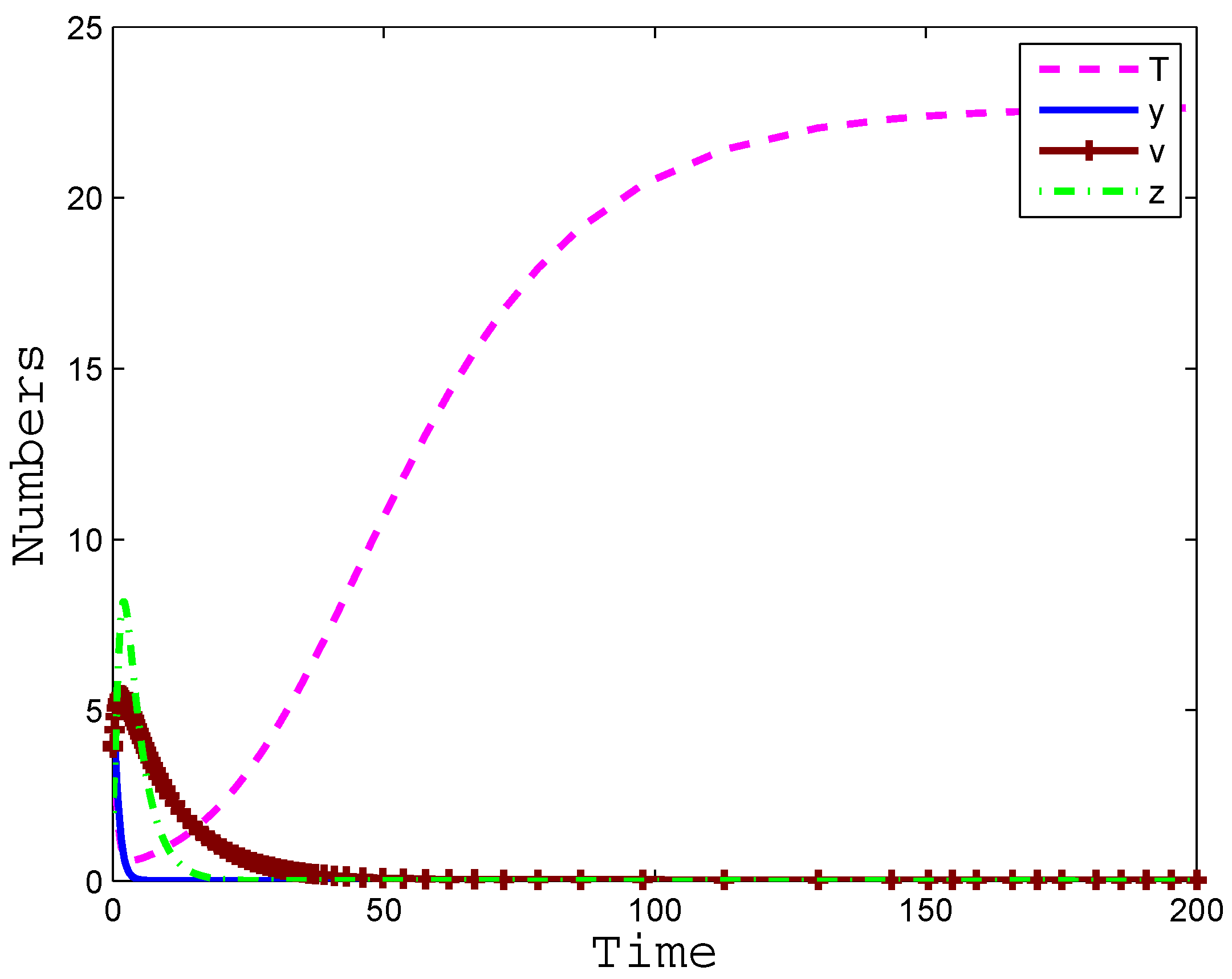
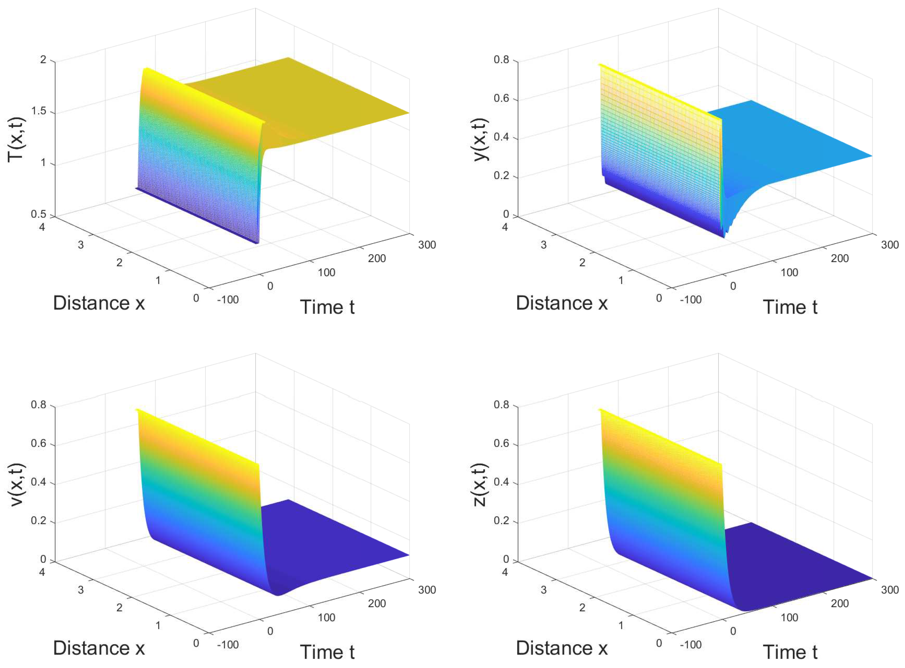
4. Numerical Simulation

In this section, some numerical results of system (4) are presented to support our analytical results. Based on the biological meanings of virus dynamics model from papers [51], we estimated the values of our model parameters as follows:
We first choose T = 5 , I = 2.2 , V = 1.5 , Z = 1.3 . If d 1 = 0 , then the system (4) becomes the following form:
T ( x , t ) t = λ d T ( x , t ) β T ( x , t ) V ( x , t ) , I ( x , t ) t = e a τ β T ( x , t τ ) V ( x , t τ ) a I ( x , t ) p I ( x , t ) Z ( x , t ) , V ( x , t ) t = k I ( x , t ) μ V ( x , t ) , Z ( x , t ) t = c I ( x , t ) Z ( x , t ) b Z ( x , t ) ,
According to the data in Table 1, we first simulate the stability of system (3). If we choose τ = 15 , then we have R 0 < 1 . Therefore, E 0 is globally asymptotically stable. From Figure 1, we can see that except for uninfected cells, the number of the other three populations tends towards zero.
If we choose τ = 6 , then we have R 1 < 1 < R 0 . Hence, C T L -inactivated infection equilibrium E 1 is globally asymptotically stable. From Figure 2, we can see that except for C T L s , the number of the other three populations tends to be certain constants.
If we choose τ = 5 , then we have R 1 > 1 . From Figure 3, we can see that the population of the four compartments of the model are positive constants. Hence, the interior equilibrium E 2 is globally asymptotically stable.
The reproductive ratio plays a crucial role in virus infection dynamics. Actually, in model (4), the basic reproductive ratio R 0 is a decreasing function on time delay τ (see Figure 4a), and the R 1 is also decreasing function on time delay τ (see Figure 4b).
If we choose d 1 = 2 , then we can give a numerical simulation of the stability of system (4). Using the data in Table 1, we can first simulate the stability of the interior equilibrium (see Figure 5).
From Figure 5, we can see that due to the effect of diffusion, the process of population increase and decrease is not stable. The rise and fall of the population is very volatile in a short period of time.
If we choose β = 0.03 , then we have R 0 < 1 . Therefore, E 0 is globally asymptotically stable (see Figure 6).
If we choose k = 0.002 , then we have R 1 < 1 < R 0 . Therefore, E 1 is globally asymptotically stable (see Figure 7).
As in Figure 5, the changes in the number of people in Figure 7 are also fluctuating.

5. Conclusions and Discussion

It is necessary to understand the dynamics model for HIV infection since these infected cells usually cause a C T L response from the immune system. In this paper, we developed a diffusive infection model (4) with the cell-mediated immune response and intracellular delay on the base of the model (3), and the corresponding discrete system. We studied HIV infection dynamics for the purpose of better understanding how the effect of diffusion impacts the process of population. Without other additional conditions, we obtained their basic reproduction number R 0 which plays a crucial role in the proof of our results. By constructing the Lyapunov function, we proved the global stability of the equilibria: the trivial equilibrium of the above model is globally asymptotically stable if R 0 1 ; the C T L -inactivated infection equilibrium is globally asymptotically stable when R 1 1 < R 0 ; the interior equilibrium is globally asymptotically stable when R 1 > 1 . On the other hand, some numerical simulations are presented to support our analytical results. We saw from the simulations in Figure 1 that E 0 is globally asymptotically. From Figure 4, we obtained that the basic reproductive ratio R 0 is a decreasing function on time delay τ , and the R 1 is also a decreasing function on time delay τ . The effect of diffusion on model (4) is that the process of population increase and decrease is violently fluctuating in a short period of time, which we can see in Figure 5. In general, the system of PDEs cannot be solved explicitly, thus we seek numerical ones instead. By using the NSFD scheme, we show that the proposed discrete model can preserve the global stability of equilibria of the corresponding continuous model. Moreover, how do the other diffusive terms (infected cells, uninfected cells) affect the corresponding model? In future work, we will continue to pay attention to this issue.

Author Contributions

Conceptualization, X.L., C.-C.Z. and H.M.S.; writing—original draft preparation, X.L., C.-C.Z., H.M.S. and H.X.; writing—review and editing, X.L., C.-C.Z., H.M.S. and H.X.; funding acquisition, X.L. and H.X. All authors have read and agreed to the published version of the manuscript.

Funding

The authors were supported by the natural science research of Jiangsu Colleges and Universities (18KJB180027), the Science and Technology Foundation of Suqian (S201818) and (Z2021131), China, and the Talent Introduction Research Foundation of Suqian University (106-CK00042/028), National Natural Science Foundation of China: 12161074.

Institutional Review Board Statement

Not applicable.

Informed Consent Statement

Not applicable.

Data Availability Statement

Not applicable.

Acknowledgments

The first author was supported by the natural science research of JiangSu Colleges and Universities (18KJB180027) and the science and technology foundation of Suqian (S201818) and (Z2021131), China.

Conflicts of Interest

The authors declare no conflict of interest.

References

  1. Calleri, F.; Nastasi, G.; Romano, V. Continuous-time stochastic processes for the spread of COVID-19 disease simulated via a Monte Carlo approach and comparison with deterministicmodels. J. Math. Biol. 2021, 83, 34. [Google Scholar] [CrossRef] [PubMed]
  2. Rihan, F.A.; Alsakaji, H.J.; Rajivganthi, C. Stochastic SIRC epidemic model with time-delay for COVID-19. Adv. Differ. Equ. 2020, 2020, 502. [Google Scholar] [CrossRef] [PubMed]
  3. Li, Y. The necessity analysis of the knowledge dissemination of hypertension disease prevention in public english teaching. Indian J. Pathol. Microbiol. 2020, 82, 40. [Google Scholar]
  4. Zeng, Q.; Bie, B.; Guo, Q.; Yuan, Y.; Han, Q.; Han, X.; Chen, M.; Zhang, X.; Yang, Y.; Liu, M.; et al. Hyperpolarized Xe NMR signal advancement by metal-organic framework entrapment in aqueous solution. Proc. Natl. Acad. Sci. USA 2020, 117, 17558–17563. [Google Scholar] [CrossRef]
  5. Arnaout, R.; Nowak, M.; Wodarz, D. HIV-1 dynamics revisited: Biphasic decay by cytotoxic lymphocyte killing. Proc. Roy. Soc. Lond. B 2000, 265, 1347–1354. [Google Scholar] [CrossRef] [Green Version]
  6. Culshaw, R.; Ruan, S.; Spiteri, R. Optimal HIV treatment by maxinising immune response. J. Math. Biol. 2004, 48, 545–562. [Google Scholar] [CrossRef] [Green Version]
  7. Male, D.; Brostoff, J.; Roth, D.; Roitt, I. Immunology, 7th ed.; Elsevier: Amsterdam, The Netherlands, 2006. [Google Scholar]
  8. Nowak, M.; May, R. Vitus Dynamics; Oxford University Press: Oxford, UK, 2000. [Google Scholar]
  9. Wang, K.; Wang, W.; Liu, X. Global stability in a viral infection model with lytic and nonlytic immune response. Comput. Math. Appl. 2006, 51, 1593–1610. [Google Scholar] [CrossRef] [Green Version]
  10. Wodarz, D. Killer Cell Dynamics: Mathematical and Computational Approaches to Immunology; Springer: Berlin/Heidelberg, Germany, 2007. [Google Scholar]
  11. Kirschner, D.E.; Webb, G.; Cloyd, M. Model of HIV-1 disease progression based on virus-induced lymph node homing and homing-induced apotosis of CD4+ lymphocytes. J. AIDS 2000, 24, 352–362. [Google Scholar]
  12. Weber, J.N.; Weiss, R.A. HIV infection: The cellular picture. Sci. Am. 1988, 259, 101–109. [Google Scholar] [CrossRef]
  13. Murray, J.D. Mathematical Biology; Springer: Berlin/Heidelberg, Germany, 2002. [Google Scholar]
  14. Anderson, R.; May, R. Infections Diseases of Humans: Dynamics and Control; Oxford Univ Press: Oxford, UK, 1991. [Google Scholar]
  15. Boer, R.D.; Perelson, A. Target cell limited and immune control models of HIV infection, A comparison. J. Theoret. Biol. 1998, 190, 201–214. [Google Scholar] [CrossRef] [Green Version]
  16. Nowak, M.; Bangham, C. Population dynamics of immune responses to persistent viruses. Proc. Natl. Acad. Sci. USA 1996, 272, 74–79. [Google Scholar]
  17. Zhu, H.; Zou, X. Dynamics of a HIV-1 infection model with cell-mediated immune response and intracellular delay. Discrete Contin. Dyn. Syst. Ser. B 2009, 12, 511–524. [Google Scholar] [CrossRef]
  18. Wang, J.L.; Guan, L.J. Global stability for a HIV-1 infection model with cell-mediated immune response and intrecellular delay. Discrete Contin. Dyn. Syst. Ser. B 2012, 17, 297–302. [Google Scholar]
  19. Srivastava, H.M.; Deniz, S. A new modified semi-analytical technique for a fractional-order Ebola virus disease model. Rev. Real Acad. Cienc. Exactas Fís. Natur. Ser. A Mat. (RACSAM) 2021, 115, 137. [Google Scholar] [CrossRef]
  20. Srivastava, H.M.; Jan, R.; Jan, A.; Deebani, W.; Shutaywi, M. Fractional-calculus analysis of the transmission dynamics of the dengue infection. Chaos 2021, 31, 53130. [Google Scholar] [CrossRef]
  21. Srivastava, H.M.; Saad, K.M.; Gómez-Aguilar, J.F.; Almadiy, A.A. Some new mathematical models of the fractional-order system of human immune against IAV infection. Math. Biosci. Eng. 2020, 17, 4942–4969. [Google Scholar] [CrossRef]
  22. Zhu, C.C.; Zhu, J. Stability of a reaction-diffusion alcohol model with the impact of tax policy. Comput. Math. Appl. 2017, 74, 613–633. [Google Scholar] [CrossRef]
  23. Li, H.C.; Peng, R.; Wang, Z.A. On a Diffusive Susceptible-Infected-Susceptible Epidemic Model with Mass Action Mechanism and Birth-Death Effect: Analysis, Simulations, and Comparison with Other Mechanisms. SIAM J. Appl. Math. 2018, 78, 2129–2153. [Google Scholar] [CrossRef]
  24. Jin, H.Y.; Wang, Z.A. Boundedness, blowup and critical mass phenomenon incompeting chemotaxis. J. Differ. Equ. 2016, 260, 162–196. [Google Scholar] [CrossRef]
  25. Sigdel, R.P.; Mcluskey, C.C. Global stability for an SEI model of infection disease with immigration. Appl. Math. Comput. 2014, 243, 684–689. [Google Scholar]
  26. Srivastava, H.M.; Ahmad, H.; Ahmad, I.; Thounthong, P.; Khan, M.N. Numerical simulation of 3-D fractional-order convection-diffusion PDE by a local meshless method. Thermal. Sci. 2021, 25, 347–358. [Google Scholar] [CrossRef]
  27. Srivastava, H.M.; Izadi, M.; Okhovati, N. Viscous splitting finite difference schemes to convection-diffusion equations with discontinuous coefficient. Appl. Anal. Optim. 2022, 6, 313–328. [Google Scholar]
  28. Srivastava, H.M.; Izadi, M. The Rothe–Newton approach to simulate the variable coefficient convection-diffusion equations. J. Mahani Math. Res. Cent. 2022, 11, 141–157. [Google Scholar]
  29. Xu, H.Y.; Li, H.; Xuan, Z.C. Some new inequalities on Laplace–Stieltjes transforms involving logarithmic growth. Fractal Fract. 2022, 6, 233. [Google Scholar] [CrossRef]
  30. Xu, H.Y.; Xu, L. Transcendental entire solutions for several quadratic binomial and trinomial PDEs with constant coefficients. Anal. Math. Phys. 2022, 12, 64. [Google Scholar] [CrossRef]
  31. Xu, H.Y.; Jiang, Y.y. Results on entire and meromorphic solutions for several systems of quadratic trinomial functional equations with two complex variables, Revista de la Real Academia de Ciencias Exactas, Físicas y Naturales. Ser. A Matemáticas 2022, 116, 1–19. [Google Scholar]
  32. Li, H.; Xu, H.Y. Notes on solutions for some systems of complex functional equations in C2. J. Funct. Spaces 2021, 2021, 5424284. [Google Scholar]
  33. Xu, H.Y.; Kong, Y.Y. Entire functions represented by Laplace-Stieltjes transforms concerning the approximation and generalized order. Acta Math. Sci. 2021, 41, 646–656. [Google Scholar] [CrossRef]
  34. Xu, H.Y.; Liu, S.Y.; Li, Q.P. Entire solutions for several systems of nonlinear difference and partial differential-difference equations of Fermat-type. J. Math. Anal. Appl. 2020, 483, 123641. [Google Scholar] [CrossRef]
  35. Xu, H.Y.; Kong, Y.Y. The approximation of Laplace–Stieltjes transformations with finite order on the left half plane. Comptes Rendus Math. 2018, 356, 63–76. [Google Scholar] [CrossRef]
  36. Liu, X.L.; Zhu, C.C. A Non-Standard Finite Difference Scheme for a Diffusive HIV-1 Infection Model with Immune Response and Intracellular Delay. Axioms. 2022, 11, 129. [Google Scholar] [CrossRef]
  37. Enatsu, Y.; Nakata, Y.; Muroya, Y.; Izzo, G.; Vecchio, A. Global dynamics of difference equations for SIR epidemic models with a class of nonlinear incidence rates. J. Differ. Equ. Appl. 2012, 18, 1163–1181. [Google Scholar] [CrossRef] [Green Version]
  38. Mickens, R.E. Nonstandard Finite Difference Models of Differential Equations; World Scientific: Singapore, 1994. [Google Scholar]
  39. Hattaf, K.; Yousfi, N. Global properties of a discrete viral infection model with general incidence rate. Math. Methods Appl. Sci. 2016, 39, 998–1004. [Google Scholar] [CrossRef]
  40. Shi, P.; Dong, L. Dynamical behaviors of a discrete HIV-1 virus model with bilinear infective rate. Math. Methods Appl. Sci. 2014, 37, 2271–2280. [Google Scholar]
  41. Wang, J.P.; Teng, Z.D.; Miao, H. Global dynamics for discrete-time analog of viral infection model with nonlinear incidence and CTL immune response. Adv. Differ. Equ. 2016, 2016, 143. [Google Scholar] [CrossRef] [PubMed] [Green Version]
  42. Xu, J.H.; Geng, Y. Dynamic consistent NSFD Scheme for a Delayed Viral Infection Model with Immune Response and Nonlinear Incidence. Discret. Nat. Soc. 2017, 2017, 3141736. [Google Scholar] [CrossRef] [Green Version]
  43. Yang, Y.; Zhou, J. Global dynamics of a PDE in-host viral model. Appl. Anal. 2014, 93, 2312–2329. [Google Scholar]
  44. Fitzgibbon, W.E. Semilinear functional differential equations in Banach space. J. Differ. Equ. 1978, 29, 1–14. [Google Scholar] [CrossRef] [Green Version]
  45. Martin, R.H.; Smith, H.L. Abstract functional differential equations and reaction-diffusion systems. Trans. Am. Math. Soc. 1990, 321, 1–44. [Google Scholar]
  46. Martin, R.H.; Smith, H.L. Reaction-diffusion systems with time delays: Monotonicity, invariance, comparison and convergence. J. Reine Angew. Math. 1991, 413, 1–35. [Google Scholar]
  47. Travis, C.C.; Webb, G.F. Existence and stability for partial functional differential equations. Trans. Am. Math. Soc. 1974, 200, 395–418. [Google Scholar] [CrossRef]
  48. Wu, J. Theory and Applications of Parfunctional Differential Equations; Springer: New York, NY, USA, 1996. [Google Scholar]
  49. Protter, M.H.; Weinberger, H.F. Maximum Principles in Differential Equations; Prentice Hall: Engle-Wood Cliffs, NJ, USA, 1967. [Google Scholar]
  50. Henry, D. Gerometric Theory of Semilinear Parabolic Equation; Lecture Notes in Mathematics; Springer: Berlin/Heidelberg, Germany, 1993. [Google Scholar]
  51. Xiang, H.; Tang, Y.L.; Huo, H.F. A viral model with intracellular delay and humoral immunity. Bull. Malays. Math. Sci. Soc. 2016. [Google Scholar] [CrossRef]
  52. Nelson, P.; Murray, J.; Perelson, A. A model of HIV-1 pathogenesis that includes an intracellular delay. Math. Biosci. 2000, 163, 201–215. [Google Scholar] [CrossRef]
Figure 1. When τ = 15 , R 0 < 1 , the infection-free equilibrium E 0 is globally asymptotically stable.
Mathematics 10 04296 g001
Figure 2. When τ = 6 , R 1 < 1 < R 0 , the C T L -inactivated infection equilibrium E 1 is globally asymptotically stable.
Mathematics 10 04296 g002
Figure 3. When τ = 5 , R 1 > 1 , the interior equilibrium E 2 is globally asymptotically stable.
Mathematics 10 04296 g003
Figure 4. (a): R 0 is a decreasing function on time delay τ , (b): R 1 is a decreasing function on time delay τ .
Mathematics 10 04296 g004
Figure 5. When d 1 = 2 , R 1 > 1 , the interior equilibrium E 2 is globally asymptotically stable.
Mathematics 10 04296 g005
Figure 6. When d 1 = 2 , R 0 < 1 , the infection-free equilibrium E 0 is globally asymptotically stable.
Mathematics 10 04296 g006
Figure 7. When d 1 = 2 , R 1 < 1 < R 0 , the infection-free equilibrium E 1 is globally asymptotically stable.
Mathematics 10 04296 g007
Table 1. State variables and parameters of HIV-1 infection model.
ParameterDescription
λ 0.9 day 1 Reference [51]
d0.03 day 1 Reference [52]
β 0.3 day 1 Reference [51]
μ 0.1 day 1 Reference [51]
a0.5 year 1 Reference [52]
b0.3 day 1 Reference [51]
k0.5 day 1 Reference [51]
p0.08Estimate
c0.4 day 1 Estimate
Publisher’s Note: MDPI stays neutral with regard to jurisdictional claims in published maps and institutional affiliations.

