
Joint Optimization of Multi-Cycle Timetable Considering Supply-to-Demand Relationship and Energy Consumption for Rail Express
Abstract
:1. Introduction
1.1. Background
1.2. Literature Reviews
1.3. Potential Contributions
- A periodized spatial-temporal network that can support the integrated optimization of passenger service satisfaction and energy consumption is studied. To describe the acceleration and deceleration behavior of trains due to stopping, a vertex set and an arc set of the spatial-temporal network are created based on the decomposed actions of the trains’ movements. The network can be used to determine the spatial-temporal path of trains, which in turn enables the integrated optimization of passenger service satisfaction and energy consumption.
- An integrated optimization model taking the train spatial-temporal path, cycle length and active lines as the variables is proposed. The objective function composes the supply–demand matching degree (SDMD), the minimum time cost (MTC) and the energy consumption (EC), where the SDMD is measured by the difference between the demand flow and train frequency in each time duration, and the MTC and EC are measured by the costs of the spatial-temporal paths. Four classes of constraints are considered, including the train flow balance constraints, cycle interval constraints, incompatible constraints and minimum travel time constraints.
- A hybrid heuristic Lagrangian decomposition method is proposed. The determination of the cycle length and line and the scheduling of the spatial-temporal points in the train diagram are separated, where the scheduling of the train diagram is further decomposed into an independent problem by the Lagrangian relaxation.
2. Methodology
- The supply–demand matching set in this paper focuses on the supply–demand matching of several stations. We believe that the trains’ transportation capacity in a line needs to be prioritized to satisfy the stations with larger passenger flows, and other stations with smaller passenger flows can be appropriately ignored. Therefore, the set of stations to be concerned and their corresponding passenger flows will be given in the modeling process of this paper. This assumption is in line with the planning convention in actual transportation organization.
- The numbers of passengers on board in each station are preset as an input for the model. In the course of practical application, the specific OD volume and dynamic upload and download of passenger flow is difficult to count. We pre-estimate the numbers of passenger that can be served in each station by means of passenger ticket allocation techniques.
- The time resolution of the spatial-temporal network is set to 1 min.
2.1. Notations and Modeling Basis
2.2. Augmented Spatial-Temporal Network for Multi-Cycle Timetabiling
2.2.1. Spatial-Temporal Vertexes for Augmented Spatial-Temporal Network
2.2.2. Arc Set Considering Differences in Energy Consumption for Various Train Behaviors
2.3. Optimization Model for Scheduling MTSDE
2.3.1. Objective Function
2.3.2. Constraint Condition
2.3.3. Sets of Incompatible Arcs
2.4. Decomposition Algorithm Based on Hybrid Heuristic Lagrangian Relaxation (HHLR)
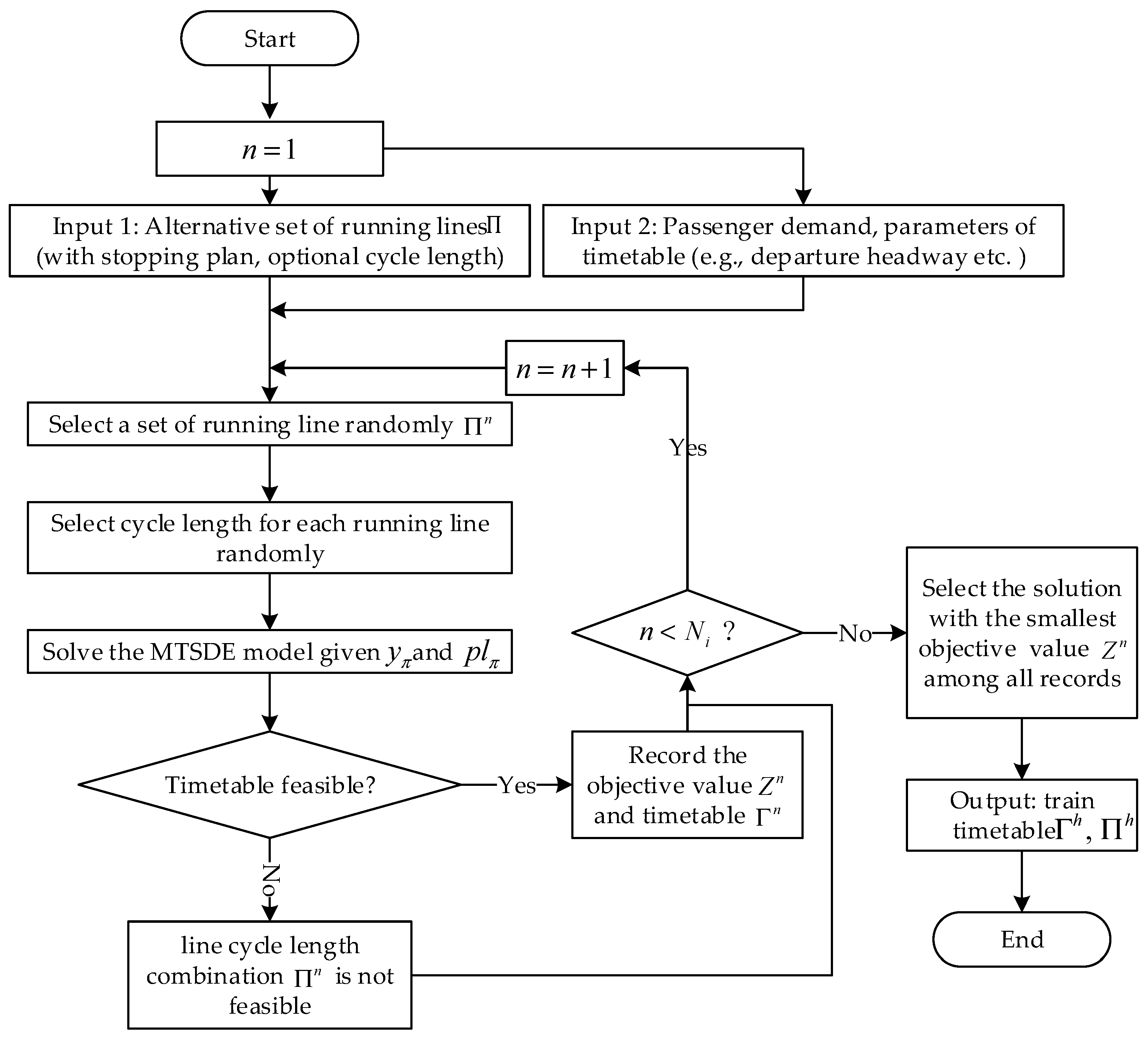
2.4.1. Optional Set-Based Algorithm Framework
2.4.2. Decomposition of the Original MTSDE Model
| Algorithm 1 Lagrangian Decomposition Algorithm | |
| 1: | Lagrangian Relaxation: According to the Lagrange relaxation of the original integer programming problem , the corresponding relaxation problem is obtained. |
| 2: | Problem decomposition: Relaxation problem is decomposed into about independent of the shortest path problem . |
| 3: | Initialize: In order to solve the train schedule problem , let the initial iteration number , the corresponding Lagrange multiplier , the upper bound objective function value is , and the lower bound objective function value is |
| 4: | while or then |
| 5: | According to the current Lagrange multiplier, the problem with constraints is solved using dynamics programming algorithm and obtains the lower bound solution . |
| 6: | Calculate the objective function value of problem corresponding to the lower bound solution . |
| 7: | if then |
| 8: | Update the optimal lower bound solution, let . |
| 9: | end if |
| 10: | The upper bound solution is obtained by using the greedy algorithm for . |
| 11: | Compute the objective function value of the problem corresponding to the upper bound solution |
| 12: | if then |
| 13: | Update the optimal upper bound solution, let |
| 14: | end if |
| 15: | Lagrange multipliers are updated by sub gradient method. |
| 16: | |
| 17: | |
| 18: | end while |
| 19: | return |
2.4.3. Lower Bound Solution Algorithm of Lagrangian Sub-Problem Based on Dynamic Programming Algorithm
2.4.4. Upper Bound Solution of Lagrangian Sub-Problem Based on Heuristic Algorithm
| Algorithm 2 Greedy Algorithm | |
| 1: | According to the results of the lower bound solution, the optimal objective values of the sub-problem s are sorted from small to large so that the train with the smallest optimal objective is ranked first |
| 2: | The train’s spatial-temporal path is arranged one by one, according to the sequence order, by solving the shortest path |
| 3: | Search all feasible paths to find the shortest path of the train. The network does not contain any arc that is incompatible with the arc passed by the last train by eliminating arcs who violate the arrival headway, departure headway constraints, etc. |
| 4: | Output: a set of values of all 𝑘∈𝐾, and 𝑢→𝑣∈𝐴, obtain all train paths. |
2.4.5. The Updates of Lagrangian Multipliers
3. Numerical Experiments
3.1. Experiment Designs
3.2. Comparison of Single-Cycle and Multi-Cycle Train Timetable under Different Scenarios
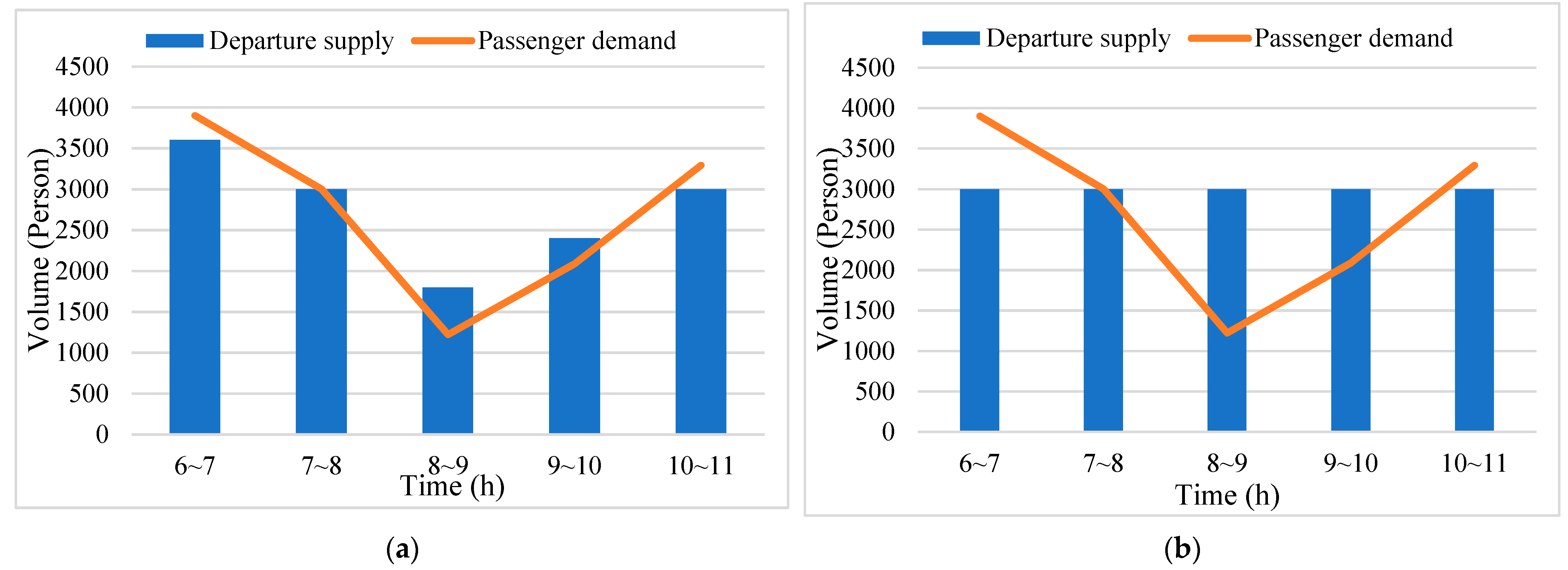
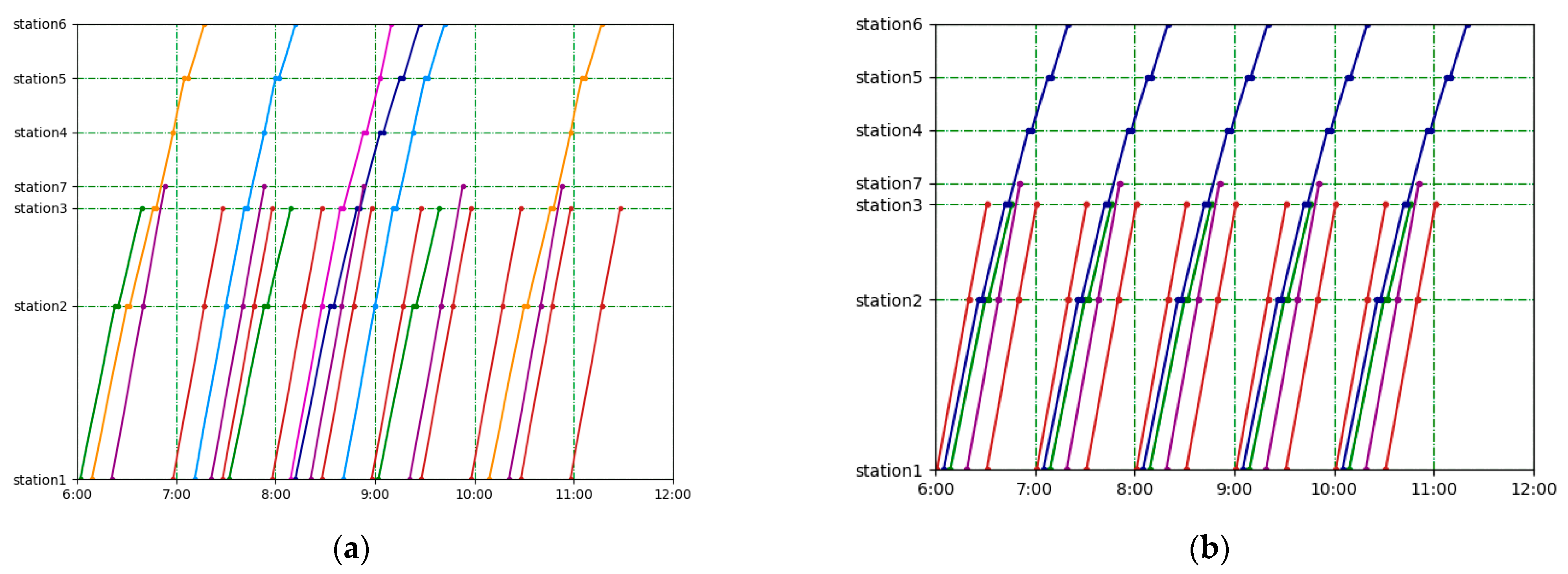
3.2.1. Scenario 1 with Two Passenger Flow Peaks
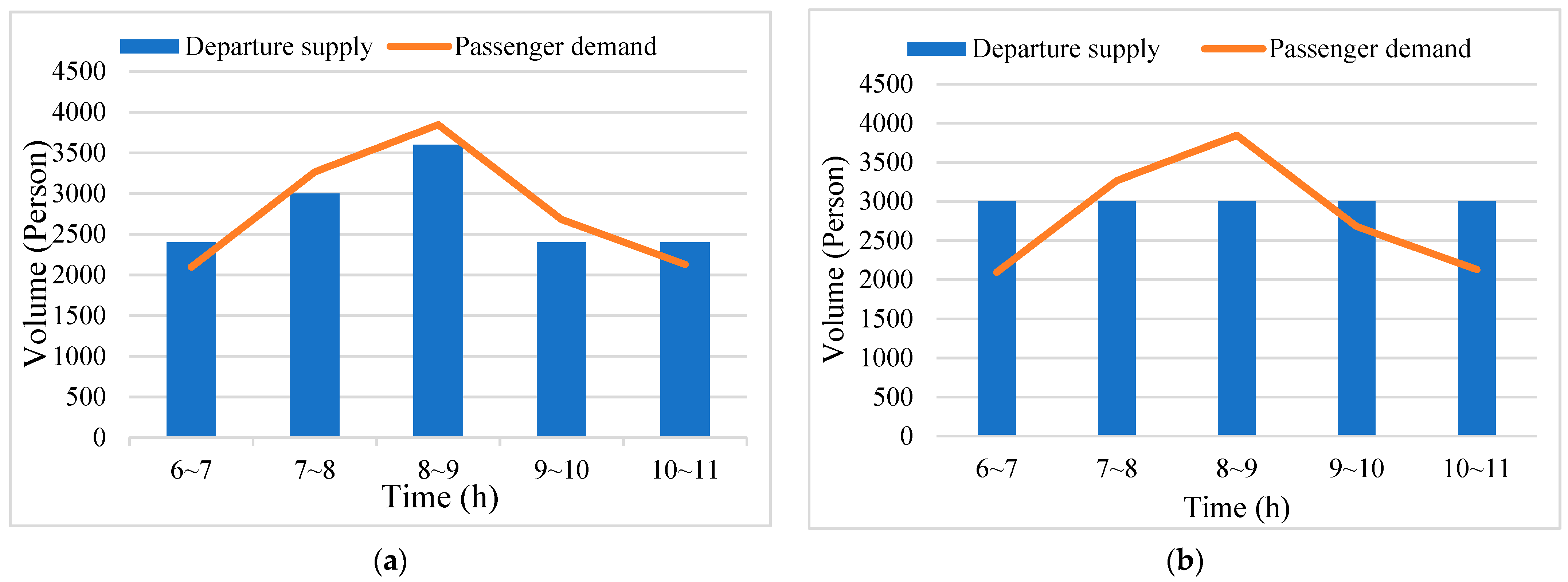
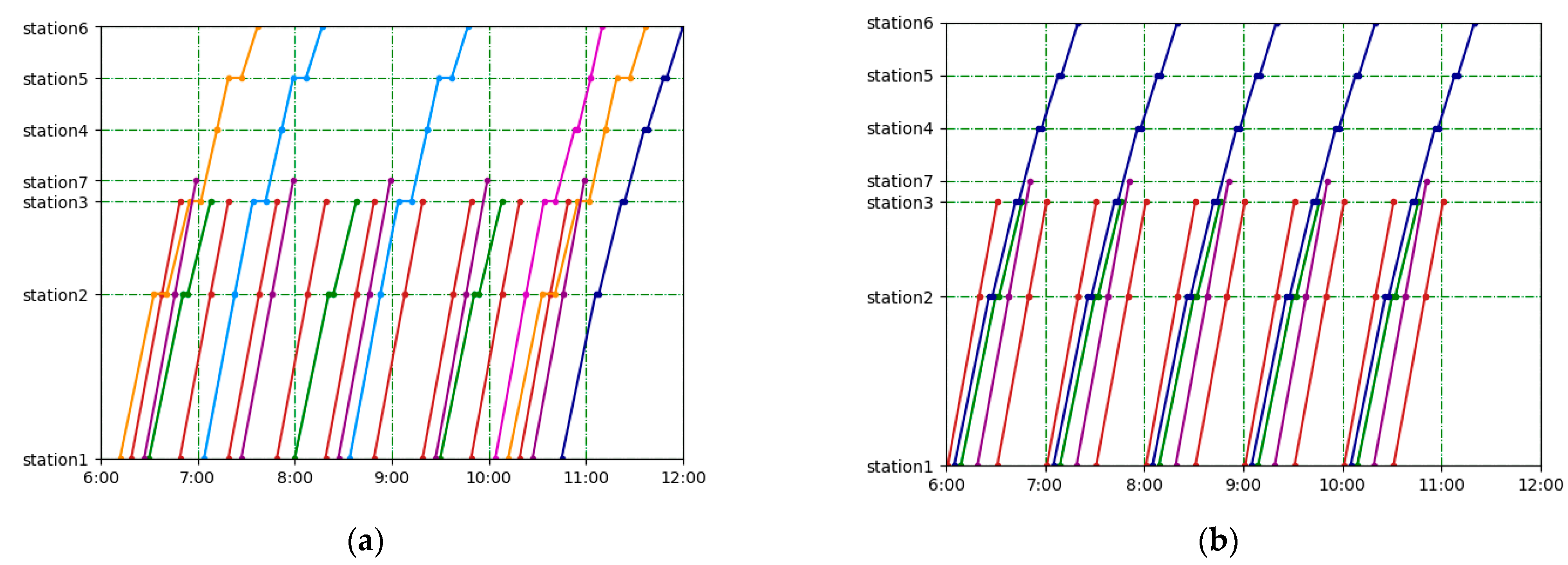
3.2.2. Scenario 2 with One Passenger Flow Peaks
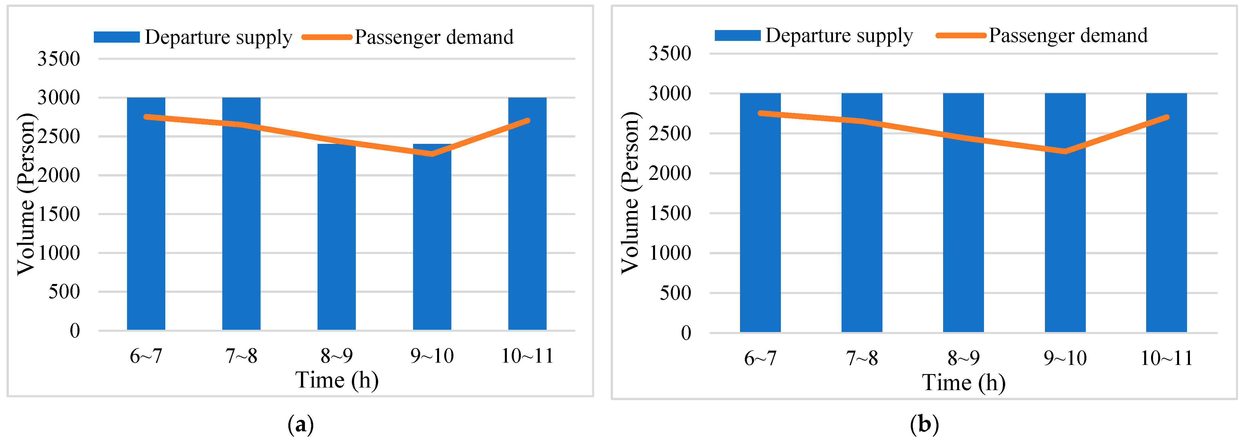
3.2.3. Scenario 3 without Passenger Flow Peaks
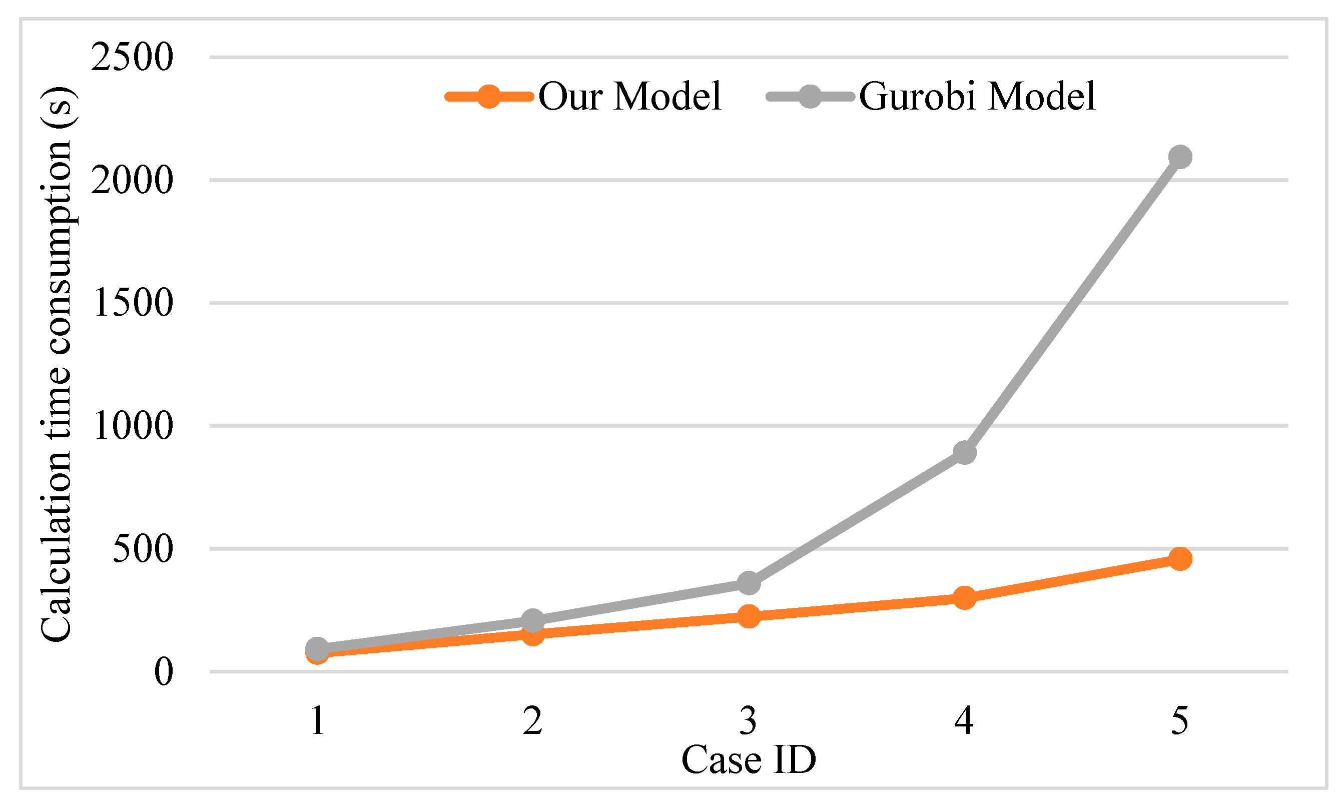
3.3. Analysis of Solution Efficiency
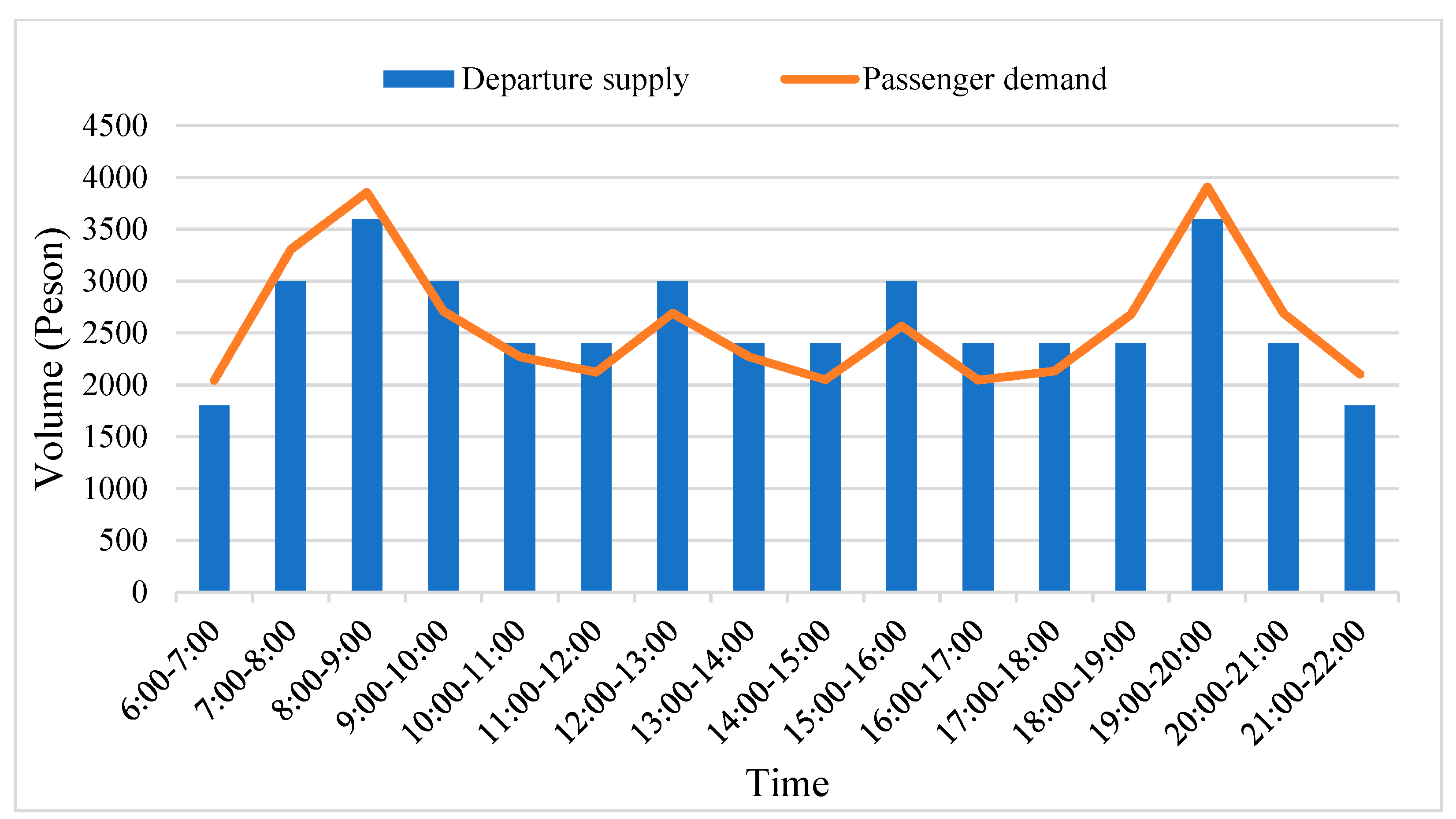
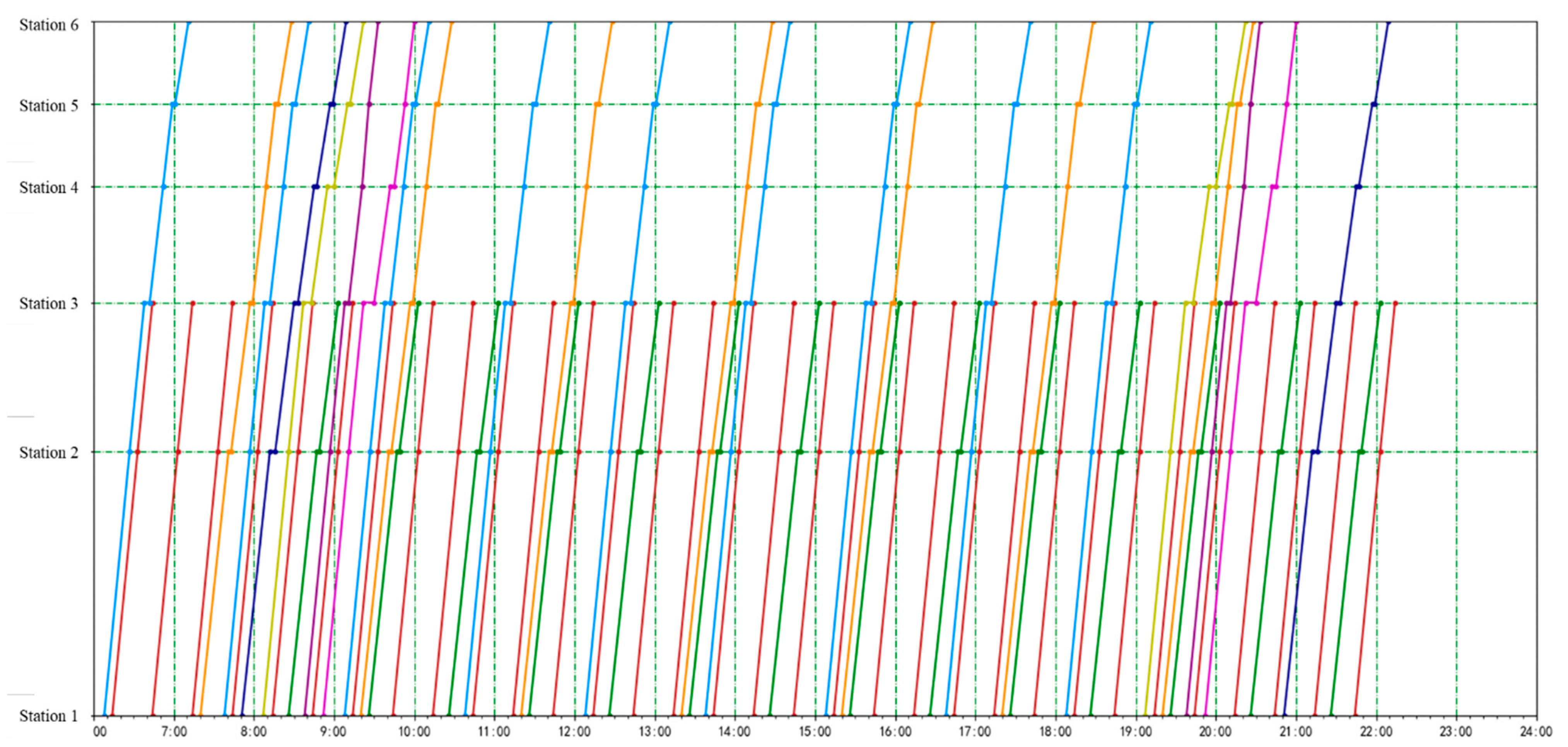
3.4. Experiment Based on Real-World Case
3.5. Discussion
4. Conclusions
Author Contributions
Funding
Data Availability Statement
Conflicts of Interest
Abbreviations
| Abbreviation | Description |
| PESP | Periodic event scheduling problem |
| OD | Origin–destination |
| MTSDE | Multi-cycle timetable considering supply-to-demand relationship and energy consumption |
| SDMD | Supply–demand matching degree |
| MTC | Minimum time cost |
| EC | Energy consumption |
| HHLR | Hybrid heuristic Lagrangian relaxation |
| LB | Lower bound |
| UB | Upper bound |
| MT | Multi-cycle train timetable |
| ST | Single-cycle train timetable |
References
- Wang, B.; Yang, H.; Zhang, Z.H. Research on the train operation plan of the beijing-tianjin inter-city railway based on periodic train diagrams. Tiedao Xuebao/J. China Railw. Soc. 2007, 29, 8–13. [Google Scholar]
- Serafini, P.; Ukovich, W. A mathematical model for periodic scheduling problems. SIAM J. Discret. Math. 1989, 2, 550–581. [Google Scholar] [CrossRef]
- Peeters, L.W.P. Cyclic Railway Timetable Optimization; Erasmus University Rotterdam: Rotterdam, The Netherlands, 2003. [Google Scholar]
- Cordone, R.; Redaelli, F. Optimizing the demand captured by a railway system with a regular timetable. Transp. Res. Part B Methodol. 2011, 45, 430–446. [Google Scholar] [CrossRef]
- Goerigk, M.; Schöbel, A. Improving the modulo simplex algorithm for large-scale periodic timetabling. Comput. Oper. Res. 2013, 40, 1363–1370. [Google Scholar] [CrossRef]
- Zhang, X.; Nie, L. Integrating capacity analysis with high-speed railway timetabling: A minimum cycle time calculation model with flexible overtaking constraints and intelligent enumeration. Transp. Res. Part C Emerg. Technol. 2016, 68, 509–531. [Google Scholar] [CrossRef]
- Herrigel, S.; Laumanns, M.; Szabo, J.; Weidmann, U. Periodic railway timetabling with sequential decomposition in the pesp model. J. Rail Transp. Plan. Manag. 2018, 8, 167–183. [Google Scholar] [CrossRef]
- Kinder, M. Models for Periodic Timetabling. Master’s Thesis, Technische Universität Berlin, Berlin, Germany, 2008. [Google Scholar]
- Caprara, A.; Fischetti, M.; Toth, P. Modeling and solving the train timetabling problem. Oper. Res. 2002, 50, 851–861. [Google Scholar] [CrossRef]
- Zhang, Y.; Peng, Q.; Yao, Y.; Zhang, X.; Zhou, X. Solving cyclic train timetabling problem through model reformulation: Extended time-space network construct and alternating direction method of multipliers methods. Transp. Res. Part B Methodol. 2019, 128, 344–379. [Google Scholar] [CrossRef]
- Odijk, M.A. A constraint generation algorithm for the construction of periodic railway timetables. Transp. Res. Part B Methodol. 1996, 30, 455–464. [Google Scholar] [CrossRef]
- Robenek, T.; Sharif Azadeh, S.; Maknoon, Y.; Bierlaire, M. Hybrid cyclicity: Combining the benefits of cyclic and non-cyclic timetables. Transp. Res. Part C Emerg. Technol. 2017, 75, 228–253. [Google Scholar] [CrossRef] [Green Version]
- Zhou, W.; Yang, X. Timetable optimization for high-speed rail with multiple operating periods: Solving method based on a framework of lagrangian relaxation decomposition. Transp. Res. Rec. 2016, 2546, 43–52. [Google Scholar] [CrossRef]
- Zhou, W.; Tian, J.; Xue, L.; Jiang, M.; Deng, L.; Qin, J. Multi-periodic train timetabling using a period-type-based lagrangian relaxation decomposition. Transp. Res. Part B Methodol. 2017, 105, 144–173. [Google Scholar] [CrossRef]
- Yan, F.; Goverde, R.M.P. Combined line planning and train timetabling for strongly heterogeneous railway lines with direct connections. Transp. Res. Part B Methodol. 2019, 127, 20–46. [Google Scholar] [CrossRef]
- Niu, H.; Zhou, X.; Gao, R. Train scheduling for minimizing passenger waiting time with time-dependent demand and skip-stop patterns: Nonlinear integer programming models with linear constraints. Transp. Res. Part B Methodol. 2015, 76, 117–135. [Google Scholar] [CrossRef]
- Nachtigall, K.; Voget, S. A genetic algorithm approach to periodic railway synchronization. Comput. Oper. Res. 1996, 23, 453–463. [Google Scholar] [CrossRef]
- Liebchen, C. The first optimized railway timetable in practice. Transp. Sci. 2008, 42, 420–435. [Google Scholar] [CrossRef]
- Cordeau, J.-F.; Toth, P.; Vigo, D. A survey of optimization models for train routing and scheduling. Transp. Sci. 1998, 32, 380–404. [Google Scholar] [CrossRef]
- Yin, Y.; Li, D.; Bešinović, N.; Cao, Z. Hybrid demand-driven and cyclic timetabling considering rolling stock circulation for a bidirectional railway line. Comput.-Aided Civ. Infrastruct. Eng. 2019, 34, 164–187. [Google Scholar] [CrossRef]
- Kim, N.s.; Van Wee, B.J.T.P. Assessment of CO2 emissions for truck-only and rail-based intermodal freight systems in europe. Transp. Plan. Technol. 2009, 32, 313–333. [Google Scholar] [CrossRef]
- Ritzinger, U.; Puchinger, J.; Hartl, R.F. Dynamic programming based metaheuristics for the dial-a-ride problem. Ann. Oper. Res. 2016, 236, 341–358. [Google Scholar] [CrossRef] [Green Version]
- Jørgensen, M.W.; Sorenson, S.C. Estimating Emissions from Railway Traffic; Technical University of Denmark: Lyngby, Denmark, 1998; Volume 20, pp. 210–218. [Google Scholar]
- Kirschstein, T.; Meisel, F. Ghg-emission models for assessing the eco-friendliness of road and rail freight transports. Transp. Res. Part B Methodol. 2015, 73, 13–33. [Google Scholar] [CrossRef]
- Zhou, X.; Tanvir, S.; Lei, H.; Taylor, J.; Liu, B.; Rouphail, N.M.; Christopher Frey, H. Integrating a simplified emission estimation model and mesoscopic dynamic traffic simulator to efficiently evaluate emission impacts of traffic management strategies. Transp. Res. Part D Transp. Environ. 2015, 37, 123–136. [Google Scholar] [CrossRef]
- Lindgreen, E.B.G.; Sorenson, S.C. Simulation of Energy Consumption and Emissions from Rail Traffic; Technical University of Denmark: Lyngby, Denmark, 2005. [Google Scholar]
- Patterson, Z.; Ewing, G.O.; Haider, M. The potential for premium-intermodal services to reduce freight co2 emissions in the quebec city–windsor corridor. Transp. Res. Part D Transp. Environ. 2008, 13, 1–9. [Google Scholar] [CrossRef]
- Lukaszewicz, P. Energy saving driving methods for freight trains. In Proceedings of the International Conference on Computer Aided Design, San Jose, CA, USA, 7–11 November 2004. [Google Scholar]
- Cortés, C.E.; Vargas, L.S.; Corvalán, R.M. A simulation platform for computing energy consumption and emissions in transportation networks. Transp. Res. Part D Transp. Environ. 2008, 13, 413–427. [Google Scholar] [CrossRef]
- Heinold, A.; Meisel, F. Emission rates of intermodal rail/road and road-only transportation in europe: A comprehensive simulation study. Transp. Res. Part D Transp. Environ. 2018, 65, 421–437. [Google Scholar] [CrossRef]
- Wu, Q.; Spiryagin, M.; Cole, C. Train energy simulation with locomotive adhesion model. Railw. Eng. Sci. 2020, 28, 75–84. [Google Scholar] [CrossRef] [Green Version]
- Chen, D.; Li, S.; Li, J.; Ni, S.; Liu, X. Optimal high-speed railway timetable by stop schedule adjustment for energy-saving. J. Adv. Transp. 2019, 2019, 4213095. [Google Scholar] [CrossRef]
- Zhang, H.; Jia, L.; Wang, L.; Xu, X. Energy consumption optimization of train operation for railway systems: Algorithm development and real-world case study. J. Clean. Prod. 2019, 214, 1024–1037. [Google Scholar] [CrossRef]
- Albrecht, T.; Oettich, S. A new integrated approach to dynamic schedule synchronization and energy-saving train control. Comput. Railw. VIII 2002, 61, 847–856. [Google Scholar]
- Li, X.; Lo, H.K. Energy minimization in dynamic train scheduling and control for metro rail operations. Transp. Res. Part B Methodol. 2014, 70, 269–284. [Google Scholar] [CrossRef]
- Lancien, D.; Fontaine, M. Computing train schedules to save energy: The mareco program. Revue Generale Des Chemins De Fer. 1981, 100, 679–692. [Google Scholar]
- Bai, Y.; Mao, B.; Zhou, F.; Ding, Y.; Dong, C. Energy-efficient driving strategy for freight trains based on power consumption analysis. J. Transp. Syst. Eng. Inf. Technol. 2009, 9, 43–50. [Google Scholar] [CrossRef]
- Burggraeve, S.; Bull, S.H.; Vansteenwegen, P.; Lusby, R.M. Integrating robust timetabling in line plan optimization for railway systems. Transp. Res. Part C Emerg. Technol. 2017, 77, 134–160. [Google Scholar] [CrossRef]
- Mahmoudi, M.; Zhou, X. Finding optimal solutions for vehicle routing problem with pickup and delivery services with time windows: A dynamic programming approach based on state–space–time network representations. Transp. Res. Part B Methodol. 2016, 89, 19–42. [Google Scholar] [CrossRef] [Green Version]
- Camerini, P.M.; Fratta, L.; Maffioli, F. On improving relaxation methods by modified gradient techniques. In Nondifferentiable Optimization; Springer: New York, NY, USA, 1975; pp. 26–34. [Google Scholar]
- Xu, X.; Li, C.-L.; Xu, Z. Integrated train timetabling and locomotive assignment. Transp. Res. Part B Methodol. 2018, 117, 573–593. [Google Scholar] [CrossRef]


| Type | Notation | Definition |
|---|---|---|
| Set | Set of trains | |
| Set of line plan , where is the element of line plan | ||
| Origin station index of line | ||
| Destination station index of line | ||
| Set of stations | ||
| Set of stations along line ’s route | ||
| Set of no-skip stations along line ’s route | ||
| Set of trains belonging to a line , where Kπ ⊂ K, | ||
| The number of time durations used for calculating passenger demand satisfaction. , where is the number of time duration. These time durations are divided from the whole-time horizon . | ||
| Stations, whose degree of passenger satisfaction needs to be optimized. Generally speaking, it is the stations in the line with high passenger flow. | ||
| Parameter | Minimum arrival headway of station | |
| Minimum departure headway of station | ||
| Number of side tracks in station si ∈ S. If the station has overtravel conditions , otherwise. | ||
| Number of main tracks in station | ||
| The unit cost for train stopping in a station | ||
| The earliest allowed start time of train for running | ||
| The latest allowed end time of train for running | ||
| The pure running time for train to traverse section | ||
| Additional time for train k caused by acceleration | ||
| Additional time for train k caused by deceleration | ||
| The minimum required dwell time of train at station | ||
| Operating cost unit time for train 𝑘 to run | ||
| The departure frequency of the line in the time range T | ||
| Index of the first train in a line | ||
| The order of train in line | ||
| The time interval between two consecutive trains in the same line | ||
| Numbers of passengers that can be served in station i by a train in line planning . If , then , else . | ||
| Passenger demand at station at time | ||
| Start time of the mth time duration, | ||
| The end time of the mth time duration, | ||
| Coefficient of dwelling or waiting energy consumption per time of train | ||
| Coefficient of running energy consumption per time of train ’s departure–arrival arcs | ||
| Coefficient of running energy consumption per time of train ’s departure–passing arcs | ||
| Coefficient of running energy consumption per time of train ’s passing–arrival arcs | ||
| Coefficient of running energy consumption per time of train ’s passing–passing arcs | ||
| Time cost of arcs of train | ||
| Energy cost of arcs of train | ||
| Variable | If the train of line is passing through arc , then , else | |
| Cycle length of line | ||
| If line is chosen, then , else |
| ID | Name | Notation | Time Cost and Energy Cost of Arcs | Set |
|---|---|---|---|---|
| 1 | Train starting arcs | , , and , then the time cost of arc is ; else | ||
| 2 | Train ending arcs | , , and , then the time cost of arc is ; else ; | ||
| 3 | Train dwelling arcs | , if and , then the time cost of arc is , else . In addition, the energy cost of this arc is . is the coefficient of dwelling or waiting energy consumption per time of train . where . | ||
| 4 | Train waiting arcs | , , and , pk ≤ t ≤ qk − 1, is , . In addition, the energy cost of this arc is . where | ||
| 5 | Train departure arcs | , , and , then the time cost of arc is , . is . where | ||
| 6 | Train departure–arrival arcs in section | , , and , , and , then the time cost of arc is , . In addition, the energy cost of this arc is . is the coefficient of running energy consumption per time of train . | ||
| 7 | Train departure– passing arcs in section | , , and , , , , is , . In addition, the energy cost of this arc is . | ||
| 8 | Train passing–arrival arcs in section | , , and , , , , then the time cost of arc is , . In addition, the energy cost of this arc is . | ||
| 9 | Train passing– passing arcs in section | , , if and , , , , then the time cost of arc is , else . In addition, the energy cost of this arc is where | ||
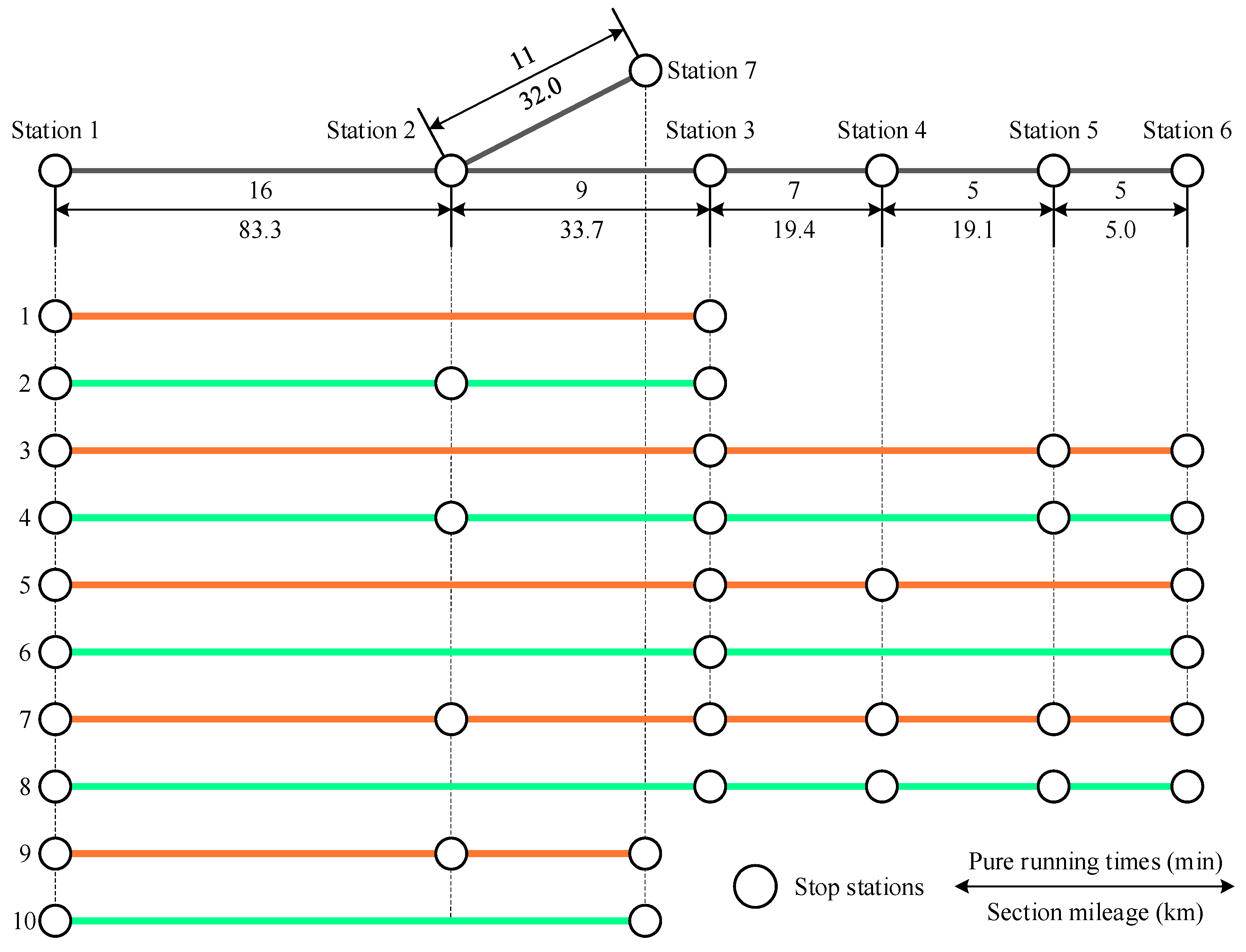
| Line | Origin | Destination | Route | Stop Plans (Intermediate Stations) | Optional Cycle |
|---|---|---|---|---|---|
| 1 | 1 | 3 | 1→2→3 | - | 30, 40 |
| 2 | 1 | 3 | 1→2→3 | 2 | 30, 40, 60, 90 |
| 3 | 1 | 6 | 1→2→3→4→5→6 | 3, 5 | 30, 40, 60, 90 |
| 4 | 1 | 6 | 1→2→3→4→5→6 | 2, 3, 5 | 60, 90, 120, 150, 180 |
| 5 | 1 | 6 | 1→2→3→4→5→6 | 3, 4 | 60, 90, 120, 150, 180, 240, 300, 360, 420, 480, 540, 600, 660, 720, 780, 840, 900, 960 |
| 6 | 1 | 6 | 1→2→3→4→5→6 | 3 | 60, 90, 120, 150, 180, 240, 300, 360, 420, 480, 540, 600, 660, 720, 780, 840, 900, 960, 1020 |
| 7 | 1 | 6 | 1→2→3→4→5→6 | 2, 3, 4, 5 | 60, 90, 120, 150, 180, 240, 300, 360, 420, 480, 540, 600, 660, 720, 780, 840, 900, 960 |
| 8 | 1 | 6 | 1→2→3→4→5→6 | 3, 4, 5 | 60, 90, 120, 150, 180, 240, 300, 360, 420, 480, 540, 600, 660, 720, 780, 840, 900, 960, 1020 |
| 9 | 1 | 7 | 1→2→7 | 2 | 60, 90, 120, 150, 180, 240, 300, 360, 420, 480, 540, 600, 660, 720, 780, 840, 900, 960, 1020 |
| 10 | 1 | 7 | 1→2→7 | - | 30, 40, 50 |
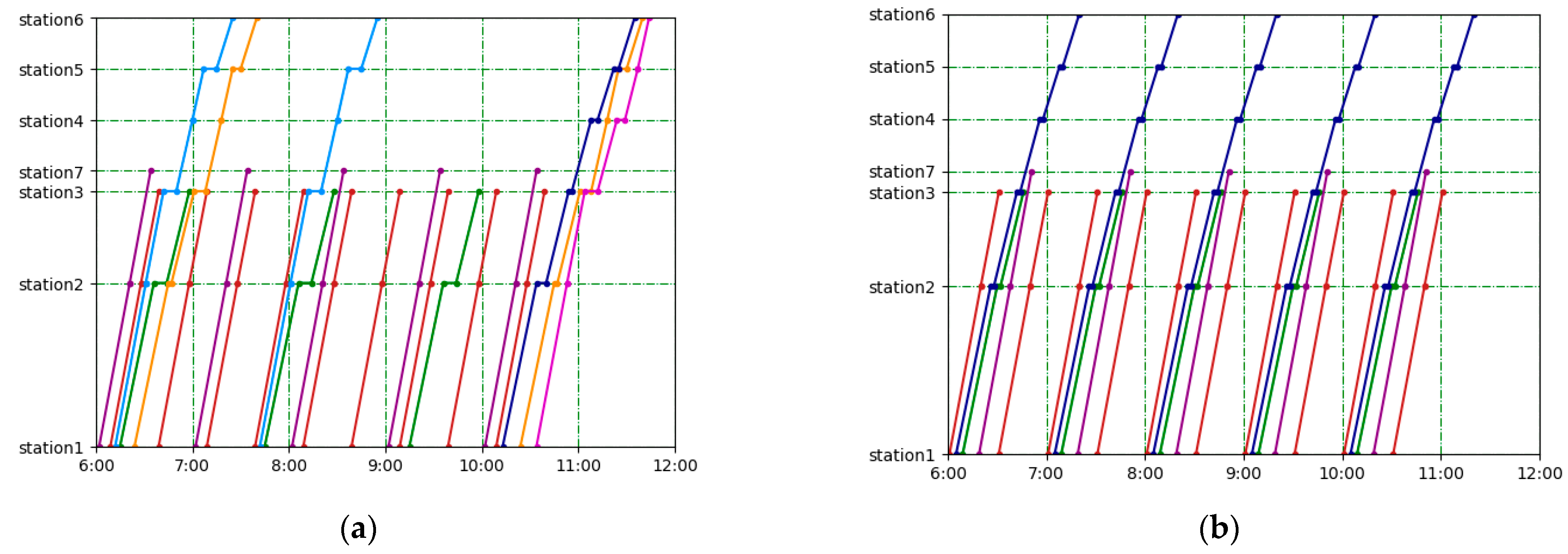
| Figure 4a | 6~7 | 7~8 | 8~9 | 9~10 | 10~11 |
|---|---|---|---|---|---|
| Departure supply | 3600 | 3000 | 1800 | 2400 | 3000 |
| Passenger demand | 3901 | 3001 | 1223 | 2088 | 3293 |
| SDMD * | 92.57% | 99.97% | 62.39% | 86.12% | 91.49% |
| Figure 4b | 6~7 | 7~8 | 8~9 | 9~10 | 10~11 |
|---|---|---|---|---|---|
| Departure supply | 3000 | 3000 | 3000 | 3000 | 3000 |
| Passenger demand | 3901 | 3001 | 1223 | 2088 | 3293 |
| SDMD * | 79.38% | 99.97% | 23.39% | 64.61% | 91.49% |
| Line (Line Color) | |||||||
|---|---|---|---|---|---|---|---|
| 1 (Red) | 2 (Green) | 3 (Blue) | 4 (Orange) | 5 (Violet) | 7 (Navy blue) | 10 (Purple) | |
| MT * | 59,168.79 | 23,362.32 | 26,286.6 | 28,712.86 | 13,143.3 | 16,300.63 | 35,308.45 |
| ST | 65,743.1 | 38,937.2 | 77,847.8 | - | - | - | 35,308.45 |
| Total Number of Trains Running | The Number of Passenger Demand | Demand Satisfaction Ratio | Train Vacancy Rate | Running Time (h) | Energy Consumption (kwh) | |
|---|---|---|---|---|---|---|
| MT * | 25 | 12,911 | 95.59% | 6.44% | 14.33 | 202,282.95 |
| ST | 25 | 12,311 | 91.15% | 17.93% | 17.57 | 217,836.55 |
| Figure 6a | 6~7 | 7~8 | 8~9 | 9~10 | 10~11 |
|---|---|---|---|---|---|
| Departure supply | 2400 | 3000 | 3600 | 2400 | 2400 |
| Passenger demand | 2097 | 3266 | 3845 | 2680 | 2130 |
| SDMD * | 86.55% | 92.18% | 93.83% | 90.08% | 88.09% |
| Figure 6b | 6~7 | 7~8 | 8~9 | 9~10 | 10~11 |
|---|---|---|---|---|---|
| Departure supply | 3000 | 3000 | 3000 | 3000 | 3000 |
| Passenger demand | 2097 | 3266 | 3845 | 2680 | 2130 |
| SDMD * | 65.01% | 92.18% | 80.27% | 88.75% | 66.47% |
| Line (Line Color) | |||||||
|---|---|---|---|---|---|---|---|
| 1 (Red) | 2 (Green) | 3 (Blue) | 4 (Orange) | 5 (Violet) | 7 (Navy blue) | 10 (Purple) | |
| MT * | 59,168.79 | - | 26,286.6 | 28,712.86 | 13,143.3 | 15,569.56 | 35,308.45 |
| ST | 65,743.1 | 38,937.2 | 77,847.8 | - | - | - | 35,308.45 |
| Total Number of Trains Running | The Number of Passenger Demand | Demand Satisfaction Ratio | Train Vacancy Rate | Running Time (h) | Energy Consumption (kwh) | |
|---|---|---|---|---|---|---|
| MT * | 25 | 13,227 | 94.36% | 4.15% | 14.63 | 201,551.88 |
| ST | 25 | 14,618 | 92.07% | 13.95% | 16.95 | 217,836.55 |
| Figure 8a | 6~7 | 7~8 | 8~9 | 9~10 | 10~11 |
|---|---|---|---|---|---|
| Departure supply | 3000 | 3000 | 2400 | 2400 | 3000 |
| Passenger demand | 2753 | 2651 | 2443 | 2273 | 2704 |
| SDMD * | 91.42% | 87.66% | 98.26% | 94.57% | 89.63% |
| Figure 8b | 6~7 | 7~8 | 8~9 | 9~10 | 10~11 |
|---|---|---|---|---|---|
| Departure supply | 3000 | 3000 | 3000 | 3000 | 3000 |
| Passenger demand | 2753 | 2651 | 2443 | 2273 | 2704 |
| SDMD * | 91.42% | 87.66% | 79.61% | 72.63% | 89.63% |
| Line (Line Color) | |||||||
|---|---|---|---|---|---|---|---|
| 1 (Red) | 2 (Green) | 3 (Blue) | 4 (Orange) | 5 (Violet) | 7 (Navy blue) | 10 (Purple) | |
| MT * | 59,168.79 | 23,362.32 | 28,214.84 | 29,676.98 | 13,143.3 | 15,569.56 | 35,308.45 |
| ST | 65,743.1 | 38,937.2 | 77,847.8 | - | - | - | 35,308.45 |
| Total Number of Trains Running | The Number of Passenger Demand | Demand Satisfaction Ratio | Train Vacancy Rate | Running Time (h) | Energy Consumption (kwh) | |
|---|---|---|---|---|---|---|
| MT * | 25 | 12,781 | 99.7% | 7.38% | 14.34 | 204,444.24 |
| ST | 25 | 12,824 | 100% | 14.51% | 16.58 | 217,836.55 |
| Case ID | Time Horizons | Number of Trains | Algorithm Calculation Time Consumption (s) | The Objective Function Values Calculated by the Algorithm | Gurobi Calculation Time Consumption (s) | The Objective Function Values Calculated by Gurobi | Accuracy (%) |
|---|---|---|---|---|---|---|---|
| 1 | 5 | 25 | 76 | 3475.21 | 92 | 3475.21 | 100.00% |
| 2 | 10 | 50 | 152 | 6359.64 | 207 | 6353.28 | 99.90% |
| 3 | 15 | 75 | 224 | 10,112.87 | 359 | 10,062.31 | 99.50% |
| 4 | 20 | 100 | 299 | 13,727.10 | 890 | 13,521.19 | 98.48% |
| 5 | 25 | 150 | 458 | 20,816.54 | 2093 | 20,192.04 | 96.91% |
| 6:00–7:00 | 7:00–8:00 | 8:00–9:00 | 9:00–10:00 | 10:00–11:00 | 11:00–12:00 | 12:00–13:00 | 13:00–14:00 | |
|---|---|---|---|---|---|---|---|---|
| Departure supply | 1800 | 3000 | 3600 | 3000 | 2400 | 2400 | 3000 | 2400 |
| Passenger demand | 2043 | 3306 | 3858 | 2710 | 2272 | 2122 | 2692 | 2271 |
| SDMD * | 88.79% | 91.16% | 93.53% | 89.85% | 94.52% | 87.72% | 89.19% | 94.48% |
| 14:00–15:00 | 15:00–16:00 | 16:00–17:00 | 17:00–18:00 | 18:00–19:00 | 19:00–20:00 | 20:00–21:00 | 21:00–22:00 | |
|---|---|---|---|---|---|---|---|---|
| Departure supply | 2400 | 3000 | 2400 | 2400 | 2400 | 3600 | 2400 | 1800 |
| Passenger demand | 2051 | 2568 | 2047 | 2133 | 2679 | 3910 | 2690 | 2103 |
| SDMD * | 84.35% | 84.52% | 84.16% | 88.23% | 90.11% | 92.38% | 89.78% | 86.58% |
| Total Number of Trains | Demand Satisfaction Ratio | Train Vacancy Rate | Running Time (h) | Energy Consumption (kwh) | |
|---|---|---|---|---|---|
| Multi-cycle timetable (with energy) | 70 | 95.20% | 6.03% | 50.12 | 648,185.71 |
| Original timetable | 87 | 95.31% | 24.32% | 59.53 | 791,056.64 |
| Single-cycle timetable | 82 | 96.25% | 18.90% | 58.78 | 762,158.36 |
| Multi-cycle timetable (without energy) | 78 | 97.54% | 13.60% | 52.31 | 737,311.25 |
| Line (Line Color) | Cycle Length (min) |
|---|---|
| 1 (red) | 30 |
| 2 (green) | 60 |
| 3 (blue) | 90 |
| 4 (orange) | 120 |
| 5 (violet) | 660 |
| 7 (navy blue) | 780 |
| 6 (purple) | 660 |
| 8 (yellow green) | 660 |
Publisher’s Note: MDPI stays neutral with regard to jurisdictional claims in published maps and institutional affiliations. |
© 2022 by the authors. Licensee MDPI, Basel, Switzerland. This article is an open access article distributed under the terms and conditions of the Creative Commons Attribution (CC BY) license (https://creativecommons.org/licenses/by/4.0/).
Share and Cite
Zheng, H.; Chen, J.; Huang, Z.; Zhu, J. Joint Optimization of Multi-Cycle Timetable Considering Supply-to-Demand Relationship and Energy Consumption for Rail Express. Mathematics 2022, 10, 4164. https://doi.org/10.3390/math10214164
Zheng H, Chen J, Huang Z, Zhu J. Joint Optimization of Multi-Cycle Timetable Considering Supply-to-Demand Relationship and Energy Consumption for Rail Express. Mathematics. 2022; 10(21):4164. https://doi.org/10.3390/math10214164
Chicago/Turabian StyleZheng, Han, Junhua Chen, Zhaocha Huang, and Jianhao Zhu. 2022. "Joint Optimization of Multi-Cycle Timetable Considering Supply-to-Demand Relationship and Energy Consumption for Rail Express" Mathematics 10, no. 21: 4164. https://doi.org/10.3390/math10214164