Efficient Nonlinear Model Predictive Control of Automated Vehicles ^†

Abstract

In this paper, an efficient model predictive control (MPC) of velocity tracking of automated vehicles is proposed, in which a reference signal is given a priori. Five degree-of-freedom vehicle dynamics with nonlinear tires is chosen as the prediction model, in which coupling characteristics of longitudinal and lateral dynamics are taken into account. In order to balance computational burden and prediction accuracy, Koopman operator theory is adopted to transform the nonlinear model into a global linear model. Then, the global linear model is used in the design of MPC to reduce online computational burden and avoid solving nonconvex/nonlinear optimization problems. Furthermore, the effectiveness of Koopman operator in vehicle dynamics control is verified using a Matlab/Simulink environment. Validation results demonstrate that dynamic mode decomposition with control (DMDc) and extended dynamic mode decomposition (EDMD) algorithms are more accurate in model validation and dynamic prediction than local linearization, and DMDc algorithm has less computational burden on solving optimization problems than the EDMD algorithm.

1. Introduction

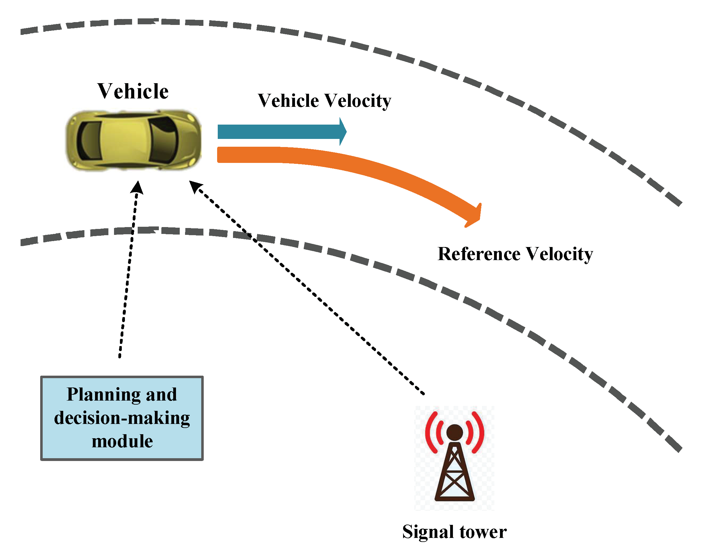
In recent decades, automated vehicles have developed rapidly, which are of great significance in improving driving comfort [1] and energy efficiency [2]. The automated driving system mainly includes positioning, perception, planning and decision-making, and control modules [3,4,5,6]. The planning and decision-making module decide the reference trajectory or reference velocity based on the information obtained by the sensing module and the state of the vehicle. The control module can track the reference trajectory or velocity by regulating the accelerator, brake, and steering wheel of vehicles.

Vehicle velocity tracking [7] is an important automated driving control, which can be considered as a simplified adaptive cruise control (ACC). Velocity tracking usually adopts the strategy of hierarchical control, where an upper decision-making layer calculates the reference velocity profile based on environment information. However, the sensor noise and the interaction of surrounding vehicles have great influence on decision-making. Therefore, a new distributed mean-field-type filter is proposed in [8] to handle noises, partial-observed and high-dimensional data, which improves the accuracy of vehicle tracking. Not only is a smoothing algorithm of the measured data proposed in [9] to reduce the impact of road surface and body vibration, but also an ACC system with traffic jam and active collision avoidance function is proposed. The lower control layer is responsible for designing controller based on vehicle dynamics. However, vehicle is a multiple-input multiple-output constrained dynamical system with strong coupling characteristics, that is, the longitudinal and lateral characteristics influence each other. Either lateral control [10,11] or longitudinal control [12,13] of vehicles ignores lateral and longitudinal dynamics coupling. Integrated longitudinal and lateral control is proposed in [14,15,16], which considers the coupling characteristics, but still designs longitudinal and lateral controllers separately. While vehicles are at a high speed, a large steering angle, and a small adhesion coefficient, vehicles with decoupling controllers will inevitably suffer from handling stability problems. Therefore, it is necessary to fully consider coupling characteristics, and to control the lateral and longitudinal motions simultaneously.

Compared with other controllers such as proportional integral [17] and linear quadratic regulator [18], model predictive control (MPC) [19,20,21] has been widely used in vehicle lateral and longitudinal coupling control since it can effectively deal with constraints. However, nonlinear model predictive control (NMPC) needs to solve nonconvex optimization problems at each time instant, which might lead to excessive computational burden.

In order to avoid to solve nonconvex optimization problems and reduce online computational burden of NMPC, linearization methods, such as local linearization [22], multi-model method [23], and feedback linearization [24], are commonly used. Local linearization is the most commonly used linearization method. However, the linear model based on Taylor expansion works only around its equilibrium point [25], and it is necessary to update the linear model and solve the Jacobian matrix at each time instant. The multi-model method builds several linear models which are suitable for different working areas, but it is hard to ensure stability due to (frequent) model switching [26]. Feedback linearization requires precise mathematical models [27].

Koopman operator theory [28] provides a new tool to perform linearization. Its basic idea is to lift a nonlinear system to an infinite-dimensional linear space, and obtain its global linear model accordingly without information loss. Compared with common linearization methods, Koopman operator has great advantages. The global linear model constructed by Koopman operator is valid for all working points, which is obviously different from local linearization and the multi-model method. That is, the continuous updating of linear model or model switching is avoided, and the computational burden is further reduced. In principle, Koopman operator is data-driven and can build a linear model based on system’s input and output data. Compared with feedback linearization, there is no need to establish an accurate mechanism model.

The infinite dimensional Koopman operator is difficult to implement, so dynamic mode decomposition (DMD), extended dynamic mode decomposition (EDMD), and deep neural network (DNN) are often used to approximate an infinite-dimensional Koopman operator in finite dimensions. DMD [29] and EDMD [30] approximate the action of the Koopman operator on a subspace of the observable space by sampling. DMD can only be applied to autonomous systems, and has been widely used in the analysis of complex flow phenomena due to its simple mathematical expression. Dynamic mode decomposition with control (DMDc) [31] can overcome this limitation. Theoretically, EDMD can better approximate Koopman eigenfunctions and Koopman operator. However, manual selection of lifting functions has great influence on approximation accuracy. DNN [32,33] avoids manual selection of lifting functions, and provides the possibility to achieve high approximation accuracy. DNN has the disadvantage of complex structure and time-consuming training, so DMDc and EDMD algorithms are widely used to approximate the Koopman operator in finite dimensions.

Koopman operator is widely used in analysis and control of nonlinear systems [34,35,36,37]. To apply Koopman operator to vehicle control, a global linear model is constructed directly based on the system’s data. Then, linear controllers based on the obtained global linear models are designed. For example, a “global” linear model of vehicle dynamics is obtained in [38] based on the EDMD algorithm. A linear MPC, named Koopman MPC, is proposed in [39] to accurately track the reference velocity. However, it fails while the yaw rate is changing. A three-state single-track model of vehicles with linear tires is considered in [40]. While the nonlinear characteristic of tires is obvious, i.e., in the scenario of a large steering angle or small road adhesion coefficient, good velocity tracking performance cannot be achieved by the proposed MPC scheme. A Koopman MPC is proposed in [41] for velocity tracking of vehicles, in which Koopman operators are represented by a deep neural network. The strategy has a large error in tracking the reference velocity, which might result in the deviation of the driving state of vehicles and the handling stability problems, in particular, when the curvature of the road is constantly changing.

In this paper, an automated driving model predictive control of vehicles is proposed, in which vehicle dynamics and nonlinearity of tires are approximated by an identified Koopman linear model. Furthermore, a linear MPC is designed to guarantee accurate and implementable velocity tracking. Note that, different from [42], tire nonlinearity is considered when establishing vehicle dynamics model, and the DMDc algorithm is compared with the EDMD algorithm in model accuracy and online computational burden.

The main contributions of this paper are as follows:

• Automated vehicle control is reduced to a reference velocity tracking problem, in which the reference signal is provided by the module of perception and planner. In order to reflect full operating conditions, nonlinear vehicle dynamics and nonlinear tires which represent the coupling characteristics of longitudinal and lateral dynamics are considered.
• Koopman operator theory is adopted to transform the nonlinear vehicle model and tire into a global linear model. Thus, the trade-off between prediction accuracy and online computational burden is achieved.

This paper is organized as follows: Vehicle dynamics is introduced in Section 2. MPC considering nonlinear vehicle dynamics and nonlinear tires is introduced in Section 3. Linear MPC based on the Koopman operator is discussed in Section 4. Section 5 presents simulation results. The paper is concluded in Section 6.

2. Problem Setup

Velocity tracking is an important part of classical cruise control. As shown in Figure 1, the goal of velocity tracking is to track the reference velocity profile accurately in real time by regulating the driving, braking, and steering of vehicles, when the reference vehicle velocity is determined by the planning and decision-making module. In this section, vehicle dynamics considering tire nonlinearity and the objective of velocity tracking control are introduced.

2.1. Vehicle Dynamics

The longitudinal, lateral, and yaw motion of vehicles are considered in this paper. Suppose that the vehicle is front-wheel steering and four-wheel driving, and vehicle dynamics considering the lateral and longitudinal coupling shown in Figure 2 is established.

According to Newton’s Second Law, the vehicle longitudinal, lateral and yaw dynamics can be expressed as:

$$\left\{\begin{array}{c}m{\dot{v}}_x-m{v}_y\omega =F_{lf}cos\delta -F_{sf}sin\delta +F_{lr}\hfill \\ m{\dot{v}}_y+m{v}_x\omega =F_{lf}sin\delta +F_{sf}cos\delta +F_{sr}\hfill \\ I_z\dot{\omega }=\left(F_{lf}sin\delta +F_{sf}cos\delta \right)l_f-F_{sr}{l}_r\hfill \end{array}\right.$$

(1)

where $v_x$, $v_y$, and $\omega$ are the longitudinal velocity, lateral velocity, and yaw rate of the vehicle, respectively, m is the mass of vehicles, $\delta$ is the front steering angle, $F_{lf}$ and $F_{lr}$ are the longitudinal forces of front and rear wheel, $F_{sf}$ and $F_{sr}$ are the lateral forces of front and rear wheel, $l_f$ and $l_r$ are distances of wheels from the center of gravity, and $I_z$ is the moment of inertia around yaw axis.

The dynamics of wheels is shown in Figure 3, which can be described accordingly by

$$\left\{\begin{array}{c}{\dot{\omega }}_f=\left(T_f-R_e{F}_{lf}\right)/J\hfill \\ {\dot{\omega }}_r=\left(T_r-R_e{F}_{lr}\right)/J\hfill \end{array}\right.$$

(2)

where ${\omega }_f$ and ${\omega }_r$ are angular velocity of front and rear tires, $R_e$ is the wheel rolling radius, J is the moment of inertia of wheel, and $T_f$ and $T_r$ are the total torque of front and rear wheel.

In this paper, the single track model of vehicle is adopted. The torque distribution mode is as follows: the front and rear axles are distributed equally in driving and braking condition. Define T as the total torque of the vehicle. Then, the torque $T_f$ and $T_r$ can be expressed as

$$T_f=T_r=T/2$$

(3)

A five-degree-of-freedom (5DOF) model of vehicles is obtained by combining (1)–(3)

$$\left\{\begin{array}{c}m{\dot{v}}_x-m{v}_y\omega =F_{xf}cos\delta -F_{yf}sin\delta +F_{xr}\hfill \\ m{\dot{v}}_y+m{v}_x\omega =F_{xf}sin\delta +F_{yf}cos\delta +F_{yr}\hfill \\ I_z\dot{\omega }=\left(F_{xf}sin\delta +F_{yf}cos\delta \right)l_f-F_{yr}{l}_r\hfill \\ {\dot{\omega }}_f=\left(T/2-R_e{F}_{xf}\right)/J\hfill \\ {\dot{\omega }}_r=\left(T/2-R_e{F}_{xr}\right)/J\hfill \end{array}\right.$$

(4)

Denote the state of the system as $x={\left[v_x,v_y,\omega ,{\omega }_f,{\omega }_r\right]}^T$, the control input as $u={\left[\delta ,T\right]}^T$, and the output as $y={\left[v_x,v_y,\omega \right]}^T$. Thus, the vehicle dynamics (4) can be rewritten as

$$\left\{\begin{array}{c}\dot{x}=f(x,u)\hfill \\ y=Cx\hfill \end{array}\right.$$

(5)

where $x\in {\mathbb{R}}^5$, $u\in {\mathbb{R}}^2$, $C=\left[I_{3\times 3},0_{3\times 2}\right]$, I is an identity matrix, and $f:{\mathbb{R}}^5\times {\mathbb{R}}^2\to {\mathbb{R}}^3$ represents the related nonlinear mapping. Furthermore, the discrete counterpart of vehicle dynamics (5) is

$$\left\{\begin{array}{c}x\left(k+1\right)=f^{\prime }\left(x\left(k\right),u\left(k\right)\right)\hfill \\ y\left(k\right)=Cx\left(k\right)\hfill \end{array}\right.$$

(6)

provided that the sampling time is $T_s$.

2.2. Nonlinear Tire Model

Tires are the key components of vehicles which carry all the loads and influence handling stability. Under different vertical forces $F_n$, the relationship between slip ratio and longitudinal force is shown in Figure 4, and the relationship between slip angle and lateral force is shown in Figure 5. It can be seen from Figure 5 that, when the slip angle is small, the slip angle and lateral force is in an approximate linear relationship; as the slip angle increases, lateral force is saturated. That is, the small-angle approximation method [43] is no longer applicable while vehicles are fast steering at a high speed.

In order to accurately reflect the nonlinear properties of tires, the longitudinal and lateral tire force is calculated by the following magic formula [44]:

$$\left\{\begin{array}{c}{F}_l=D_{l}sin\left(C_{l}arctan\left(B_l{\alpha }_{f/r}-E_l\left(B_l{\alpha }_{f/r}-arctan{B}_l{\alpha }_{f/r}\right)\right)\right)\\ F_s=D_{s}sin\left(C_{s}arctan\left(B_s{k}_{f/r}-E_s\left(B_s{k}_{f/r}-arctan{B}_s{k}_{f/r}\right)\right)\right)\end{array}\right.$$

(7)

where $B_l$, $C_l$, $D_l$, $E_l$ and $B_s$, $C_s$, $D_s$, $E_s$ are magic formula parameters of the longitudinal tire force $F_l$ and lateral tire force $F_s$, respectively, ${\alpha }_f$ and ${\alpha }_r$ are the front and rear tire slip angles, and $k_f$ and $k_r$ are the front and rear tire slip ratios. The tire slip angle and slip ratio can be calculated by

$$\left\{\begin{array}{c}{\alpha }_f=arctan\left(\frac{v_{fy}^w}{v_{fx}^w}\right)\hfill \\ {\alpha }_r=arctan\left(\frac{v_{ry}^w}{v_{rx}^w}\right)\hfill \end{array}\right.$$

(8)

$$\left\{\begin{array}{c}{k}_f=\frac{{\omega }_f{R}_e-v_{fx}^w}{\left|v_{fx}^w\right|}\hfill \\ k_r=\frac{{\omega }_r{R}_e-v_{rx}^w}{\left|v_{rx}^w\right|}\hfill \end{array}\right.$$

(9)

where $v_{fx}^w$, $v_{fy}^w$, $v_{rx}^w$, and $v_{ry}^w$ are the longitudinal and lateral velocity of the front and rear wheels under the tire coordinate system.

Wheel velocities $v_{fx}^w$, $v_{fy}^w$, $v_{rx}^w$ and $v_{ry}^w$ can be expressed as:

$$\left\{\begin{array}{c}{v}_{fy}^w=v_{fy}cos\delta -v_{fx}sin\delta \hfill \\ v_{fx}^w=v_{fy}sin\delta +v_{fx}cos\delta \hfill \\ v_{ry}^w=v_{ry}\hfill \\ v_{rx}^w=v_{rx}\hfill \end{array}\right.$$

(10)

where $v_{fx}$, $v_{fy}$, $v_{rx}$ and $v_{ry}$ are the longitudinal and lateral velocity of the front and rear wheels under the vehicle coordinate system, and

$$\left\{\begin{array}{c}{v}_{fx}=v_x\hfill \\ v_{fy}=v_y+l_f\omega \hfill \\ v_{rx}=v_x\hfill \\ v_{ry}=v_y-l_r\omega \hfill \end{array}\right.$$

(11)

where $l_f$ ($l_r$) is distance from the front (rear) axle to mass center of the vehicle.

2.3. Control Objective

The control objective of velocity tracking is to accurately track the reference velocity profile, that is, to ensure that vehicles drive at the reference velocity, i.e.,

$$\left\{\begin{array}{c}\underset{k\to \infty }{lim}∥v_x\left(k\right)-v_x^{ref}\left(k\right)∥=0\hfill \\ \underset{k\to \infty }{lim}∥v_y\left(k\right)-v_y^{ref}\left(k\right)∥=0\hfill \\ \underset{k\to \infty }{lim}∥\omega \left(k\right)-{\omega }^{ref}\left(k\right)∥=0\hfill \end{array}\right.$$

(12)

where $v_x^{ref}\left(k\right)$, $v_y^{ref}\left(k\right)$, and ${\omega }^{ref}\left(k\right)$ are the reference longitudinal velocity, lateral velocity, and yaw rate, respectively.

3. NMPC of Automated Vehicles

In this section, a nonlinear model predictive controller is proposed to solve the velocity tracking problem. Suppose that the reference velocity is $r\left(k\right)={\left[v_x^{ref}\left(k\right),v_y^{ref}\left(k\right),{\omega }^{ref}\left(k\right)\right]}^T$. In order to track the time-varying reference velocity signal, the following optimization problem will be solved at each time instant.

Problem 1.

$$\underset{U\left(k\right)}{minimize}J\left(x\left(k\right),r\left(k\right),U\left(k\right)\right)$$

(13)

s.t.

$$\begin{array}{c}{x}^p\left(k+i+1|k\right)=f^{\prime }\left(x^p\left(k+i|k\right),u\left(k+i|k\right)\right)\hfill \\ y^p\left(k+i|k\right)=C{x}^p\left(k+i|k\right)\hfill \\ x^p\left(k|k\right)=x\left(k\right)\hfill \\ x^p\left(k+i|k\right)\in \left[x_{min}^p,x_{max}^p\right]\hfill \\ u\left(k+i|k\right)\in \left[u_{min},u_{max}\right]\hfill \end{array}$$

(14)

where $x^p\left(k+i|k\right)$ and $y^p\left(k+i|k\right)$ are the predicted state and predicted output, N is the prediction horizon, $r\left(k\right)=\left[r\left(k|k\right),r\left(k+1|k\right),\dots ,r\left(k+N-1|k\right)\right]$ is the sequence of the reference signal, $U\left(k\right)=\left[u\left(k|k\right),u\left(k+1|k\right),\dots ,u\left(k+N-1|k\right)\right]$ is the sequence of the control input, $x_{min/max}^p$ and $u_{min/max}$ are constraints of the system state and control input.

In order to track the reference velocity profile while guaranteeing that the control action is as small as possible, both the tracking error of the prediction state to the reference signal and the control input are included in the cost function. That is, the cost function is chosen as:

$$J\left(x\left(k\right),r\left(k\right),U\left(k\right)\right)=\sum _{i=0}^{N-1}\left[{∥y^p\left(k+i|k\right)-r\left(k+i|k\right)∥}_Q^2+{∥u\left(k+i|k\right)∥}_R^2\right]$$

(15)

where Q and R are positive semi-definite weighting matrices.

Denote $U^{*}\left(k\right)=\left[u^{*}\left(k|k\right),u^{*}\left(k+1|k\right),\dots ,u^{*}\left(k+N-1|k\right)\right]$ and $J^{*}\left(x\left(k\right),r\left(k\right),U\left(k\right)\right)$ as the optimal control sequence and the related optimal cost function. The first element of $U^{*}\left(k\right)$, i.e., $u^{*}\left(k|k\right)$ will be applied to vehicles.

The optimal control input of NMPC summarized in Algorithm 1 will be obtained through the solution of Problem 1 at each time instant, in which the optimal cost function is achieved as well.Furthermore, the proposed NMPC scheme can attenuate model-plant mismatches and external disturbances since the optimization problem is solved in a receding horizon manner. However, as the involved optimization problem is nonlinear and nonconvex, the proposed NMPC might suffer problems of heavy computational burden and local minima, which will seriously deteriorate the obtained performance.

Algorithm 1 NMPC of automated vehicles

Input: The prediction horizon N, weighting matrices Q, R, and initial value of the state $x\left(k\right)$

Output: Optimal control input $u^{*}\left(k|k\right)$

1: for $k=0,1,\dots$ do

2:      Obtain the current state $x\left(k\right)$, and the reference signal $r\left(k\right)$

3:      Solve Problem 1 to obtain $U^{*}\left(k\right)$

4:      Apply $u^{*}\left(k|k\right)$ to the vehicle

5: end for

4. Koopman-Based MPC of Automated Vehicles

The vehicle dynamics emerges nonlinear and strong coupling characteristics. In this section, Koopman linear models are constructed based on DMDc and EDMD algorithms, respectively. The identified Koopman linear model is used to design a model predictive controller, where the involved optimization problem is a quadratic programming problem. Note that, in order to obtain the approximated linear model, vehicle dynamics (6) is treated as a “transparent box” here.

The core idea of the Koopman operator theory is to express the evolution of nonlinear dynamical systems through an infinite-dimensional linear operator [28]. Define $\kappa$ as the infinite-dimensional Koopman operator acting on the observation function $\phi$. Under the action of $\kappa$, the nonlinear evolution of vehicles can be transformed into a linear evolution:

$$\kappa \phi \left(x\left(k\right)\right)=\phi \left(x\left(k+1\right)\right)=\phi \left(f^{\prime }\left(x\left(k\right),u\left(k\right)\right)\right)$$

(16)

The infinite-dimensional Koopman operator $\kappa$ is difficult to realize in practice. When the Koopman operator is applied to a real controlled system, a finite-dimensional approximation of $\kappa$ is often carried out. In this paper, the DMDc algorithm and the EDMD algorithm, two common methods to approximate the Koopman operator in finite dimensions, are applied to construct the global linear model of vehicles.

4.1. DMDc-MPC

The traditional DMD algorithm is only suitable for describing autonomous systems. Instead, the DMDc algorithm [31] extends the traditional DMD algorithm to systems under control. Construction of a Koopman linear model and a linear MPC based on the DMDc algorithm will be introduced in this subsection.

Based on the DMDc algorithm, the vehicle dynamics (6) can be approximated by a discrete linear model:

$$\left\{\begin{array}{c}\widehat{x}\left(k+1\right)=A_{DMD}\widehat{x}\left(k\right)+B_{DMD}u\left(k\right)\hfill \\ {\widehat{y}}_{DMD}\left(k\right)=C_{DMD}\widehat{x}\left(k\right)\hfill \end{array}\right.$$

(17)

where $\widehat{x}\left(k\right)\in {\mathbb{R}}^5$ and ${\widehat{y}}_{DMD}\left(k\right)\in {\mathbb{R}}^3$ are the state and output of the constructed linear model, respectively, the matrix $C_{DMD}$ is set to $\left[I_{3\times 3},0_{3\times 2}\right]$, and the matrices $A_{DMD}\in {\mathbb{R}}^{5\times 5}$ and $B_{DMD}\in {\mathbb{R}}^{5\times 2}$ are the parametric matrices that need to be identified.

In order to identify $A_{DMD}$ and $B_{DMD}$, collect state and control input data of the vehicle dynamics (6), and construct the following data matrices:

$$\begin{array}{c}{X}_1=\left[x\left(1\right),\cdots ,x\left(k_{max}\right)\right]\hfill \\ X_2=\left[x\left(2\right),\cdots ,x\left(k_{max}+1\right)\right]\hfill \\ Y=\left[y\left(1\right),\cdots ,y\left(k_{max}\right)\right]\hfill \\ U=\left[u\left(1\right),\cdots ,u\left(k_{max}\right)\right]\hfill \end{array}$$

(18)

where $X_1\in {\mathbb{R}}^{5\times k_{max}}$, $X_2\in {\mathbb{R}}^{5\times k_{max}}$, $Y\in {\mathbb{R}}^{3\times k_{max}}$, $U\in {\mathbb{R}}^{2\times k_{max}}$, and $k_{max}$ is the number of snapshots.

According to the Koopman linear model (17), the constructed data matrices can be expressed as:

$$X_2=\left[\begin{array}{cc}{A}_{DMD}& B_{DMD}\end{array}\right]\left[\begin{array}{c}{X}_1\\ U\end{array}\right]:=G\mathsf{\Omega }$$

(19)

where $G=\left[\begin{array}{cc}{A}_{DMD}& B_{DMD}\end{array}\right]$ is a finite-dimensional approximate matrix of the Koopman operator, and $\mathsf{\Omega }={\left[\begin{array}{cc}{X}_1& U\end{array}\right]}^T$ is a reconstructed augmented data matrix.

Perform singular value decomposition (SVD) on matrix $\mathsf{\Omega }$. Denote the truncated rank of SVD as p. In this paper, set $p=5$. The matrix $\mathsf{\Omega }$ can be expressed as

$$\mathsf{\Omega }\approx \tilde{U}\tilde{\mathsf{\Sigma }}{\tilde{V}}^T$$

(20)

where $\tilde{U}\in {\mathbb{R}}^{(5+2)\times 5}$ is the unitary matrix, and $\tilde{\mathsf{\Sigma }}\in {\mathbb{R}}^{5\times 5}$ is a diagonal matrix.

To obtain the matrices $A_{DMD}$ and $B_{DMD}$ from the matrix G, decompose the matrix $\tilde{U}$ as:

$$\tilde{U}=\left[\begin{array}{c}{\tilde{U}}_1\\ {\tilde{U}}_2\end{array}\right]$$

(21)

where ${\tilde{U}}_1\in {\mathbb{R}}^{5\times 5}$ and ${\tilde{U}}_2\in {\mathbb{R}}^{2\times 5}$.

Thus, the matrices $A_{DMD}$ and $B_{DMD}$ in the Koopman linear model can be expressed as:

$$\begin{array}{c}{A}_{DMD}=X_2\tilde{V}{\tilde{\mathsf{\Sigma }}}^{-1}{\tilde{U}}_1^T\hfill \\ B_{DMD}=X_2\tilde{V}{\tilde{\mathsf{\Sigma }}}^{-1}{\tilde{U}}_2^T\hfill \end{array}$$

(22)

The finite-dimensional approximation of the Koopman operator using the DMDc algorithm is summarized in Algorithm 2.

Algorithm 2 Approximation of Koopman operator with DMDc algorithm

Require: Data of the state, output and control input of the vehicle dynamics $x\left(1\right),x\left(2\right),\cdots ,x\left(k_{max}+1\right)$, $y\left(1\right),y\left(2\right),\cdots ,y\left(k_{max}\right)$ and $u\left(1\right),\cdots ,u\left(k_{max}\right)$.

Ensure: The matrices $A_{DMD}$, $B_{DMD}$

1: Construct data matrices (18);

2: Construct $\mathsf{\Omega }={\left[X_1,U\right]}^T$ based on data matrices;

3: Perform singular value decomposition on the matrix $\mathsf{\Omega }$ by (20);

4: Decompose the matrix $\tilde{U}$ into ${\tilde{U}}_1$ and ${\tilde{U}}_2$ by (21), and calculate the matrices $A_{DMD}$, $B_{DMD}$ by (22).

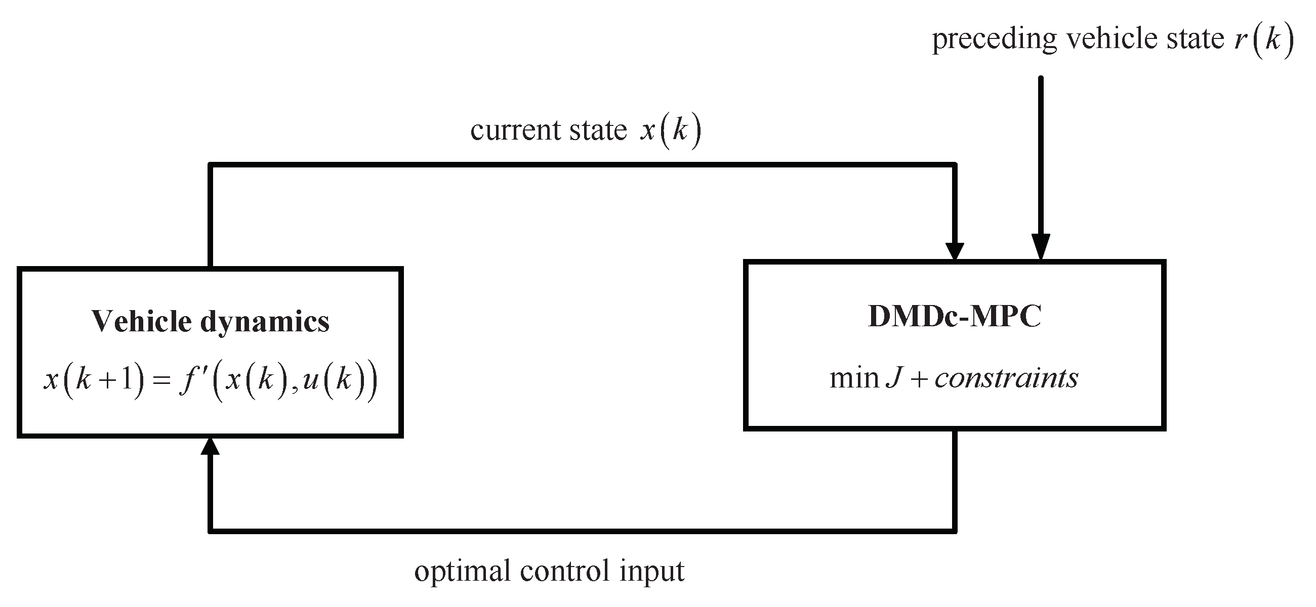
Based on the Koopman linear model (17), a linear model predictive controller, i.e., DMDc-MPC, is designed. The optimization problem of DMDc-MPC is as follows:

Problem 2.

$$\underset{U\left(k\right)}{minimize} J\left(\widehat{x}\left(k\right),r\left(k\right),U\left(k\right)\right)$$

(23)

s.t.

$$\begin{array}{c}\widehat{x}\left(k+i+1|k\right)=A_{DMD}\widehat{x}\left(k+i|k\right)+B_{DMD}u\left(k+i|k\right)\hfill \\ {\widehat{y}}_{DMD}\left(k+i|k\right)=C_{DMD}\widehat{x}\left(k+i|k\right)\hfill \\ \widehat{x}\left(k|k\right)=x\left(k\right)\hfill \\ \widehat{x}\left(k+i|k\right)\in \left[{\widehat{x}}_{min}^{DMD},{\widehat{x}}_{max}^{DMD}\right]\hfill \\ u\left(k+i|k\right)\in \left[u_{min}^{DMD},u_{max}^{DMD}\right]\hfill \end{array}$$

(24)

where $\widehat{x}\left(k+i|k\right)$ and ${\widehat{y}}_{DMD}\left(k+i|k\right)$ are the predicted state and predicted output based on the Koopman linear model (17), respectively, N is the prediction horizon, ${\widehat{x}}_{min/max}^{DMD}$, and $u_{min/max}^{DMD}$ are constraints of the system state and control input, and $U\left(k\right)$ is the sequence of the control input. The cost function can be expressed as:

$$J\left(\widehat{x}\left(k\right),r\left(k\right),U\left(k\right)\right)=\sum _{i=0}^{N-1}\left[{∥{\widehat{y}}_{DMD}\left(k+i|k\right)-r\left(k+i|k\right)∥}_{Q_{DMD}}^2+{∥u\left(k+i|k\right)∥}_{R_{DMD}}^2\right]$$

(25)

where $Q_{DMD}$ and $R_{DMD}$ are positive semi-definite weighting matrices.

The first element $u^{*}\left(k|k\right)$ of the optimal control sequence $U^{*}\left(k\right)$ will be applied to the vehicle to implement velocities’ tracking control.

The DMDc-MPC algorithm based on Koopman operator is summarized in Algorithm 3, and the related control diagram is shown in Figure 6.

Algorithm 3 DMDc-MPC based on Koopman operator

Input: The prediction horizon N, weighting matrices $Q_{DMD}$, $R_{DMD}$, parameter matrices $A_{DMD}$, $B_{DMD}$, $C_{DMD}$, and initial value of the system state $x\left(k\right)$

Output: optimal control input $u^{*}\left(k|k\right)$

1: for $k=0,1,\dots$ do

2:      Obtain the current state $x\left(k\right)$, and the reference signal $r\left(k\right)$

3:      Solve Problem 2, and obtain $U^{*}\left(k\right)$

4:      Apply $u^{*}\left(k|k\right)$ to the vehicle system

5: end for

4.2. EDMD-MPC

The EDMD algorithm [36] provides another idea for extending the traditional Koopman operator to the controlled system. The Koopman operator of the controlled system is defined as the Koopman operator of the autonomous system that evolves on a lifted state space.

Denote control to go as $\mathbf{u}\left(k\right):=u{\left(i\right)}_{i=k}^{\infty }$. Set the lifted state space as the combination of the current system state and control to go, i.e., $\chi \left(k\right)={\left[x\left(k\right),\mathbf{u}\left(k\right)\right]}^T$. The evolution of the lifted state $\chi \left(k\right)$ is

$$\chi \left(k+1\right)=F\left(\chi \left(k\right)\right)=\left[\begin{array}{c}{f}^{\prime }\left(x\left(k\right),u\left(k\right)\right)\\ S\mathbf{u}\left(k\right)\end{array}\right]$$

(26)

where $F\left(·\right)$ represents the nonlinear mapping from $\chi \left(k\right)$ to $\chi \left(k+1\right)$, and S is the left shift operator for updating the control sequence, i.e., $\mathbf{u}\left(k+1\right)=S\mathbf{u}\left(k\right)$.

Define ${\kappa }^{\prime }$ as the Koopman operator acting on the observation function ${\phi }^{\prime }\left(\chi \left(k\right)\right)$, i.e.,

$${\kappa }^{\prime }{\phi }^{\prime }\left(\chi \left(k\right)\right)={\phi }^{\prime }\left(F\left(\chi \left(k\right)\right)\right)$$

(27)

The approximation of the Koopman operator ${\kappa }^{\prime }$ of the vehicle dynamics (6) is obtained by solving the least squares optimization problem:

$$\underset{A_{EDMD},B_{EDMD}}{minimize}\sum _{k=1}^{k_{max}}{∥\psi \left(x\left(k+1\right)\right)-A_{EDMD}\psi \left(x\left(k\right)\right)-B_{EDMD}u\left(k\right)∥}_2^2$$

(28)

where $\psi \left(x\left(k\right)\right)={\left[{\psi }_1\left(x\left(k\right)\right),{\psi }_2\left(x\left(k\right)\right),\dots ,{\psi }_{N_{\psi }}\left(x\left(k\right)\right)\right]}^T$ is the vector of selected lifting functions, $A_{EDMD}\in {\mathbb{R}}^{N_{\psi }\times N_{\psi }}$ and $B_{EDMD}\in {\mathbb{R}}^{N_{\psi }\times 2}$ are the coefficient matrices to be calculated, and $N_{\psi }$ is the number of lifting functions with $N_{\psi }\gg 5$.

After solving the optimization problem (28), the discrete linear model of vehicles can be constructed as:

$$\left\{\begin{array}{c}z\left(k+1\right)=A_{EDMD}z\left(k\right)+B_{EDMD}u\left(k\right)\hfill \\ {\widehat{y}}_{EDMD}\left(k\right)=C_{EDMD}z\left(k\right)\hfill \end{array}\right.$$

(29)

where $z\left(k\right)\in {\mathbb{R}}^{N_{\psi }}$ and ${\widehat{y}}_{EDMD}\left(k\right)\in {\mathbb{R}}^3$ are the lifted state and output, respectively. The state $z\left(k\right)=\psi \left(x\left(k\right)\right):={\left[{\psi }_1\left(x\left(k\right)\right),{\psi }_2\left(x\left(k\right)\right),\dots ,{\psi }_{N_{\psi }}\left(x\left(k\right)\right)\right]}^T$. The matrix $C_{EDMD}\in {\mathbb{R}}^{3\times N_{\psi }}$ in (29) can be obtained by solving the following least squares optimization problem:

$$\underset{C_{EDMD}}{minimize}\sum _{k=1}^{k_{max}}{∥y\left(k\right)-C_{EDMD}\psi \left(x\left(k\right)\right)∥}_2^2$$

(30)

A finite-dimensional approximation of the Koopman operator using the EDMD algorithm is summarized in Algorithm 4.

Algorithm 4 Approximation of Koopman operator with the EDMD algorithm

Require: Data of state, output and control input of vehicle dynamics $x\left(1\right),x\left(2\right),\cdots ,x\left(k_{max}+1\right)$, $y\left(1\right),y\left(2\right),\cdots ,y\left(k_{max}\right)$ and $u\left(1\right),\cdots ,u\left(k_{max}\right)$, the selected lifting functions $\psi \left(x\right)={\left[{\psi }_1\left(x\right),\cdots ,{\psi }_{N_{\psi }}\left(x\right)\right]}^T$.

Ensure: The matrices $A_{EDMD}$, $B_{EDMD}$, $C_{EDMD}$

1: Construct the data matrices (18);

2: Lift the dimension of $X_1$ and $X_2$ with $\psi$ to obtain $X_{1,lift}$ and $X_{2,lift}$; $$\begin{array}{c}{X}_{1,lift}=\left[\psi \left(x\left(1\right)\right),\dots ,\psi \left(x\left(k_{max}\right)\right)\right]\hfill \\ X_{2,lift}=\left[\psi \left(x\left(2\right)\right),\dots ,\psi \left(x\left(k_{max}+1\right)\right)\right]\hfill \end{array}$$

3: Solve the optimization problem (28) and (30) to obtain $A_{EDMD}$, $B_{EDMD}$, $C_{EDMD}$.

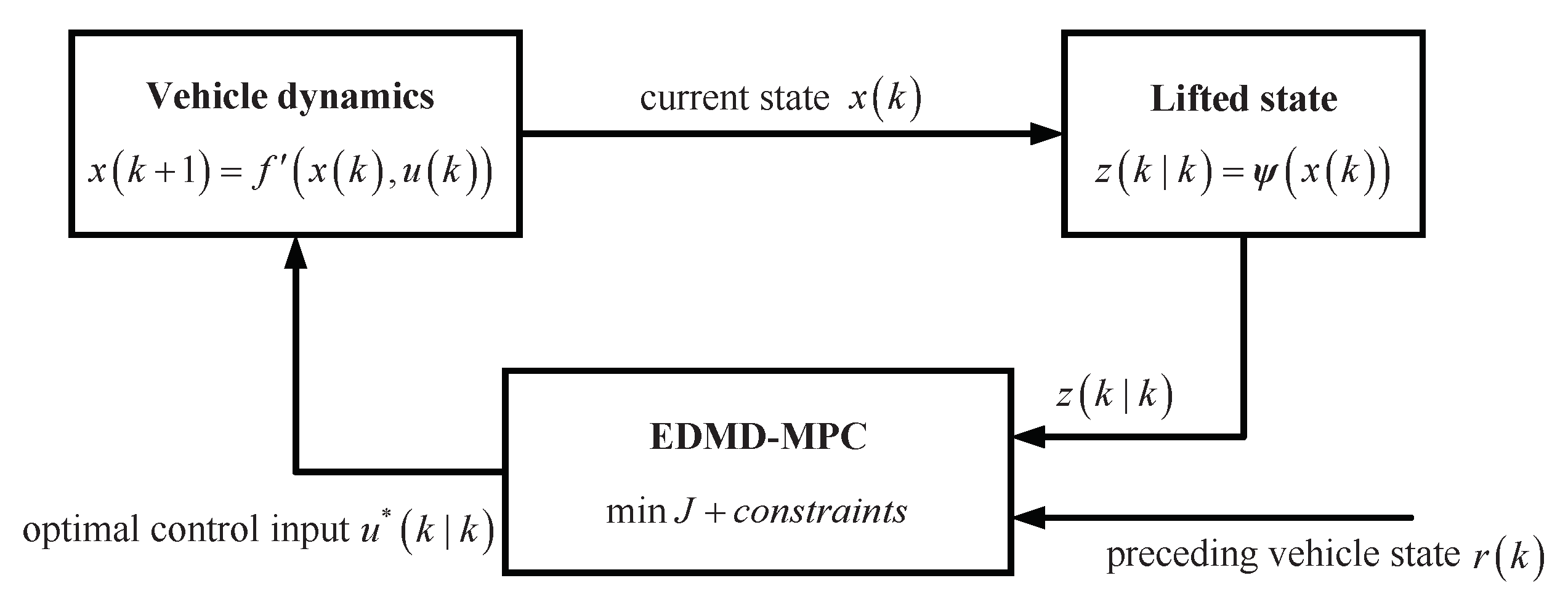
Based on the Koopman linear model (29), a linear model predictive controller, i.e., EDMD-MPC, is designed. The optimization problem of EDMD-MPC is as follows:

Problem 3.

$$\underset{U\left(k\right)}{minimize} J\left(z\left(k\right),r\left(k\right),U\left(k\right)\right)$$

(31)

s.t.

$$\begin{array}{c}z\left(k+i+1|k\right)=A_{EDMD}z\left(k+i|k\right)+B_{EDMD}u\left(k+i|k\right)\hfill \\ {\widehat{y}}_{EDMD}\left(k+i|k\right)=C_{EDMD}z\left(k+i|k\right)\hfill \\ z\left(k|k\right)=\psi \left(x\left(k\right)\right)\hfill \\ {\widehat{y}}_{EDMD}\left(k+i|k\right)\in \left[{\widehat{y}}_{min},{\widehat{y}}_{max}\right]\hfill \\ u\left(k+i|k\right)\in \left[u_{min}^{EDMD},u_{max}^{EDMD}\right]\hfill \end{array}$$

(32)

where $z\left(k+i|k\right)$ and ${\widehat{y}}_{EDMD}\left(k+i|k\right)={\left[{\widehat{v}}_x\left(k+i|k\right),{\widehat{v}}_y\left(k+i|k\right),\widehat{\omega }\left(k+i|k\right)\right]}^T$ are the predicted state and output based on the Koopman linear model (29), respectively, N is the prediction horizon, $U\left(k\right)$ is the sequence of the control input, ${\widehat{y}}_{min/max}$ and $u_{min/max}^{EDMD}$ are constraints, and the cost function can be expressed as:

$$J\left(z\left(k\right),r\left(k\right),U\left(k\right)\right)=\sum _{i=0}^{N-1}\left[{∥{\widehat{y}}_{EDMD}\left(k+i|k\right)-r\left(k+i|k\right)∥}_{Q_{EDMD}}^2+{∥u\left(k+i|k\right)∥}_{R_{EDMD}}^2\right]$$

(33)

where $Q_{EDMD}$ and $R_{EDMD}$ are positive semi-definite weighting matrices.

The EDMD-MPC algorithm based on Koopman operator is summarized in Algorithm 5, and the control diagram is shown in Figure 7.

Algorithm 5 EDMD-MPC based on Koopman operator

Input: The prediction horizon N, weight matrices $Q_{EDMD}$, $R_{EDMD}$, parameter matrices $A_{EDMD}$, $B_{EDMD}$, $C_{EDMD}$, and the initial value of the state $x\left(k\right)$

Output: optimal control input $u^{*}\left(k|k\right)$

1: for $k=0,1,\dots$ do

2:      Obtain the current state $x\left(k\right)$, and the reference signal $r\left(k\right)$

3:      Lift the dimension of the state $x\left(k\right)$ and obtain $z\left(k|k\right)$

4:      Solve Problem 3, and obtain $U^{*}\left(k\right)$

5:      Apply $u^{*}\left(k|k\right)$ to the vehicle system

6: end for

Remark 1.

Since it is difficult to directly collect data of vehicles to reflect the required dynamic characteristics due to safety consideration, the vehicle dynamics (6) is used as “data generator”. Thus, the proposed scheme is a hybrid mechanistic-data driven approach which can balance the computational burden of MPC and accuracy of prediction.

5. Simulation Results

In order to verify the effectiveness of the proposed scheme, simulation experiments are carried out in the Matlab R2016b environment. The Koopman linear model which can approximate vehicle dynamics is identified with the DMDc/EDMD algorithm, respectively. The effectiveness of the proposed model predictive controller with the approximated global linear model is verified under different driving scenarios.

The parameters of the vehicle model are shown in

Table 1. Vehicle parameters.

Parameter	Value	Unit
m	1820	kg
g	9.8	m/s2
$I_z$	4095	kg · m2
$l_f$	1.265	m
$l_r$	1.675	m
$R_e$	0.353	m
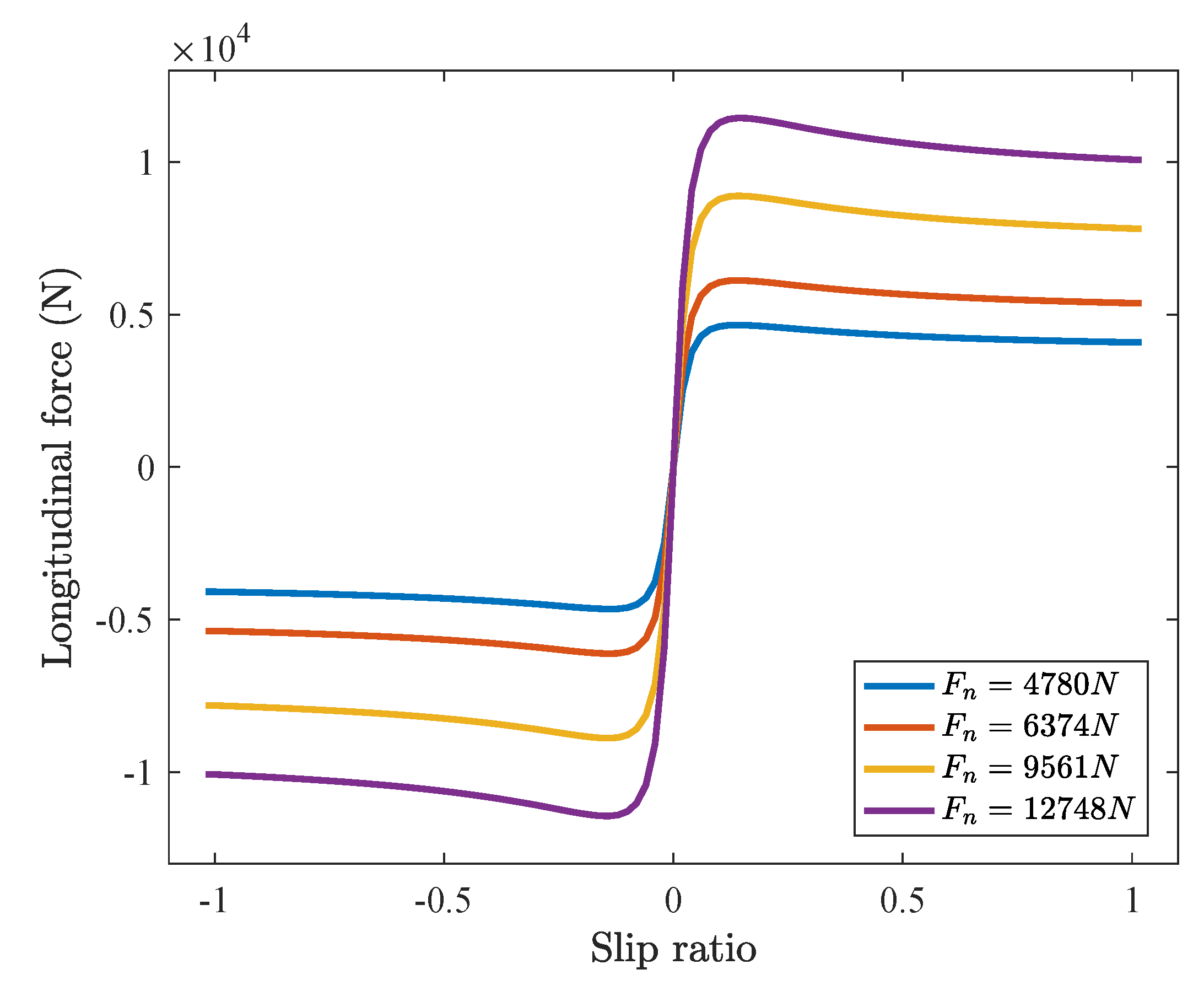
J	1	kg · m2

, and the parameters of the magic formula of tires are shown in

Table 2. Parameters of tire force.

Parameter	Front	Rear	Parameter	Front	Rear
$B_l$	14.27	14.33	$B_s$	7.937	8.036
$C_l$	1.921	1.923	$C_s$	2.205	2.205
$D_l$	4931	3762	$D_s$	4941	3769
$E_l$	0.9699	0.9702	$E_s$	1.004	1.004

.

5.1. Data Collection and Model Identification

In principle, Koopman operator theory is data-based, i.e., only input–output data are needed. However, vehicle dynamics (4) is used to ’produce’ data in this paper. That is, the proposed scheme is a kind of mixture of data-mechanism. In other words, measurement noise of sensors can be avoided indeed.

Set the sampling period $T_s$ to 10 ms, and discretize (5) using the Runge–Kutta method to obtain vehicle dynamics (6).

Select 1000 trajectories with the time duration of 2 s to form a dataset. In order to obtain data that can better reflect the dynamic characteristics of vehicles, 1000 trajectories in the dataset are divided equally to form a straight driving subdataset and a curve driving subdataset, respectively. The settings of the two subdatasets are as follows:

• Straight driving subdataset: The initial values of longitudinal velocity $v_x$, lateral velocity $v_y$, and yaw rate $\omega$ are randomly selected in $\left[1,30\right]$ m/s, $\left[-0.5,0.5\right]$ m/s, and $\left[-0.5,0.5\right]$ rad/s. The initial values of ${\omega }_f$ and ${\omega }_r$ are both randomly selected in $\left[1/R_e,30/R_e\right]$ rad/s. The torque T is randomly selected in $\left[-1000,1000\right]$ N, and the front steering angle $\delta$ is randomly selected in $\left[-0.001,0.001\right]$ rad.
• Curve driving subdataset: The initial values of longitudinal velocity $v_x$, lateral velocity $v_y$, and yaw rate $\omega$ are randomly selected in $\left[1,30\right]$ m/s, $\left[-0.5,0.5\right]$ m/s, and $\left[-0.5,0.5\right]$ rad/s. The initial values of ${\omega }_f$ and ${\omega }_r$ are both randomly selected in $\left[1/R_e,30/R_e\right]$ rad/s. The torque T is randomly selected in $\left[-600,600\right]$ N, and the front steering angle $\delta$ is randomly selected in $\left[-0.1,0.1\right]$ rad.

When using the EDMD algorithm to identify the Koopman linear model, a lifting function should be selected first. The lifting functions ${\psi }_i$ are chosen to be itself (i.e., ${\psi }_1=v_x$, ${\psi }_2=v_y$, ${\psi }_3=\omega$, ${\psi }_4={\omega }_f$, ${\psi }_5={\omega }_r$) and 100 Gaussian radial basis functions, so the dimension of the lifted state of the discrete linear model is 105. The expression of the Gaussian radial basis function is

$$m_y=exp\left(-\frac{{∥\theta -{\theta }_{center}∥}^2}{{\sigma }^2}\right)$$

(34)

where ${\theta }_{center}$ is the randomly selected center value, and $\sigma$ is the kernel width.

Remark 2.

While constructing the dataset, an approximate expression of the initial angular velocity of the front and rear tires is adopted, i.e., $v_x/R_e$. Thus, initial values of ${\omega }_f$ and ${\omega }_r$ are determined by the initial value of longitudinal velocity $v_x$ and tire radius $R_e$, that is, initial values of ${\omega }_f$ and ${\omega }_r$ are within $\left[1/R_e,30/R_e\right]rad/s$.

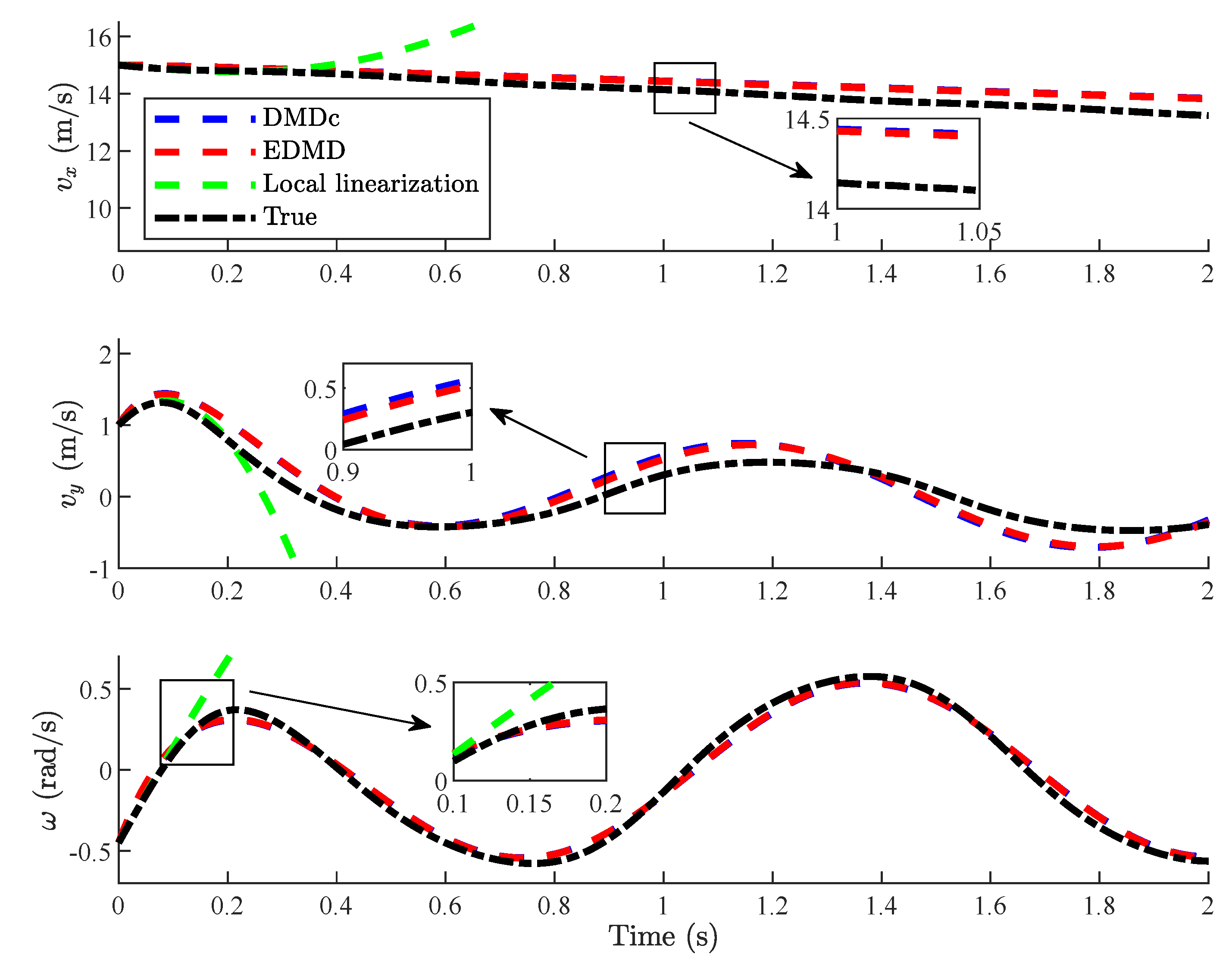
5.2. Model Validation

Here, simulation experiments are carried out to verify the effectiveness of the identified Koopman linear model through comparison of states of the actual vehicle system and the linear system approximated by the Koopman operator. Two scenarios are set as follows:

• Scenario 1 (longitudinal motion): The initial state of the vehicle system is set to ${\left[25,0,0,25/R_e,25/R_e\right]}^T$, the torque T is set to 600 Nm, and the front steering angle $\delta$ is set to 0.
• Scenario 2 (lateral and longitudinal coupling motion):The initial state of the vehicle system is set to ${\left[15,1,-0.45,15/R_e,15/R_e\right]}^T$, the torque T is set to $-400$ Nm, and the front steering angle is $\delta =0.15cos\left(5t\right)$.

Precision refers to how close the model’s predictions are to the observed values. The more precise the model, the closer the data point to the observed value. In order to test predicted precision, the Root Mean Square Error (RMSE ) is used as an objective evaluation index, i.e.,

$$RMSE=\frac{\sqrt{{\sum }_k{∥x_{pred}\left(k\right)-x_{true}\left(k\right)∥}_2^2}}{\sqrt{{\sum }_k{∥x_{true}\left(k\right)∥}_2^2}}\times 100\%$$

(35)

where $x_{true}\left(k\right)$ and $x_{pred}\left(k\right)$ are the actual state of vehicle system and the state of the identified Koopman linear model at time instant k, respectively.

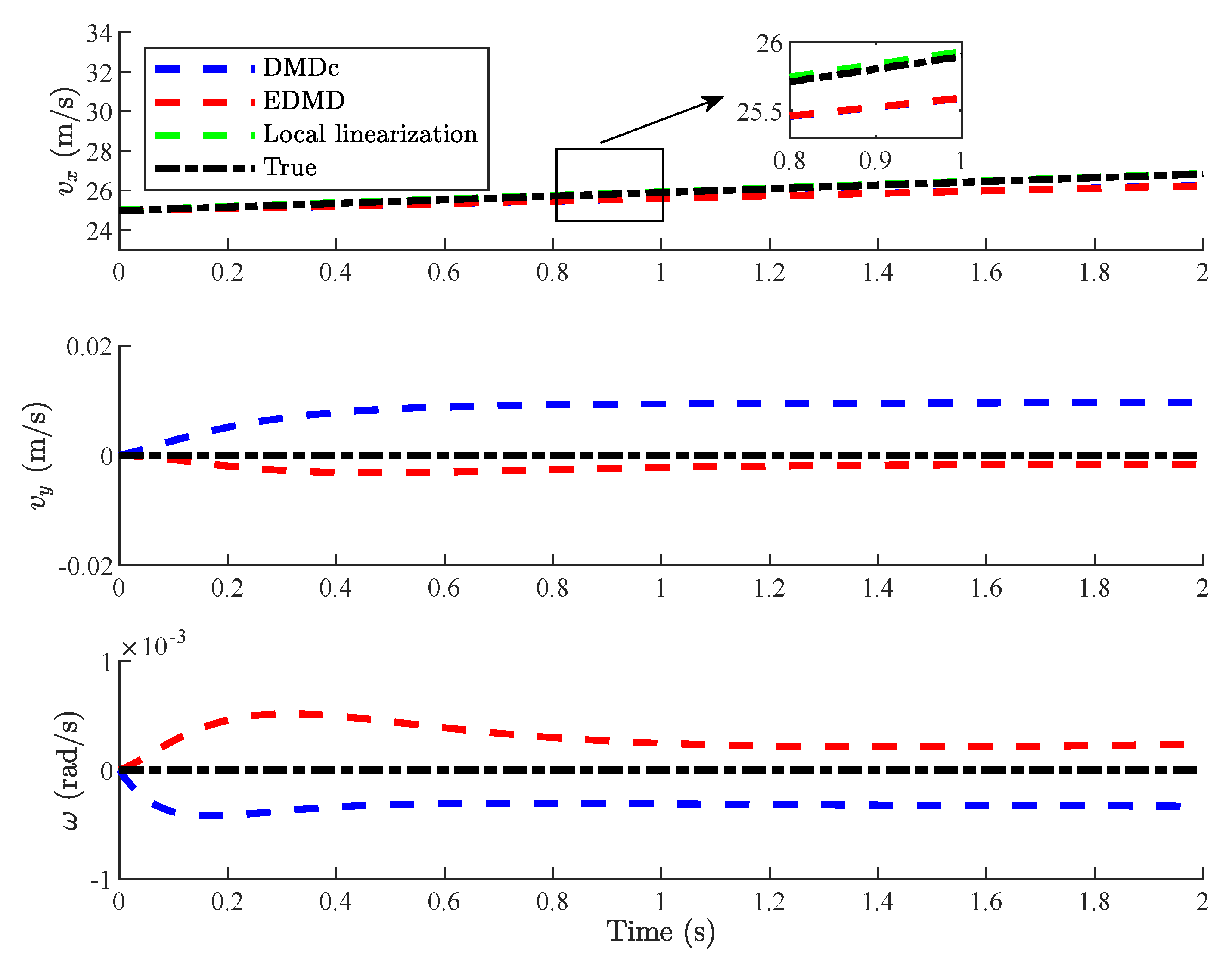
Under the two scenarios, the evolutions of local linearization and the identified Koopman linear models constructed by DMDc and EDMD algorithms are shown in Figure 8 and Figure 9. Accordingly, the values of RMSE of deviations between the real states and the predicted states with different methods are shown in

Table 3. RMSEs of deviations between the real states and the predicted states with different methods (Scenario 1).

Step N	10	30	50	100	200
DMDc	$0.09\%$	$0.28\%$	$0.43\%$	$0.74\%$	$1.32\%$
EDMD	$0.08\%$	$0.26\%$	$0.41\%$	$0.73\%$	$1.34\%$
Local linearization	$0.13\%$	$0.14\%$	$0.14\%$	$0.14\%$	$0.14\%$

and

Table 4. RMSEs of deviations between the real states and the predicted states with different methods (Scenario 2).

Step N	10	30	50	100	200
DMDc	$0.91\%$	$1.56\%$	$1.50\%$	$1.83\%$	$2.85\%$
EDMD	$0.88\%$	$1.54\%$	$1.49\%$	$1.73\%$	$2.73\%$
Local linearization	$0.15\%$	$2.98\%$	$13.97\%$	$71.48\%$	$238.20\%$

, respectively.

In Scenario 1, the front steering angle is set to 0, i.e., the coupling characteristics are weak. In this scenario, local linearization can achieve higher approximated accuracy than the Koopman linear model constructed by DMDc and EDMD algorithms.

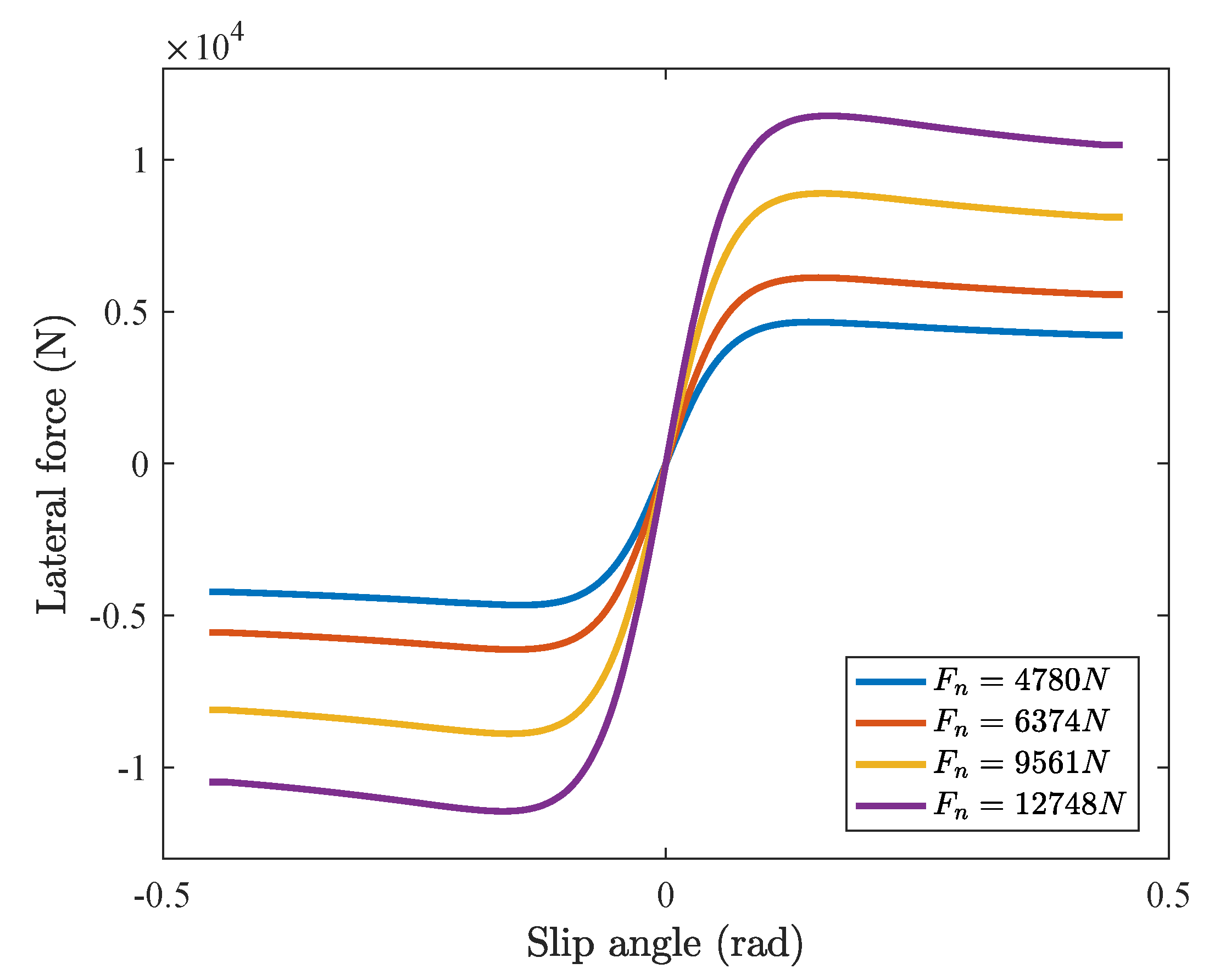
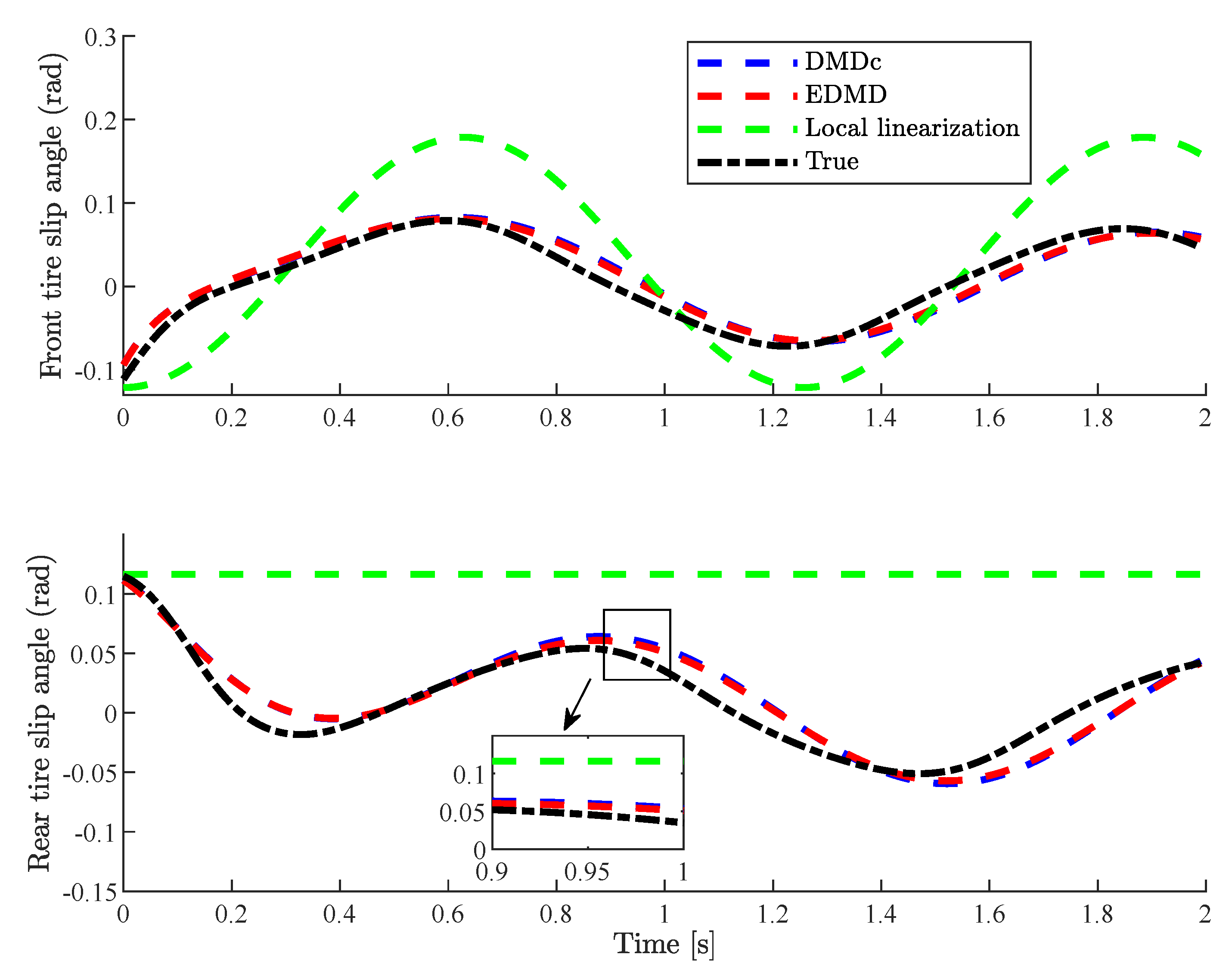
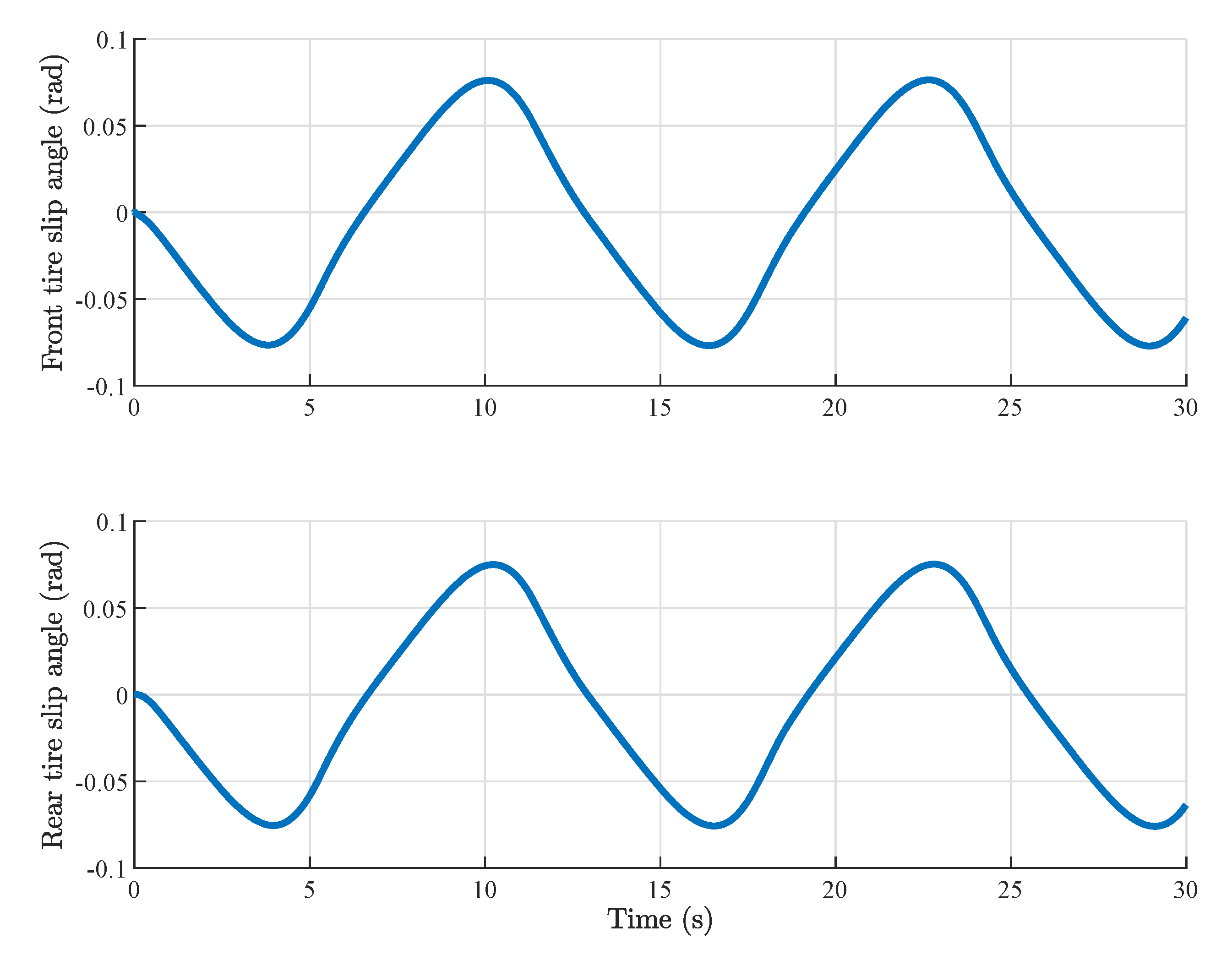
In Scenario 2, the front steering angle is time-varying, i.e., coupling characteristics are strong. As shown in Figure 10, in Scenario 2, the slip angle of the front and rear tires of the vehicle works in its nonlinear region. When coupling characteristics and tire nonlinearity are significant, the obtained Koopman linear model can approximate the system dynamics accurately. However, local linearization is failed.

Compared with local linearization, the data-driven Koopman linear model can predict the system dynamics accurately in various scenarios, especially in scenarios of strong tire nonlinearity. Compared with the DMDc algorithm, the Koopman linear model constructed by the EDMD algorithm has higher accuracy. However, the modeling process of EDMD algorithm is more complex, and the dimension of obtained Koopman linear model is much higher.

Note that, compared with [41], both nonlinear dynamics of vehicles and nonlinear characteristics of tires are considered in this paper.

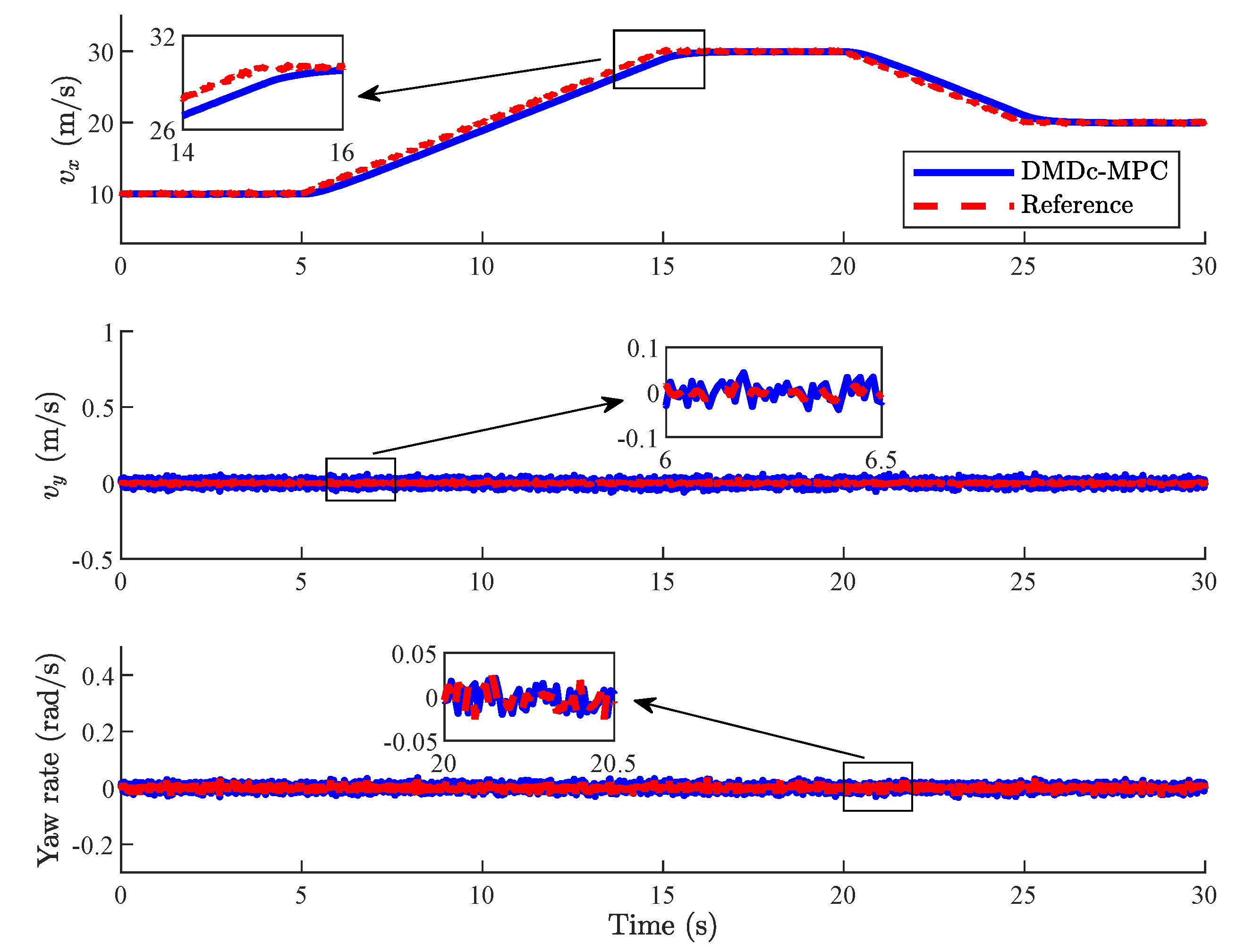
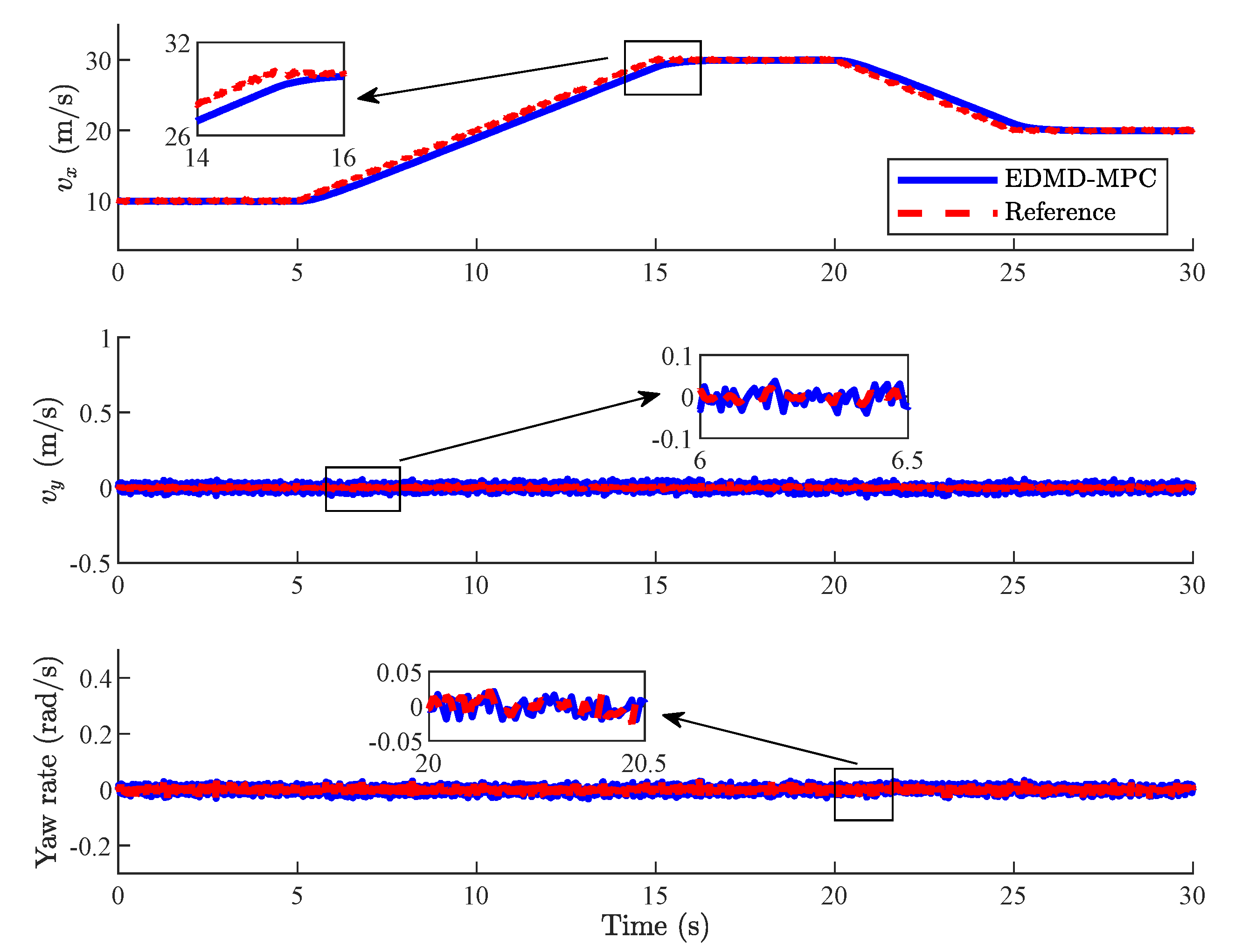
5.3. Velocity Tracking

In order to verify the effectiveness of both DMDc-MPC and EDMD-MPC, simulation experiments are carried out under three different cases:

• Case 1: The reference of the lateral velocity and yaw rate are set to 0, and the longitudinal velocity is time-varying. Note that the Gaussian distributed random signal is injected into the reference signal in this case.
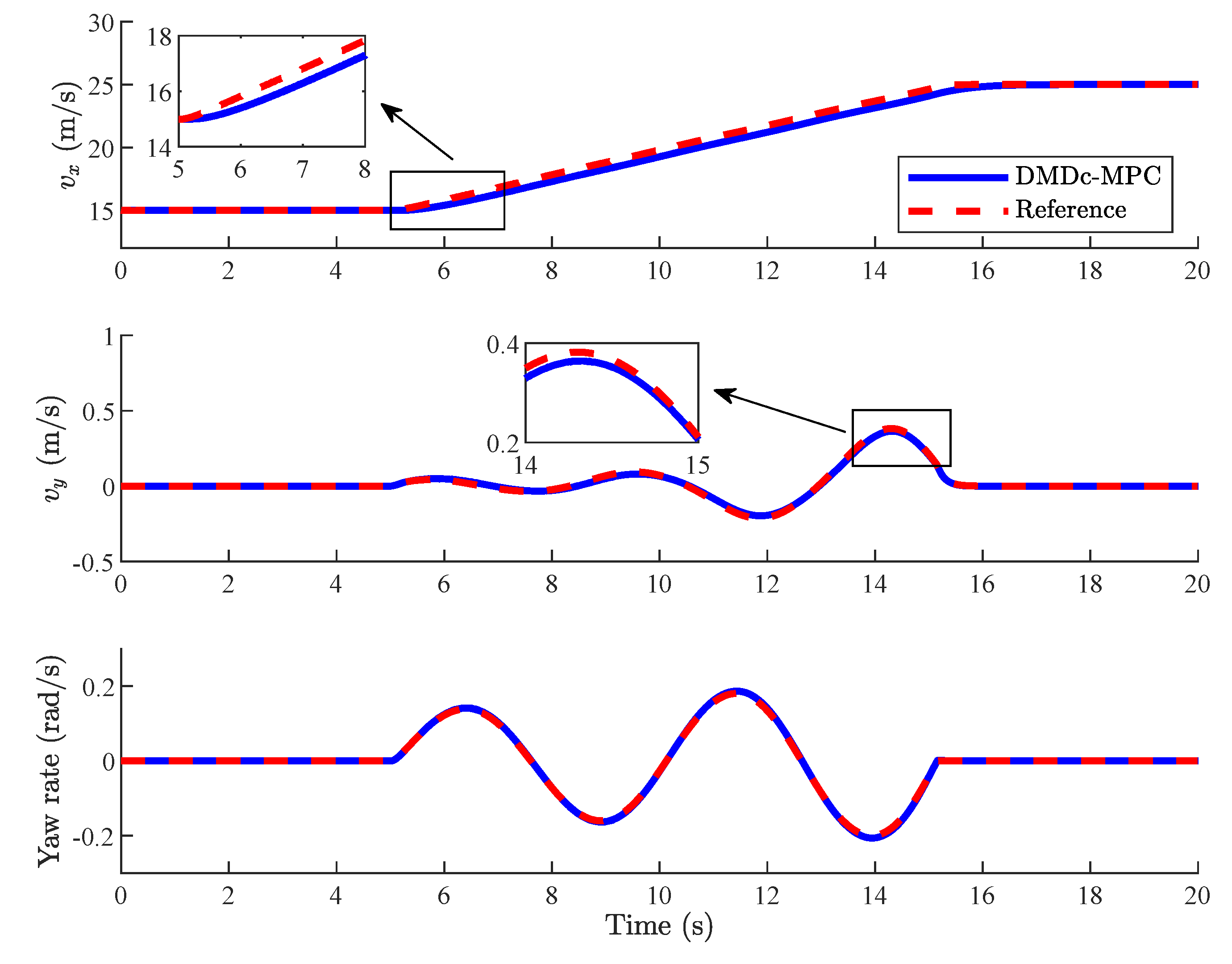
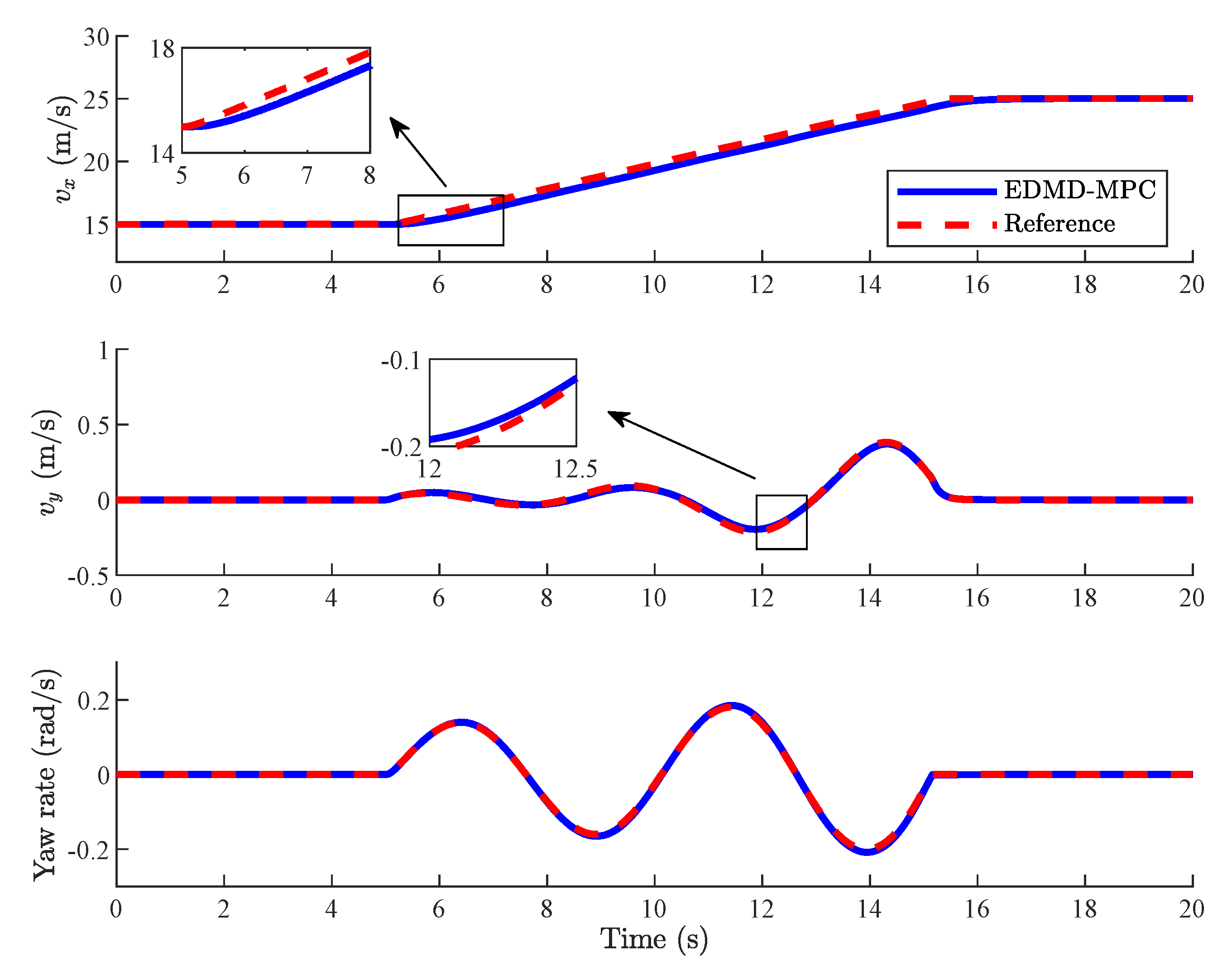
• Case 2: The reference of the lateral velocity and yaw rate are time-varying, and the longitudinal velocity persistently increases.
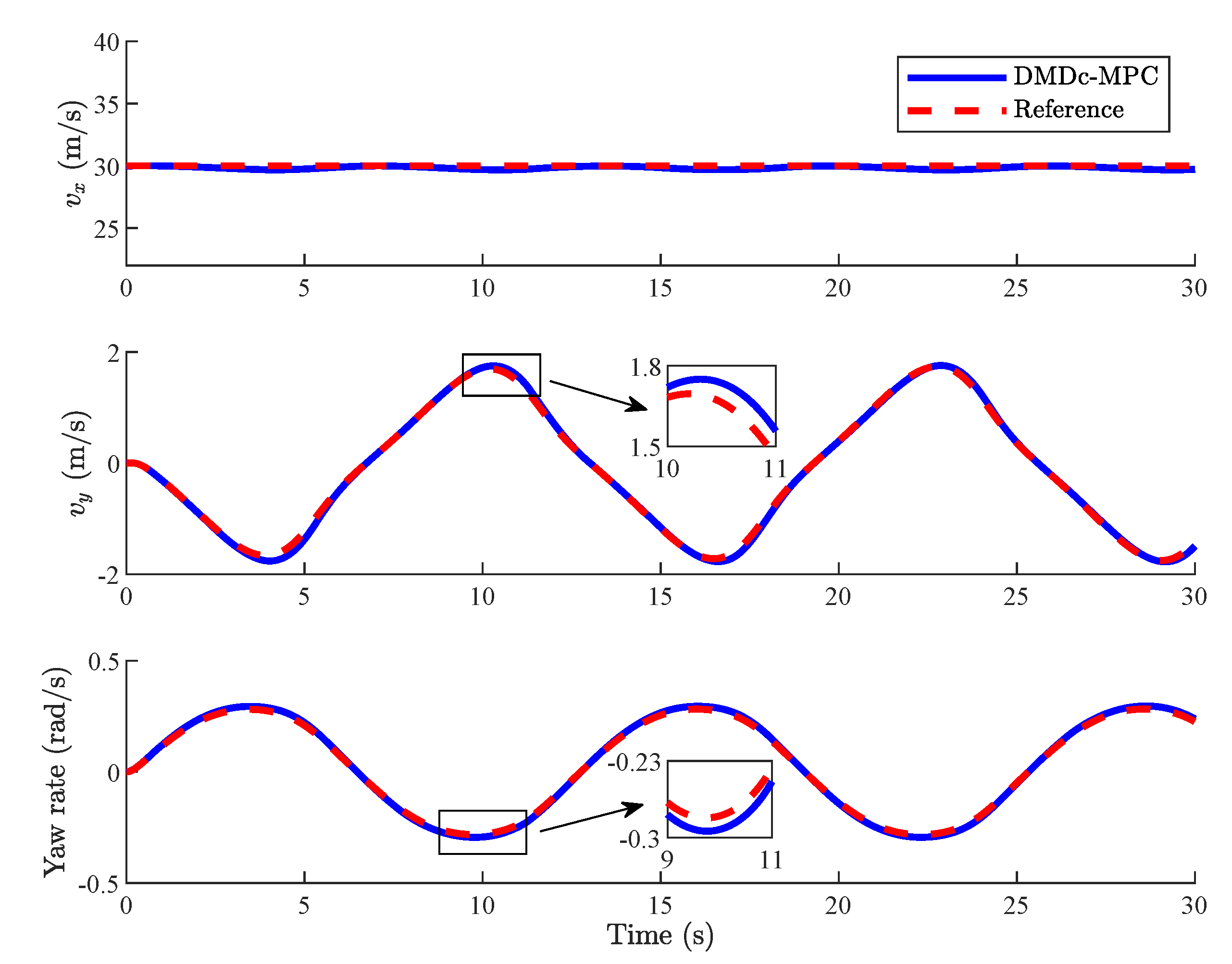
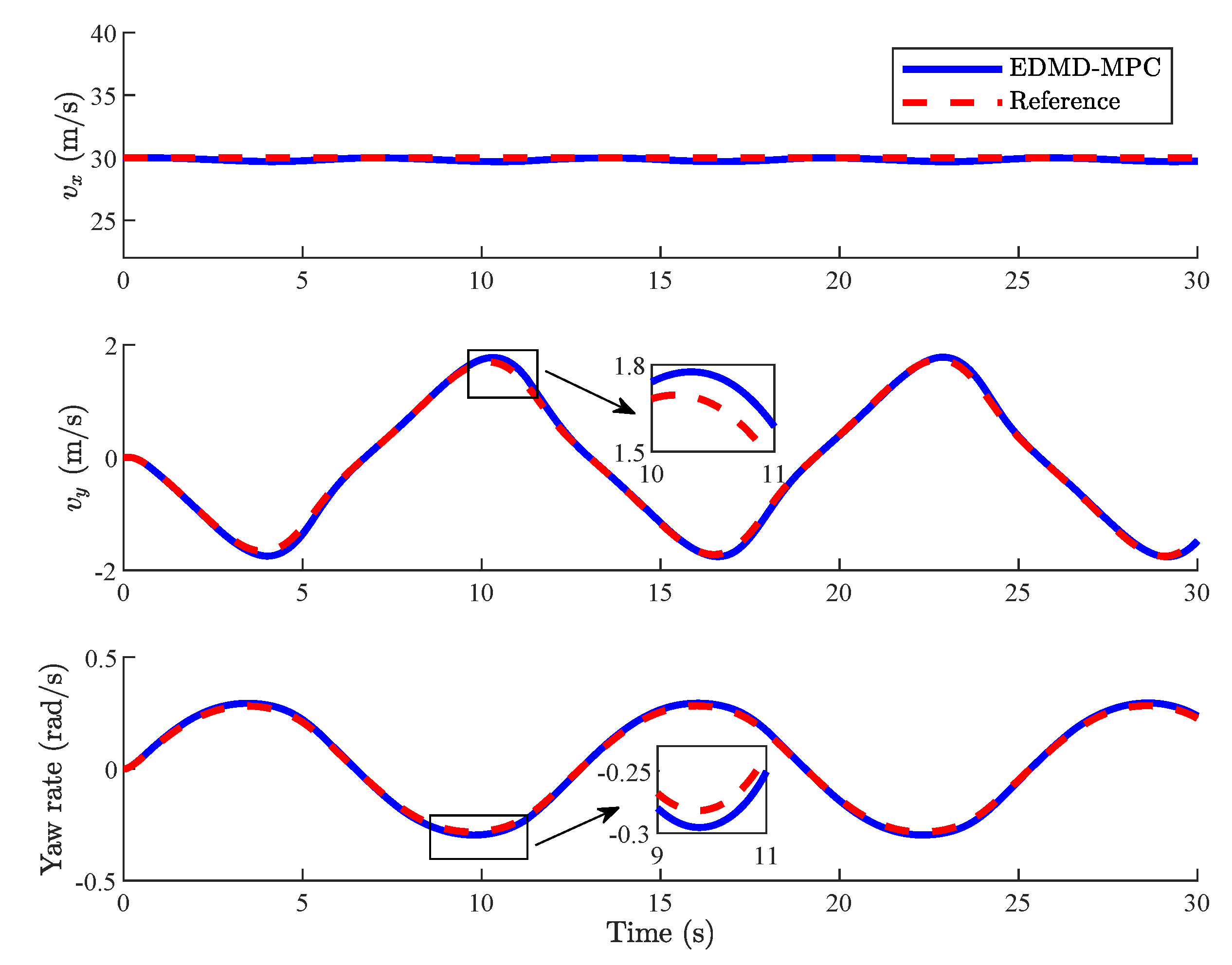
• Case 3: The reference of the lateral velocity and yaw rate are time-varying, and the longitudinal velocity is kept at 30 m/s.

Note that the reference velocities and the initial sate of vehicles are consistent in Case 1, 2, and 3.

Remark 3.

In this paper, only velocity tracking of reference is considered. Multi-sensor fusion, driver’s behavior, and the interaction of other vehicles in the traffic will be considered in future research.

Set the prediction horizon N to 10, and set the constraints of the longitudinal and lateral velocities and the yaw rate to $\left[-35,35\right]$ m/s, $\left[-2,2\right]$ m/s, and $\left[-1,1\right]$ rad/s. The constraints of the torque and the front steering angle are $\left[-1500,1500\right]$ Nm and $\left[-0.2,0.2\right]$ rad. The weight matrices are set as follows:

$$\begin{array}{c}{Q}_{DMD}=Q_{EDMD}=\left[\begin{array}{ccc}\mathrm{50,000}& 0& 0\\ 0& 500& 0\\ 0& 0& \mathrm{50,000}\end{array}\right]\hfill \\ R_{DMD}=R_{EDMD}=\left[\begin{array}{cc}0.1& 0\\ 0& 0.01\end{array}\right]\hfill \end{array}$$

(36)

Acceleration and deceleration in the longitudinal direction are considered in Case 1. Furthermore, measurement noise, i.e., Gaussian distribution with mean 0 and variance ${[{10}^{-2},{10}^{-4},{10}^{-4}]}^T$, is incorporated into the reference signals. Figure 11 and Figure 12 show that vehicles with both DMDc-MPC and EDMD-MPC can accurately track the reference velocity, and keep the lateral velocity and yaw rate close to zero.

Vehicles are accelerating at the longitudinal direction and changing lanes in Case 2, where the lateral and longitudinal motions are coupled. Since the lateral velocity is low, tire does not enter its nonlinear region, and the vehicle nonlinearity is mainly reflected in the lateral and longitudinal coupling characteristics. As shown in Figure 13 and Figure 14, vehicles with both DMDc-MPC and EDMD-MPC can effectively track the reference velocity signal with small deviation while the reference lateral velocity and yaw rate are changing. Compared with [40,41], the controller proposed in this paper makes the deviation between vehicle state and the reference velocity smaller, and the RMSE of deviations is about $10\%$ of [41].

Remark 4.

In cases of obvious lateral and longitudinal coupling characteristics, local linearization modeling fails to track the reference velocity signal. Furthermore, due to the complex structure of vehicle dynamics (6), updating the Jacobian matrix at each time instant will generate tremendous computational burden.

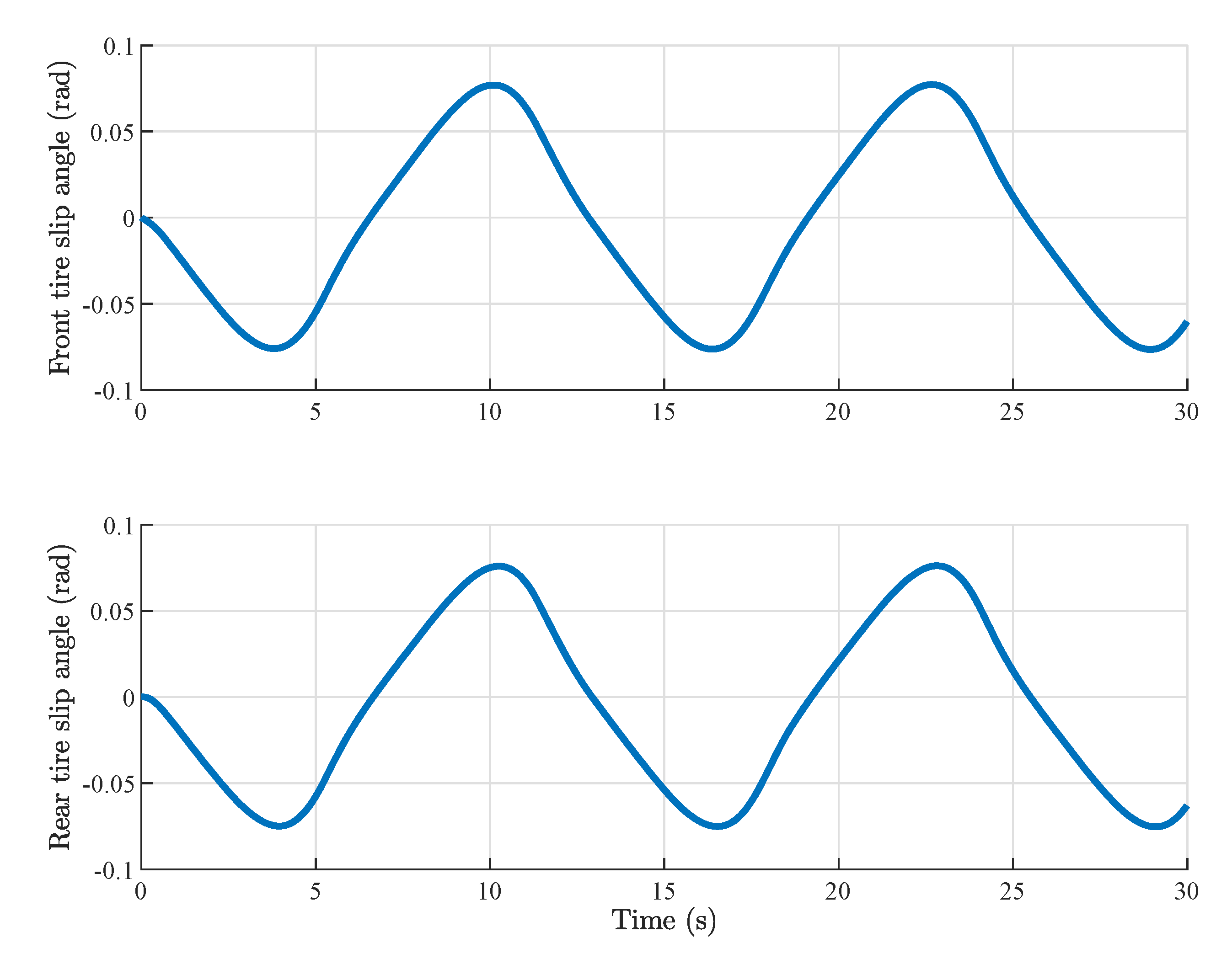
In order to verify the effectiveness of the proposed controller in scenario where the vehicle lateral and longitudinal coupling nonlinearity and tire nonlinearity are significant, the experiment in Case 3 is carried out. The designed controllers can effectively track the reference velocity signal, which is shown in Figure 15 and Figure 16. Furthermore, the slip angles of the front and rear tires of vehicles are shown in Figure 17 and Figure 18. When the slip angle of front and rear tires gradually reaches its peak, the nonlinear characteristic of tires emerges. The experimental results show that the proposed controller can still ensure tracking accuracy when the nonlinearity of the tire is significant.

RMSM of the proposed DMDc-MPC and EDMD-MPC in different cases is shown in

Table 5. RMSEs of tracking errors in different cases.

RMSE	DMDc-MPC	EDMD-MPC
Case 1	$3.44\%$	$3.29\%$
Case 2	$1.84\%$	$1.76\%$
Case 3	$0.68\%$	$0.65\%$

. The accuracy of the Koopman linear model based on the EDMD algorithm is higher, so the tracking accuracy of EDMD-MPC is slightly higher than that of DMDc-MPC.

The simulations are carried out with Processor Intel^® Core^TM i7-10700CPU @2.90 GHz produced by Intel^® Corporation, Santa Clara, CA, USA, and 16 GB RAM produced by Ramaxel Technology, Shenzhen, China. The optimization problem is solved by qpOASES [45]. The average computation time of the involved optimization problem is shown in

Table 6. Average computation time of DMDc-MPC and EDMD-MPC.

Computation Time (ms)	DMDc-MPC	EDMD-MPC
Case 1	$0.157$	$0.481$
Case 2	$0.162$	$0.463$
Case 3	$0.149$	$0.460$

, which is much smaller than the sampling time 10 ms. Compared with EDMD-MPC, DMDc-MPC can achieve similar performance with smaller computation time.

6. Conclusions and Future Research

In this paper, an efficient model predictive control for velocity tracking of automated vehicles was proposed, provided that a reference signal was given a priori. A 5-DOF nonlinear model of vehicles combined with nonlinear tires is introduced to cover full operation conditions. An approximated global linear model is obtained based on Koopman operator theory in order to reduce the online computational burden of MPC and avoid solving nonconvex/nonlinear optimization problems. The DMDc algorithm, EDMD algorithm, and the local linearization method are compared in different driving scenarios. Local linearization is only suitable for scenarios with weak coupling characteristics such as longitudinal driving scenarios. The Koopman linear model obtained by the DMDc algorithm and EDMD algorithm can guarantee the accurate prediction of system dynamics in various complex driving scenarios. The control strategy adopted in this paper can ensure the control accuracy and acceptable computational burden in complex scenarios with obvious coupling characteristics and tire nonlinearity, which is helpful to improve driving safety.

Future research will focus on adaptive cruise control and platooning of vehicles with a performance guarantee using efficient nonlinear model predictive control.