
Enhanced Marine Predators Algorithm for Solving Global Optimization and Feature Selection Problems
Abstract
:1. Introduction
- Improve the exploration phase of the MPA algorithm.
- Apply the “narrowed exploration” strategy of the AO in the MPA algorithm.
- Evaluate the proposed method using different optimization problems.
2. Related Work
3. Material and Methods
3.1. Marine Predators Algorithm (MPA)
- MPA initialization: As with all population-based algorithms, MPA has an initialization step where all populations are distributed uniformly in the search space as shown in Equation (1).where u and l are the lower and upper bounds, respectively. is a random vector in [0, 1]. The fittest solution is selected to form a matrix called Elite shown in Equation (2). Elite matrix has a dimension , where n is the search agents and n is the number of the problem dimension.Another matrix called Prey is constructed with the exact dimensions of Elite shown in Equation (3).The process of MPA is split into three levels based on the difference in velocity ratio between a predator and prey.
- Predator moving faster than prey (exploration phase): When the prey is faster than the predator, the predator’s best strategy is to remain stationary. Exploration is more important in the first third of iterations. The prey position is updated by a calculated as shown in Equation (4).where is a random numbers vector. The new prey position is updated as shown in Equation (5).where is a random vector in [0, 1].
- Predator and prey are moving at the same rate (exploitation vs. exploration):When the predator and the prey move at the same speed, they are both on the prowl for prey. This section occurs during the intermediate stage of the optimization process when exploration attempts to be transiently converted to exploitation. It is critical for both exploration and exploitation. As a result, half of the population is used for exploration and the other half is used for exploitation. During this phase, the predator is in charge of exploration, while the prey is in charge of exploitation. The new positions for the first half of the populations (supporting exploitation) are updated as shown in Equation (6).where is a vector of random numbers based on Levy distribution. The new positions for the second half of the populations (supporting exploration) are updated as shown in Equation (7)where A is a control parameter calculated as shown in Equation (8).
- Prey moving faster than predator (exploitation):This scenario occurs during the final stage of the optimization process and is typically associated with a high capacity for exploitation. The prey positions are updated as shown in Equation (9).To maintain the search, the Fish Aggregating Devices (FADs) is proposed. The mathematical model of FADs is defined in Equation (10). Algorithm 1 shows the pseudo code of the MPA.
| Algorithm 1 MPA pseudo code |
|
3.2. Aquila Optimizer (AO)
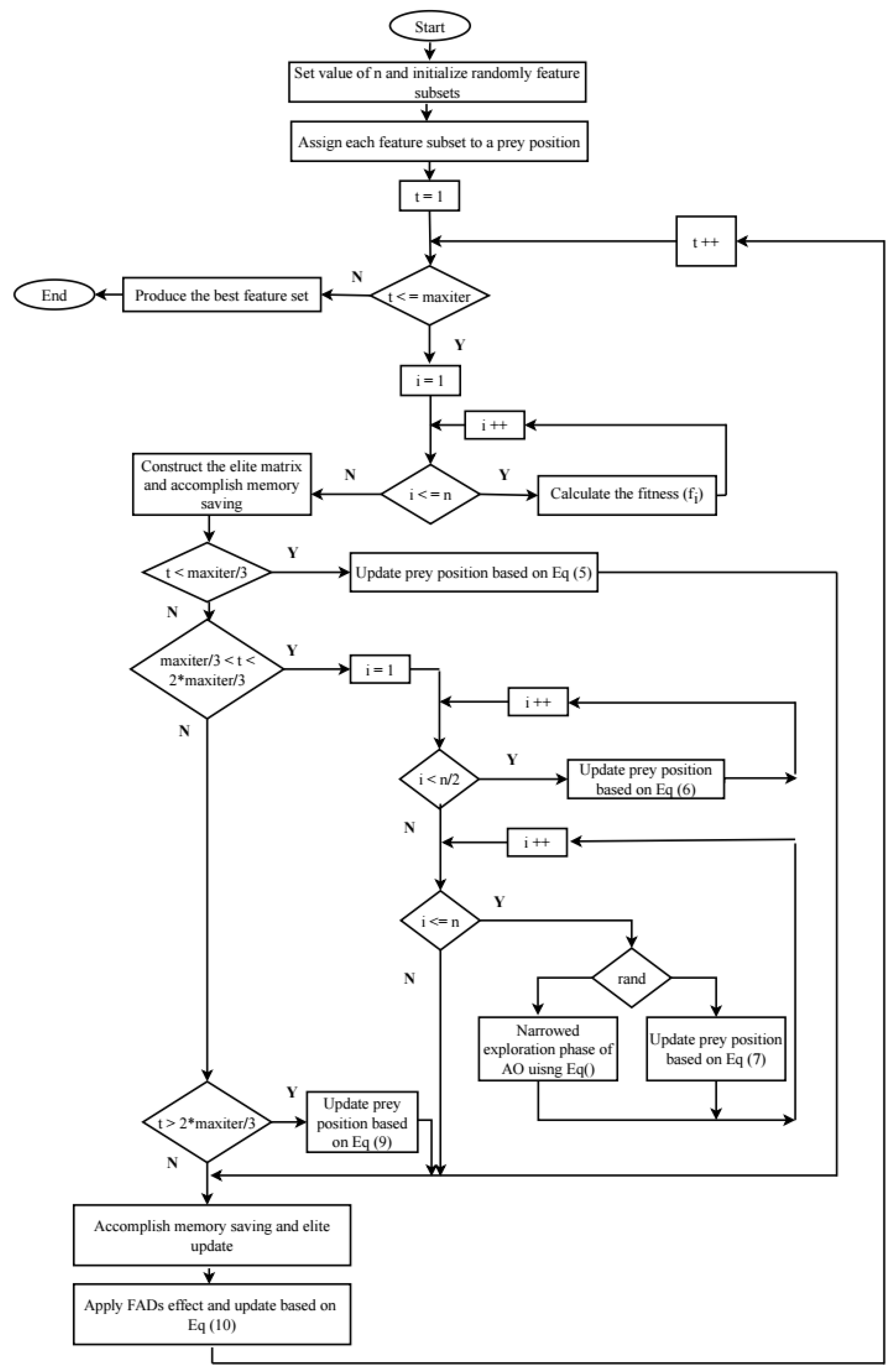
4. Proposed Method
- Declare the experiment variables and their values.
- Generate the X population randomly with a specific size and dimension.
- Start the main loop of the MPAO.
- Apply the fitness function for all solutions.
- Return the best value.
5. Experiments and Discussion
5.1. Experiment 1: Global Optimization
5.2. Experiment 2: Feature Selection
5.3. Experiment 3: Solving Different Real Engineering Problems
5.3.1. Tension/Compression Spring Problem
5.3.2. Rolling Element Bearing Problem
5.3.3. Speed Reducer Problem
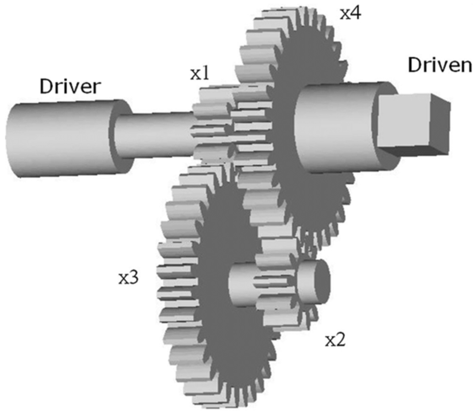
5.3.4. Gear Train Design Problem
6. Conclusions
Author Contributions
Funding
Data Availability Statement
Conflicts of Interest
References
- Kohavi, R.; John, G.H. Wrappers for feature subset selection. Artif. Intell. 1997, 97, 273–324. [Google Scholar] [CrossRef] [Green Version]
- Liu, H.; Motoda, H. Feature Extraction, Construction and Selection: A Data Mining Perspective; Springer Science & Business Media: Berlin/Heidelberg, Germany, 1998; Volume 453. [Google Scholar]
- Luukka, P. Feature selection using fuzzy entropy measures with similarity classifier. Expert Syst. Appl. 2011, 38, 4600–4607. [Google Scholar] [CrossRef]
- Talbi, E.G. Metaheuristics: From Design to Implementation; John Wiley & Sons: Hoboken, NJ, USA, 2009. [Google Scholar]
- Saremi, S.; Mirjalili, S.; Lewis, A. Grasshopper optimisation algorithm: Theory and application. Adv. Eng. Softw. 2017, 105, 30–47. [Google Scholar] [CrossRef] [Green Version]
- Hussien, A.G.; Amin, M. A self-adaptive Harris Hawks optimization algorithm with opposition-based learning and chaotic local search strategy for global optimization and feature selection. Int. J. Mach. Learn. Cybern. 2022, 13, 309–336. [Google Scholar] [CrossRef]
- Hashim, F.A.; Hussien, A.G. Snake Optimizer: A novel meta-heuristic optimization algorithm. Knowl.-Based Syst. 2022, 242, 108320. [Google Scholar] [CrossRef]
- Mostafa, R.R.; Hussien, A.G.; Khan, M.A.; Kadry, S.; Hashim, F.A. Enhanced coot optimization algorithm for dimensionality reduction. In Proceedings of the 2022 Fifth International Conference of Women in Data Science at Prince Sultan University (WiDS PSU), Riyadh, Saudi Arabia, 28–29 March 2022; pp. 43–48. [Google Scholar]
- Rao, R.V.; Savsani, V.J.; Vakharia, D. Teaching–learning-based optimization: A novel method for constrained mechanical design optimization problems. Comput.-Aided Des. 2011, 43, 303–315. [Google Scholar] [CrossRef]
- Ramezani, F.; Lotfi, S. Social-based algorithm (SBA). Appl. Soft Comput. 2013, 13, 2837–2856. [Google Scholar] [CrossRef]
- Atashpaz-Gargari, E.; Lucas, C. Imperialist competitive algorithm: An algorithm for optimization inspired by imperialistic competition. In Proceedings of the 2007 IEEE Congress on Evolutionary Computation, Singapore, 25–28 September 2007; pp. 4661–4667. [Google Scholar]
- Javidy, B.; Hatamlou, A.; Mirjalili, S. Ions motion algorithm for solving optimization problems. Appl. Soft Comput. 2015, 32, 72–79. [Google Scholar] [CrossRef]
- Abualigah, L.; Elaziz, M.A.; Hussien, A.G.; Alsalibi, B.; Jalali, S.M.J.; Gandomi, A.H. Lightning search algorithm: A comprehensive survey. Appl. Intell. 2021, 51, 2353–2376. [Google Scholar] [CrossRef]
- Doğan, B.; Ölmez, T. A new metaheuristic for numerical function optimization: Vortex Search algorithm. Inf. Sci. 2015, 293, 125–145. [Google Scholar] [CrossRef]
- Holland, J.H. Adaptation in Natural and Artificial Systems: An Introductory Analysis with Applications to Biology, Control, and Artificial Intelligence; MIT Press: Cambridge, MA, USA, 1992. [Google Scholar]
- Rocca, P.; Oliveri, G.; Massa, A. Differential evolution as applied to electromagnetics. IEEE Antennas Propag. Mag. 2011, 53, 38–49. [Google Scholar] [CrossRef]
- Passino, K.M. Biomimicry of bacterial foraging for distributed optimization and control. IEEE Control Syst. Mag. 2002, 22, 52–67. [Google Scholar]
- Moscato, P.; Mendes, A.; Berretta, R. Benchmarking a memetic algorithm for ordering microarray data. Biosystems 2007, 88, 56–75. [Google Scholar] [CrossRef] [PubMed]
- Wolpert, D.H.; Macready, W.G. No free lunch theorems for optimization. IEEE Trans. Evol. Comput. 1997, 1, 67–82. [Google Scholar] [CrossRef] [Green Version]
- Faramarzi, A.; Heidarinejad, M.; Mirjalili, S.; Gandomi, A.H. Marine Predators Algorithm: A nature-inspired metaheuristic. Expert Syst. Appl. 2020, 152, 113377. [Google Scholar] [CrossRef]
- Abualigah, L.; Yousri, D.; Abd Elaziz, M.; Ewees, A.A.; Al-qaness, M.A.; Gandomi, A.H. Aquila Optimizer: A novel meta-heuristic optimization Algorithm. Comput. Ind. Eng. 2021, 157, 107250. [Google Scholar] [CrossRef]
- Aribowo, W.; Supari, B.S.; Suprianto, B. Optimization of PID parameters for controlling DC motor based on the aquila optimizer algorithm. Int. J. Power Electron. Drive Syst. (IJPEDS) 2022, 13, 808–2814. [Google Scholar] [CrossRef]
- Hussan, M.R.; Sarwar, M.I.; Sarwar, A.; Tariq, M.; Ahmad, S.; Shah Noor Mohamed, A.; Khan, I.A.; Ali Khan, M.M. Aquila Optimization Based Harmonic Elimination in a Modified H-Bridge Inverter. Sustainability 2022, 14, 929. [Google Scholar] [CrossRef]
- Khaire, U.M.; Dhanalakshmi, R.; Balakrishnan, K. Hybrid Marine Predator Algorithm with Simulated Annealing for Feature Selection. In Machine Learning and Deep Learning in Medical Data Analytics and Healthcare Applications; CRC Press: Boca Raton, FL, USA, 2022; pp. 131–150. [Google Scholar]
- Alrasheedi, A.F.; Alnowibet, K.A.; Saxena, A.; Sallam, K.M.; Mohamed, A.W. Chaos Embed Marine Predator (CMPA) Algorithm for Feature Selection. Mathematics 2022, 10, 1411. [Google Scholar] [CrossRef]
- Balakrishnan, K.; Dhanalakshmi, R.; Mahadeo Khaire, U. Analysing stable feature selection through an augmented marine predator algorithm based on opposition-based learning. Expert Syst. 2022, 39, e12816. [Google Scholar] [CrossRef]
- Tizhoosh, H.R. Opposition-based learning: A new scheme for machine intelligence. In Proceedings of the International Conference on Computational Intelligence for Modelling, Control and Automation and International Conference on Intelligent Agents, Web Technologies and Internet Commerce (CIMCA-IAWTIC’06), Vienna, Austria, 28–30 November 2005; Volume 1, pp. 695–701. [Google Scholar]
- Abd Elaziz, M.; Ewees, A.A.; Yousri, D.; Abualigah, L.; Al-qaness, M.A. Modified marine predators algorithm for feature selection: Case study metabolomics. Knowl. Inf. Syst. 2022, 64, 261–287. [Google Scholar] [CrossRef]
- Jia, H.; Sun, K.; Li, Y.; Cao, N. Improved marine predators algorithm for feature selection and SVM optimization. KSII Trans. Internet Inf. Syst. (TIIS) 2022, 16, 1128–1145. [Google Scholar]
- Hu, G.; Zhu, X.; Wang, X.; Wei, G. Multi-strategy boosted marine predators algorithm for optimizing approximate developable surface. Knowl.-Based Syst. 2022, 254, 109615. [Google Scholar] [CrossRef]
- Hu, G.; Zhu, X.; Wei, G.; Chang, C.T. An improved marine predators algorithm for shape optimization of developable Ball surfaces. Eng. Appl. Artif. Intell. 2021, 105, 104417. [Google Scholar] [CrossRef]
- Han, M.; Du, Z.; Zhu, H.; Li, Y.; Yuan, Q.; Zhu, H. Golden-Sine dynamic marine predator algorithm for addressing engineering design optimization. Expert Syst. Appl. 2022, 210, 118460. [Google Scholar] [CrossRef]
- Al-qaness, M.A.; Ewees, A.A.; Fan, H.; Abualigah, L.; Abd Elaziz, M. Boosted ANFIS model using augmented marine predator algorithm with mutation operators for wind power forecasting. Appl. Energy 2022, 314, 118851. [Google Scholar] [CrossRef]
- Abdel-Basset, M.; Mohamed, R.; Abouhawwash, M. Hybrid marine predators algorithm for image segmentation: Analysis and validations. Artif. Intell. Rev. 2022, 55, 3315–3367. [Google Scholar] [CrossRef]
- Nadimi-Shahraki, M.H.; Taghian, S.; Mirjalili, S.; Abualigah, L. Binary Aquila Optimizer for Selecting Effective Features from Medical Data: A COVID-19 Case Study. Mathematics 2022, 10, 1929. [Google Scholar] [CrossRef]
- Abd Elaziz, M.; Dahou, A.; Alsaleh, N.A.; Elsheikh, A.H.; Saba, A.I.; Ahmadein, M. Boosting COVID-19 image classification using MobileNetV3 and aquila optimizer algorithm. Entropy 2021, 23, 1383. [Google Scholar] [CrossRef]
- Fatani, A.; Dahou, A.; Al-Qaness, M.A.; Lu, S.; Elaziz, M.A. Advanced feature extraction and selection approach using deep learning and Aquila optimizer for IoT intrusion detection system. Sensors 2021, 22, 140. [Google Scholar] [CrossRef]
- Zhang, Y.J.; Zhao, J.; Gao, Z.M. Hybridized improvement of the chaotic Harris Hawk optimization algorithm and Aquila Optimizer. In Proceedings of the International Conference on Electronic Information Engineering and Computer Communication (EIECC 2021), SPIE, Nanchang, China, 17–19 December 2021; Volume 12172, pp. 327–332. [Google Scholar]
- Wang, S.; Jia, H.; Abualigah, L.; Liu, Q.; Zheng, R. An improved hybrid aquila optimizer and harris hawks algorithm for solving industrial engineering optimization problems. Processes 2021, 9, 1551. [Google Scholar] [CrossRef]
- Kennedy, J.; Eberhart, R. Particle swarm optimization. In Proceedings of the ICNN’95-International Conference on Neural Networks, Western, Australia, 27 November–1 December 1995; Volume 4, pp. 1942–1948. [Google Scholar]
- Mitchell, M. An Introduction to Genetic Algorithms; MIT Press: Cambridge, MA, USA, 1998. [Google Scholar]
- Mirjalili, S. Moth-flame optimization algorithm: A novel nature-inspired heuristic paradigm. Knowl.-Based Syst. 2015, 89, 228–249. [Google Scholar] [CrossRef]
- Mirjalili, S.; Gandomi, A.H.; Mirjalili, S.Z.; Saremi, S.; Faris, H.; Mirjalili, S.M. Salp Swarm Algorithm: A bio-inspired optimizer for engineering design problems. Adv. Eng. Softw. 2017, 114, 163–191. [Google Scholar] [CrossRef]
- Li, S.; Chen, H.; Wang, M.; Heidari, A.A.; Mirjalili, S. Slime mould algorithm: A new method for stochastic optimization. Future Gener. Comput. Syst. 2020, 111, 300–323. [Google Scholar] [CrossRef]
- Mirjalili, S.; Lewis, A. The whale optimization algorithm. Adv. Eng. Softw. 2016, 95, 51–67. [Google Scholar] [CrossRef]
- Price, K.; Awad, N.; Ali, M.; Suganthan, P. The 100-Digit Challenge: Problem Definitions and Evaluation Criteria for the 100-Digit Challenge Special Session and Competition on Single Objective Numerical Optimization; Nanyang Technological University: Singapore, 2018. [Google Scholar]
- Wang, Y.; Li, H.X.; Huang, T.; Li, L. Differential evolution based on covariance matrix learning and bimodal distribution parameter setting. Appl. Soft Comput. 2014, 18, 232–247. [Google Scholar] [CrossRef]
- Gandomi, A.H.; Yang, X.S.; Alavi, A.H. Cuckoo search algorithm: A metaheuristic approach to solve structural optimization problems. Eng. Comput. 2013, 29, 17–35. [Google Scholar] [CrossRef]
- Mirjalili, S.; Mirjalili, S.M.; Lewis, A. Grey wolf optimizer. Adv. Eng. Softw. 2014, 69, 46–61. [Google Scholar] [CrossRef] [Green Version]
- Xing, Z.; Jia, H. Multilevel color image segmentation based on GLCM and improved salp swarm algorithm. IEEE Access 2019, 7, 37672–37690. [Google Scholar] [CrossRef]
- Dhawale, D.; Kamboj, V.K.; Anand, P. An improved chaotic harris hawks optimizer for solving numerical and engineering optimization problems. Eng. Comput. 2021, 1–46. [Google Scholar] [CrossRef]
- Kamboj, V.K.; Bhadoria, A.; Gupta, N. A novel hybrid GWO-PS algorithm for standard benchmark optimization problems. INAE Lett. 2018, 3, 217–241. [Google Scholar] [CrossRef]
- Mirjalili, S.; Mirjalili, S.M.; Hatamlou, A. Multi-verse optimizer: A nature-inspired algorithm for global optimization. Neural Comput. Appl. 2016, 27, 495–513. [Google Scholar] [CrossRef]
- Savsani, P.; Savsani, V. Passing vehicle search (PVS): A novel metaheuristic algorithm. Appl. Math. Model. 2016, 40, 3951–3978. [Google Scholar] [CrossRef]
- Zhao, W.; Zhang, Z.; Wang, L. Manta ray foraging optimization: An effective bio-inspired optimizer for engineering applications. Eng. Appl. Artif. Intell. 2020, 87, 103300. [Google Scholar] [CrossRef]
- Niu, B.; Li, L. A novel PSO-DE-based hybrid algorithm for global optimization. International Conference on Intelligent Computing; Springer: Berlin/Heidelberg, Germany, 2008; pp. 156–163. [Google Scholar]
- Gupta, S.; Deep, K.; Moayedi, H.; Foong, L.K.; Assad, A. Sine cosine grey wolf optimizer to solve engineering design problems. Eng. Comput. 2021, 37, 3123–3149. [Google Scholar] [CrossRef]
- Sadollah, A.; Bahreininejad, A.; Eskandar, H.; Hamdi, M. Mine blast algorithm: A new population based algorithm for solving constrained engineering optimization problems. Appl. Soft Comput. 2013, 13, 2592–2612. [Google Scholar] [CrossRef]
- Tang, C.; Zhou, Y.; Luo, Q.; Tang, Z. An enhanced pathfinder algorithm for engineering optimization problems. Eng. Comput. 2022, 38, 1481–1503. [Google Scholar] [CrossRef]
- Deb, K.; Goyal, M. A combined genetic adaptive search (GeneAS) for engineering design. Comput. Sci. Inform. 1996, 26, 30–45. [Google Scholar]


| Algorithm | Parameters Values |
|---|---|
| GA | = 0.2, pm = 0.3, pc = 0.8, = 8, mu = 0.02 |
| PSO | w = 1, C1 and C2 = 1, wDamp = 0.990 |
| WOA | b = 1.0, a = [0, 2], l = [−1, 1] |
| SSA | ∈ [0, 1], ∈ [0, 1] |
| MPA | P = 0.50, = 1.50, FADs = 0.20 |
| AO | = 0.1, = 0.1 |
| SMA | z = 0.030 |
| GOA | , |
| MFO | a = , b = 1 |
| MPAO | P = 0.50, FADs = 0.20, = 1.50, = 0.1, = 0.1 |
| Fitness | MPAO | PSO | GA | AO | MFO | SMA | MPA | SSA | GOA | WOA |
|---|---|---|---|---|---|---|---|---|---|---|
| F1 | ||||||||||
| F2 | 17.3429 | 17572.6 | 24.0539 | 17.4253 | 17.3762 | 17.3493 | 17.3438 | 17.7506 | 4835.64 | 17.5476 |
| F3 | 12.7024 | 12.7024 | 12.7024 | 12.7025 | 12.7024 | 12.7029 | 12.7024 | 12.7029 | 12.7043 | 12.7024 |
| F4 | 37.328 | 2655.65 | 103.248 | 3888.51 | 111.354 | 43.323 | 66.652 | 86.691 | 6347.84 | 2244.70 |
| F5 | 1.1493 | 2.4856 | 1.1707 | 2.3692 | 1.3942 | 1.5244 | 1.2688 | 1.1931 | 3.1950 | 2.3165 |
| F6 | 5.3995 | 11.3959 | 6.9637 | 11.6460 | 6.9047 | 10.0283 | 5.1793 | 7.9303 | 10.5355 | 10.3370 |
| F7 | 128.129 | 369.736 | 230.85 | 678.72 | 455.91 | 413.32 | 171.96 | 414.07 | 890.94 | 812.84 |
| F8 | 4.6566 | 6.0968 | 5.4827 | 6.2123 | 5.3837 | 5.7392 | 4.7533 | 5.7522 | 6.9650 | 6.1076 |
| F9 | 3.3087 | 60.8198 | 3.3120 | 262.603 | 3.7325 | 3.1231 | 3.3268 | 3.8415 | 906.81 | 177.21 |
| F10 | 20.012 | 20.530 | 20.174 | 20.626 | 20.143 | 20.499 | 18.800 | 20.096 | 20.522 | 20.499 |
| Fitness | MPAO | PSO | GA | AO | MFO | SMA | MPA | SSA | GOA | WOA |
|---|---|---|---|---|---|---|---|---|---|---|
| F1 | ||||||||||
| F2 | 0.0000 | 4545.32 | 20.7697 | 0.0456 | 0.0253 | 0.0029 | 0.0036 | 1.2910 | 1814.2625 | 0.1412 |
| F3 | ||||||||||
| F4 | 13.812 | 1755.848 | 66.809 | 1123.78 | 56.374 | 14.788 | 13.079 | 38.264 | 3601.57 | 1079.32 |
| F5 | 0.0681 | 0.6314 | 0.0927 | 0.3748 | 0.2057 | 0.1892 | 0.0825 | 0.0872 | 0.4821 | 0.4346 |
| F6 | 0.7966 | 0.9099 | 1.1223 | 0.7444 | 1.2010 | 1.3071 | 1.1628 | 1.3740 | 1.0611 | 1.0808 |
| F7 | 121.125 | 304.895 | 186.871 | 209.602 | 295.891 | 247.995 | 131.941 | 266.407 | 219.64 | 145.75 |
| F8 | 0.5416 | 1.0492 | 0.6554 | 0.4344 | 0.9944 | 0.4929 | 0.4285 | 0.5523 | 0.2950 | 0.7153 |
| F9 | 0.7371 | 65.122 | 0.5731 | 173.339 | 0.6670 | 0.4946 | 0.3884 | 0.9028 | 540.447 | 123.834 |
| F10 | 0.0138 | 0.1439 | 0.0570 | 0.1041 | 0.1351 | 0.1073 | 3.4481 | 0.1349 | 0.1660 | 0.1516 |
| Fitness | MPAO | PSO | GA | AO | MFO | SMA | MPA | SSA | GOA | WOA |
|---|---|---|---|---|---|---|---|---|---|---|
| F1 | ||||||||||
| F2 | 17.343 | 10314.099 | 17.343 | 17.360 | 17.345 | 17.345 | 17.343 | 17.344 | 2150.473 | 17.354 |
| F3 | 12.702 | 12.702 | 12.703 | 12.703 | 12.703 | 12.703 | 12.703 | 12.703 | 12.703 | 12.703 |
| F4 | 16.221 | 501.030 | 17.183 | 1846.99 | 57.768 | 24.489 | 44.514 | 26.620 | 1674.01 | 803.47 |
| F5 | 1.0523 | 1.6612 | 1.0569 | 1.7537 | 1.1214 | 1.2652 | 1.1761 | 1.0640 | 2.4857 | 1.6620 |
| F6 | 3.6330 | 9.6109 | 3.8354 | 9.9305 | 4.4174 | 7.0427 | 3.3423 | 5.8103 | 8.8478 | 8.6721 |
| F7 | −78.041 | −121.72 | −57.655 | 306.11 | −59.043 | 158.51 | −50.040 | −76.690 | 460.78 | 634.57 |
| F8 | 3.7175 | 3.3291 | 4.3536 | 5.6299 | 2.5838 | 5.0209 | 4.1234 | 4.6728 | 6.5461 | 4.2988 |
| F9 | 2.5474 | 3.3357 | 2.5675 | 62.940 | 2.7396 | 2.5927 | 2.8640 | 2.9346 | 284.771 | 5.946 |
| F10 | 19.996 | 20.159 | 20.048 | 20.402 | 20.002 | 20.310 | 6.7125 | 19.978 | 20.163 | 20.260 |
| Fitness | MPAO | PSO | GA | AO | MFO | SMA | MPA | SSA | GOA | WOA |
|---|---|---|---|---|---|---|---|---|---|---|
| F1 | ||||||||||
| F2 | 17.343 | 25684.6 | 101.158 | 17.530 | 17.451 | 17.355 | 17.357 | 22.572 | 8464.21 | 17.776 |
| F3 | 12.702 | 12.702 | 12.702 | 12.703 | 12.703 | 12.705 | 12.702 | 12.706 | 12.706 | 12.702 |
| F4 | 58.729 | 7440.74 | 308.29 | 5653.4 | 264.87 | 74.431 | 91.710 | 168.851 | 16776.6 | 4751.8 |
| F5 | 1.2820 | 4.4236 | 1.3790 | 3.1667 | 2.0734 | 1.9849 | 1.4228 | 1.3566 | 4.0174 | 3.2375 |
| F6 | 6.5206 | 13.6429 | 8.5646 | 12.6687 | 8.4957 | 11.8549 | 7.6363 | 10.4369 | 12.5073 | 12.3857 |
| F7 | 307.33 | 866.88 | 596.19 | 1062.45 | 1098.39 | 908.58 | 456.60 | 893.19 | 1371.84 | 1067.62 |
| F8 | 5.5873 | 7.1162 | 6.8344 | 6.9835 | 6.5186 | 6.7966 | 5.6520 | 6.5570 | 7.5365 | 7.4462 |
| F9 | 5.1445 | 197.777 | 4.5874 | 618.10 | 5.3925 | 4.3462 | 4.2065 | 6.3094 | 2167.1 | 462.86 |
| F10 | 20.046 | 20.703 | 20.257 | 20.835 | 20.489 | 20.696 | 20.039 | 20.403 | 20.746 | 20.784 |
| Instances | Features | Classes | |
|---|---|---|---|
| ionosphere | 351 | 34 | 2 |
| breastcancer | 699 | 9 | 2 |
| glass | 214 | 9 | 7 |
| sonar | 208 | 60 | 2 |
| lymphography | 148 | 18 | 2 |
| waveform | 5000 | 40 | 3 |
| clean1data | 476 | 166 | 2 |
| SPECT | 267 | 22 | 2 |
| ecoli | 336 | 7 | 8 |
| CongressEW | 435 | 16 | 2 |
| Exactly2 | 1000 | 13 | 2 |
| M-of-n | 1000 | 13 | 2 |
| Vote | 300 | 16 | 2 |
| krvskp | 3196 | 36 | 2 |
| heart | 270 | 13 | 2 |
| MPAO | PSO | GA | AO | MFO | SMA | MPA | SSA | GOA | WOA | |
|---|---|---|---|---|---|---|---|---|---|---|
| ionosphere | 0.1233 | 0.1452 | 0.1918 | 0.2465 | 0.2657 | 0.4117 | 0.1237 | 0.1664 | 0.2025 | 0.1569 |
| breastcancer | 0.1088 | 0.1309 | 0.1587 | 0.2234 | 0.2536 | 0.4182 | 0.1164 | 0.1620 | 0.2037 | 0.1800 |
| glass | 0.1517 | 0.1662 | 0.1664 | 0.1926 | 0.2085 | 0.2801 | 0.1666 | 0.9691 | 1.0155 | 0.9730 |
| sonar | 0.0433 | 0.0790 | 0.1203 | 0.2823 | 0.2829 | 0.4832 | 0.0568 | 0.2379 | 0.2759 | 0.2759 |
| lymphography | 0.2656 | 0.3040 | 0.3371 | 0.4227 | 0.4687 | 0.6394 | 0.3051 | 0.3495 | 0.3888 | 0.3888 |
| waveform | 0.6363 | 0.6269 | 0.6426 | 0.6660 | 0.6685 | 0.9424 | 0.6345 | 0.6590 | 0.6786 | 0.6701 |
| clean1data | 0.1585 | 0.1916 | 0.2070 | 0.2804 | 0.2505 | 0.4712 | 0.1723 | 0.2296 | 0.2630 | 0.2616 |
| SPECT | 0.3095 | 0.3361 | 0.3500 | 0.3978 | 0.4210 | 0.5200 | 0.3372 | 0.3152 | 0.3377 | 0.3587 |
| ecoli | 0.2452 | 0.2488 | 0.2483 | 0.2499 | 0.3393 | 0.4143 | 0.2476 | 1.6245 | 1.5579 | 1.6245 |
| CongressEW | 0.0913 | 0.1185 | 0.1417 | 0.2052 | 0.2785 | 0.3823 | 0.1108 | 0.2064 | 0.1981 | 0.1820 |
| Exactly2 | 0.4766 | 0.4849 | 0.4896 | 0.4986 | 0.5410 | 0.5818 | 0.4796 | 0.4865 | 0.4965 | 0.4953 |
| M-of-n | 0.0000 | 0.0000 | 0.0129 | 0.2142 | 0.4827 | 0.5707 | 0.0000 | 0.0000 | 0.1193 | 0.0298 |
| Vote | 0.1395 | 0.1642 | 0.1745 | 0.2511 | 0.2961 | 0.3957 | 0.1511 | 0.1802 | 0.1858 | 0.1755 |
| krvskp | 0.1274 | 0.1134 | 0.1476 | 0.3156 | 0.1708 | 0.5600 | 0.1236 | 0.1578 | 0.2224 | 0.1879 |
| heart | 0.3317 | 0.3538 | 0.3644 | 0.4737 | 0.4441 | 0.5671 | 0.3496 | 0.3665 | 0.4426 | 0.3850 |
| MPAO | PSO | GA | AO | MFO | SMA | MPA | SSA | GOA | WOA | |
|---|---|---|---|---|---|---|---|---|---|---|
| ionosphere | 0.0000 | 0.0000 | 0.1066 | 0.1066 | 0.2132 | 0.2132 | 0.0000 | 0.1508 | 0.1846 | 0.1066 |
| breastcancer | 0.0000 | 0.0000 | 0.0000 | 0.0000 | 0.1508 | 0.1508 | 0.0000 | 0.1508 | 0.1846 | 0.1508 |
| glass | 0.0911 | 0.0911 | 0.0911 | 0.0911 | 0.1229 | 0.1602 | 0.1166 | 0.7891 | 1.0000 | 0.8009 |
| sonar | 0.0000 | 0.0000 | 0.0000 | 0.1961 | 0.1387 | 0.1961 | 0.0000 | 0.1961 | 0.2402 | 0.2402 |
| Lymphography | 0.1644 | 0.1644 | 0.1644 | 0.2325 | 0.3288 | 0.3288 | 0.2325 | 0.2847 | 0.3288 | 0.3288 |
| waveform | 0.5940 | 0.5973 | 0.6073 | 0.6177 | 0.6151 | 0.6876 | 0.5980 | 0.6456 | 0.6603 | 0.6621 |
| clean1data | 0.1296 | 0.1296 | 0.0917 | 0.2050 | 0.1833 | 0.2750 | 0.0917 | 0.2050 | 0.2425 | 0.2050 |
| SPECT | 0.2443 | 0.2443 | 0.2443 | 0.2732 | 0.2993 | 0.3455 | 0.2732 | 0.2993 | 0.3232 | 0.3232 |
| ecoli | 0.2014 | 0.2014 | 0.2014 | 0.2014 | 0.2038 | 0.2518 | 0.2014 | 1.5000 | 1.3002 | 1.5000 |
| CongressEW | 0.0000 | 0.0000 | 0.0000 | 0.0958 | 0.1916 | 0.1355 | 0.0000 | 0.0958 | 0.1659 | 0.1659 |
| Exactly2 | 0.4336 | 0.4427 | 0.4382 | 0.4382 | 0.4775 | 0.4733 | 0.4382 | 0.4517 | 0.4817 | 0.4940 |
| M-of-n | 0.0000 | 0.0000 | 0.0000 | 0.0000 | 0.2966 | 0.0000 | 0.0000 | 0.0000 | 0.0000 | 0.0000 |
| Vote | 0.0000 | 0.1155 | 0.1155 | 0.1155 | 0.2000 | 0.2000 | 0.0000 | 0.1633 | 0.1633 | 0.1633 |
| krvskp | 0.1001 | 0.0791 | 0.1001 | 0.1119 | 0.1001 | 0.2347 | 0.0867 | 0.1415 | 0.2093 | 0.1697 |
| heart | 0.2443 | 0.2443 | 0.2732 | 0.3232 | 0.3232 | 0.4232 | 0.2732 | 0.3665 | 0.3863 | 0.3455 |
| MPAO | PSO | GA | AO | MFO | SMA | MPA | SSA | GOA | WOA | |
|---|---|---|---|---|---|---|---|---|---|---|
| ionosphere | 0.2132 | 0.2384 | 0.2611 | 0.3693 | 0.3371 | 0.8394 | 0.2132 | 0.2132 | 0.2384 | 0.2132 |
| breastcancer | 0.1846 | 0.2384 | 0.2384 | 0.3844 | 0.3371 | 0.6124 | 0.1846 | 0.1846 | 0.2132 | 0.2384 |
| glass | 0.2146 | 0.2442 | 0.2442 | 0.2649 | 0.2788 | 0.4274 | 0.2881 | 1.0903 | 1.0370 | 1.0903 |
| sonar | 0.1387 | 0.1961 | 0.2774 | 0.4160 | 0.3922 | 0.7071 | 0.1961 | 0.2774 | 0.3101 | 0.3101 |
| lymphography | 0.4350 | 0.4932 | 0.5452 | 0.6975 | 0.6576 | 0.8383 | 0.4350 | 0.4350 | 0.4350 | 0.4350 |
| waveform | 0.6711 | 0.6591 | 0.6741 | 0.7642 | 0.7244 | 1.1398 | 0.6627 | 0.6765 | 0.6997 | 0.6794 |
| clean1data | 0.2050 | 0.2593 | 0.2899 | 0.3780 | 0.3430 | 0.5941 | 0.2750 | 0.2593 | 0.3040 | 0.2899 |
| SPECT | 0.3455 | 0.5037 | 0.5183 | 0.5183 | 0.6229 | 0.8725 | 0.4887 | 0.3232 | 0.3665 | 0.3863 |
| ecoli | 0.3094 | 0.3225 | 0.3225 | 0.3225 | 0.5876 | 0.7949 | 0.3225 | 1.6868 | 1.6868 | 1.6868 |
| CongressEW | 0.1916 | 0.2142 | 0.2142 | 0.3453 | 0.4175 | 0.7663 | 0.1916 | 0.3318 | 0.2142 | 0.2142 |
| Exactly2 | 0.5177 | 0.5177 | 0.5477 | 0.6000 | 0.6033 | 0.7183 | 0.5215 | 0.5138 | 0.5138 | 0.4980 |
| M-of-n | 0.0000 | 0.0000 | 0.2449 | 0.5899 | 0.6132 | 0.8319 | 0.0000 | 0.0000 | 0.3578 | 0.0894 |
| Vote | 0.2309 | 0.2309 | 0.2582 | 0.4000 | 0.5538 | 0.6110 | 0.2309 | 0.2309 | 0.2309 | 0.2000 |
| krvskp | 0.1621 | 0.1415 | 0.2152 | 0.5318 | 0.3744 | 0.7242 | 0.1459 | 0.1659 | 0.2399 | 0.2001 |
| heart | 0.3665 | 0.4232 | 0.4405 | 0.5859 | 0.5730 | 0.7727 | 0.4232 | 0.3665 | 0.5183 | 0.4232 |
| MPAO | PSO | GA | AO | MFO | SMA | MPA | SSA | GOA | WOA | |
|---|---|---|---|---|---|---|---|---|---|---|
| ionosphere | 0.0623 | 0.0635 | 0.0455 | 0.0765 | 0.0436 | 0.1248 | 0.0578 | 0.0523 | 0.0661 | 0.0481 |
| breastcancer | 0.0602 | 0.0786 | 0.0688 | 0.0862 | 0.0414 | 0.1206 | 0.0647 | 0.0470 | 0.0562 | 0.0497 |
| glass | 0.0264 | 0.0391 | 0.0366 | 0.0446 | 0.0373 | 0.0792 | 0.0389 | 0.0326 | 0.0462 | 0.0253 |
| sonar | 0.0643 | 0.0768 | 0.0883 | 0.0649 | 0.0777 | 0.1514 | 0.0775 | 0.0839 | 0.0678 | 0.0858 |
| lymphography | 0.0910 | 0.0927 | 0.0931 | 0.1426 | 0.0901 | 0.1311 | 0.0747 | 0.0758 | 0.1163 | 0.0535 |
| waveform | 0.0195 | 0.0181 | 0.0195 | 0.0385 | 0.0296 | 0.1368 | 0.0191 | 0.0189 | 0.0555 | 0.0190 |
| clean1data | 0.0239 | 0.0331 | 0.0478 | 0.0446 | 0.0500 | 0.0755 | 0.0474 | 0.0455 | 0.0544 | 0.0417 |
| SPECT | 0.0346 | 0.0638 | 0.0688 | 0.0677 | 0.0738 | 0.1178 | 0.0509 | 0.0519 | 0.0651 | 0.0482 |
| ecoli | 0.0283 | 0.0321 | 0.0294 | 0.0297 | 0.1097 | 0.1517 | 0.0305 | 0.0379 | 0.1036 | 0.0243 |
| CongressEW | 0.0599 | 0.0619 | 0.0461 | 0.0792 | 0.0608 | 0.1638 | 0.0622 | 0.0691 | 0.1088 | 0.0463 |
| Exactly2 | 0.0203 | 0.0206 | 0.0271 | 0.0376 | 0.0318 | 0.0713 | 0.0221 | 0.0412 | 0.0407 | 0.0263 |
| M-of-n | 0.0000 | 0.0000 | 0.0547 | 0.2399 | 0.0804 | 0.1568 | 0.0000 | 0.1100 | 0.1269 | 0.1248 |
| Vote | 0.0584 | 0.0332 | 0.0428 | 0.0777 | 0.1006 | 0.1164 | 0.0474 | 0.0675 | 0.0873 | 0.0443 |
| krvskp | 0.0138 | 0.0179 | 0.0305 | 0.1170 | 0.0693 | 0.1245 | 0.0157 | 0.0268 | 0.1164 | 0.0278 |
| heart | 0.0326 | 0.0460 | 0.0484 | 0.0700 | 0.0624 | 0.0863 | 0.0392 | 0.0390 | 0.0794 | 0.0452 |
| MPAO | PSO | GA | AO | MFO | SMA | MPA | SSA | GOA | WOA | |
|---|---|---|---|---|---|---|---|---|---|---|
| ionosphere | 0.2167 | 0.3963 | 0.4551 | 0.4078 | 0.4580 | 0.3775 | 0.2459 | 0.3162 | 0.4510 | 0.3627 |
| breastcancer | 0.2042 | 0.4350 | 0.4474 | 0.3971 | 0.4580 | 0.3072 | 0.2565 | 0.4706 | 0.5392 | 0.4216 |
| glass | 0.4667 | 0.5263 | 0.5906 | 0.5767 | 0.6085 | 0.4848 | 0.5185 | 0.7407 | 0.5556 | 0.7407 |
| sonar | 0.3167 | 0.5035 | 0.4930 | 0.5258 | 0.5254 | 0.4472 | 0.3913 | 0.5444 | 0.5167 | 0.4000 |
| lymphography | 0.3920 | 0.5088 | 0.5439 | 0.5152 | 0.5132 | 0.4545 | 0.4815 | 0.4630 | 0.4815 | 0.5000 |
| waveform | 0.6138 | 0.6917 | 0.7093 | 0.7987 | 0.6757 | 0.3129 | 0.7352 | 0.6667 | 0.5873 | 0.8730 |
| clean1data | 0.2523 | 0.4896 | 0.5060 | 0.3951 | 0.5066 | 0.2584 | 0.3330 | 0.4578 | 0.4759 | 0.5040 |
| SPECT | 0.3427 | 0.5024 | 0.5000 | 0.5475 | 0.5541 | 0.4788 | 0.4255 | 0.3788 | 0.4242 | 0.2273 |
| ecoli | 0.6484 | 0.7895 | 0.7744 | 0.8027 | 0.5238 | 0.5238 | 0.7714 | 0.6667 | 0.8095 | 0.7619 |
| CongressEW | 0.3462 | 0.4868 | 0.4803 | 0.4205 | 0.4821 | 0.3490 | 0.3850 | 0.5417 | 0.4792 | 0.2083 |
| Exactly2 | 0.3522 | 0.5830 | 0.5020 | 0.1888 | 0.5568 | 0.3897 | 0.3877 | 0.3590 | 0.5641 | 0.5641 |
| M-of-n | 0.5240 | 0.5668 | 0.5547 | 0.6818 | 0.5531 | 0.4567 | 0.5354 | 0.5897 | 0.5128 | 0.5897 |
| Vote | 0.3438 | 0.4605 | 0.4803 | 0.5795 | 0.4881 | 0.4808 | 0.3625 | 0.5156 | 0.5417 | 0.5000 |
| krvskp | 0.4938 | 0.5687 | 0.5673 | 0.6970 | 0.6005 | 0.3025 | 0.6111 | 0.5556 | 0.5926 | 0.5556 |
| heart | 0.5192 | 0.5628 | 0.5749 | 0.6538 | 0.5824 | 0.5089 | 0.5108 | 0.5385 | 0.4872 | 0.5897 |
| MPAO | PSO | GA | AO | MFO | SMA | MPA | SSA | GOA | WOA | |
|---|---|---|---|---|---|---|---|---|---|---|
| ionosphere | 44.35 | 24.54 | 28.05 | 49.52 | 24.64 | 25.01 | 49.06 | 28.51 | 28.81 | 28.07 |
| breastcancer | 43.77 | 24.16 | 27.48 | 48.51 | 24.13 | 24.53 | 48.35 | 26.19 | 26.75 | 26.19 |
| glass | 44.87 | 25.73 | 30.63 | 49.62 | 26.82 | 24.84 | 51.20 | 25.04 | 23.50 | 24.49 |
| sonar | 43.04 | 23.82 | 27.10 | 47.72 | 23.81 | 24.63 | 47.35 | 25.94 | 26.21 | 26.04 |
| lymphography | 36.31 | 19.24 | 22.98 | 37.26 | 20.28 | 17.36 | 40.87 | 20.02 | 19.85 | 21.84 |
| waveform | 272.64 | 163.37 | 190.83 | 332.82 | 165.56 | 64.50 | 312.20 | 180.09 | 148.55 | 192.38 |
| clean1data | 52.34 | 31.37 | 36.03 | 61.48 | 31.73 | 28.34 | 57.58 | 33.20 | 34.53 | 34.49 |
| SPECT | 41.76 | 23.72 | 27.03 | 45.11 | 23.66 | 22.35 | 46.44 | 23.95 | 26.56 | 23.63 |
| ecoli | 29.68 | 17.78 | 21.48 | 35.74 | 18.48 | 17.31 | 36.59 | 20.35 | 18.78 | 20.57 |
| CongressEW | 44.47 | 25.02 | 28.44 | 49.36 | 24.92 | 24.58 | 49.38 | 27.90 | 28.45 | 27.61 |
| Exactly2 | 45.52 | 28.33 | 29.87 | 46.78 | 27.37 | 26.21 | 48.98 | 28.26 | 31.09 | 28.51 |
| M-of-n | 49.75 | 28.13 | 31.80 | 56.89 | 27.82 | 26.61 | 55.30 | 30.10 | 30.05 | 30.01 |
| Vote | 43.33 | 24.10 | 27.49 | 48.08 | 24.14 | 23.83 | 48.01 | 27.16 | 27.15 | 27.24 |
| krvskp | 174.72 | 96.15 | 111.78 | 203.56 | 99.59 | 58.54 | 197.99 | 101.23 | 104.37 | 102.83 |
| heart | 43.05 | 23.91 | 27.18 | 47.66 | 23.89 | 23.75 | 47.72 | 26.88 | 26.60 | 26.69 |
| MPAO | PSO | GA | AO | MFO | SMA | MPA | SSA | GOA | WOA | |
|---|---|---|---|---|---|---|---|---|---|---|
| ionosphere | 0.9820 | 0.9749 | 0.9611 | 0.9334 | 0.9275 | 0.8149 | 0.9814 | 0.9716 | 0.9583 | 0.9735 |
| breastcancer | 0.9845 | 0.9767 | 0.9701 | 0.9427 | 0.9340 | 0.8106 | 0.9823 | 0.9735 | 0.9583 | 0.9659 |
| glass | 0.8189 | 0.8083 | 0.8064 | 0.7053 | 0.7188 | 0.5678 | 0.8113 | 0.8113 | 0.7610 | 0.8050 |
| sonar | 0.9940 | 0.9879 | 0.9777 | 0.9161 | 0.9139 | 0.7436 | 0.9908 | 0.9423 | 0.9231 | 0.9231 |
| lymphography | 0.9414 | 0.9331 | 0.9161 | 0.8489 | 0.8147 | 0.6680 | 0.9369 | 0.9009 | 0.8739 | 0.9009 |
| waveform | 0.8034 | 0.8055 | 0.7997 | 0.7845 | 0.7848 | 0.5801 | 0.8038 | 0.7920 | 0.7784 | 0.7869 |
| clean1data | 0.9743 | 0.9622 | 0.9549 | 0.9194 | 0.9348 | 0.7723 | 0.9681 | 0.9468 | 0.9300 | 0.9300 |
| SPECT | 0.9058 | 0.8830 | 0.8727 | 0.8372 | 0.8173 | 0.7157 | 0.8860 | 0.9005 | 0.8856 | 0.8706 |
| ecoli | 0.8274 | 0.8170 | 0.8202 | 0.8101 | 0.6587 | 0.5471 | 0.8176 | 0.8254 | 0.8214 | 0.8254 |
| CongressEW | 0.9881 | 0.9821 | 0.9778 | 0.9516 | 0.9187 | 0.8270 | 0.9839 | 0.9480 | 0.9602 | 0.9664 |
| Exactly2 | 0.7725 | 0.7644 | 0.7596 | 0.7500 | 0.7063 | 0.6564 | 0.7712 | 0.7627 | 0.7533 | 0.7547 |
| M-of-n | 1.0000 | 1.0000 | 0.9968 | 0.8965 | 0.7606 | 0.6497 | 1.0000 | 1.0000 | 0.9573 | 0.9973 |
| Vote | 0.9771 | 0.9719 | 0.9677 | 0.9309 | 0.9022 | 0.8298 | 0.9749 | 0.9667 | 0.9644 | 0.9689 |
| krvskp | 0.9836 | 0.9868 | 0.9773 | 0.8867 | 0.9660 | 0.6709 | 0.9845 | 0.9750 | 0.9504 | 0.9645 |
| heart | 0.8889 | 0.8727 | 0.8649 | 0.7707 | 0.7989 | 0.6709 | 0.8788 | 0.8657 | 0.8010 | 0.8507 |
| PSO | GA | AO | MFO | SMA | MPA | SSA | GOA | WOA | |
|---|---|---|---|---|---|---|---|---|---|
| ionosphere | 0.048 | 0.021 | 0.000 | 0.000 | 0.000 | 0.030 | 0.020 | 0.009 | 0.024 |
| breastcancer | 0.469 | 0.058 | 0.003 | 0.000 | 0.000 | 0.537 | 0.044 | 0.000 | 0.001 |
| glass | 0.653 | 0.049 | 0.003 | 0.000 | 0.000 | 0.045 | 0.000 | 0.000 | 0.000 |
| sonar | 0.040 | 0.435 | 0.000 | 0.000 | 0.000 | 0.819 | 0.000 | 0.000 | 0.000 |
| Lymphography | 0.333 | 0.005 | 0.011 | 0.000 | 0.000 | 0.631 | 0.003 | 0.000 | 0.000 |
| waveform | 0.621 | 0.142 | 0.042 | 0.026 | 0.000 | 0.030 | 0.016 | 0.001 | 0.002 |
| clean1data | 0.017 | 0.001 | 0.000 | 0.000 | 0.000 | 0.366 | 0.000 | 0.000 | 0.000 |
| SPECT | 0.656 | 0.078 | 0.000 | 0.001 | 0.000 | 0.187 | 0.208 | 0.168 | 0.000 |
| ecoli | 0.030 | 0.587 | 0.779 | 0.107 | 0.000 | 0.010 | 0.000 | 0.000 | 0.000 |
| CongressEW | 0.144 | 0.007 | 0.001 | 0.000 | 0.000 | 0.284 | 0.000 | 0.000 | 0.000 |
| Exactly2 | 0.882 | 0.648 | 0.266 | 0.000 | 0.000 | 0.950 | 0.008 | 0.002 | 0.019 |
| M-of-n | 0.090 | 0.049 | 0.082 | 0.000 | 0.000 | 0.049 | 0.098 | 0.002 | 0.471 |
| Vote | 0.049 | 0.354 | 0.034 | 0.000 | 0.000 | 0.048 | 0.052 | 0.007 | 0.069 |
| krvskp | 0.118 | 0.042 | 0.001 | 0.013 | 0.000 | 0.714 | 0.000 | 0.000 | 0.000 |
| heart | 0.035 | 0.031 | 0.000 | 0.000 | 0.000 | 0.009 | 0.009 | 0.000 | 0.000 |
| Algorithm | d | D | N | Optimal Cost |
|---|---|---|---|---|
| MPAO | 0.0516890 | 0.3567090 | 11.289455 | 0.012665 |
| MVO [47] | 0.0525100 | 0.3760000 | 10.335100 | 0.012790 |
| GSA [47] | 0.0502760 | 0.3236800 | 13.525410 | 0.012702 |
| WOA [48] | 0.0512070 | 0.3452150 | 12.004032 | 0.012676 |
| GWO [49] | 0.0516900 | 0.3567370 | 11.288850 | 0.012666 |
| MFO [42] | 0.05199500 | 0.364109 | 10.868400 | 0.012670 |
| SSA [50] | 0.0512070 | 0.3452150 | 12.004032 | 0.012676 |
| RO [9] | 0.0513700 | 0.3490960 | 11.762790 | 0.012679 |
| Algorithm | r1 | r2 | r3 | r4 | r5 | r6 | r7 | r8 | r9 | r10 | Opt. Cost |
|---|---|---|---|---|---|---|---|---|---|---|---|
| MPAO | 125.723 | 21.423 | 11.001 | 0.5150 | 0.5150 | 0.5000 | 0.6999 | 0.3000 | 0.1000 | 0.6144 | 85,539.19159 |
| CHHO [51] | 125.723 | 21.423 | 11.001 | 0.5150 | 0.5150 | 0.4944 | 0.6986 | 0.3000 | 0.0335 | 0.6005 | 83,455.82500 |
| HHO [51] | 125.000 | 21.075 | 11.076 | 0.5150 | 0.5150 | 0.4055 | 0.6060 | 0.3000 | 0.0844 | 0.6000 | 84,072.58400 |
| SCA [52] | 125.000 | 21.033 | 10.966 | 0.5150 | 0.5500 | 0.5000 | 0.7000 | 0.3000 | 0.0278 | 0.6291 | 83,431.11000 |
| MFO [42] | 125.000 | 21.033 | 10.966 | 0.5150 | 0.5150 | 0.5000 | 0.6758 | 0.3002 | 0.0240 | 0.6100 | 84,002.52400 |
| MVO [53] | 125.600 | 21.600 | 10.973 | 0.5150 | 0.5150 | 0.5000 | 0.6878 | 0.3013 | 0.0362 | 0.6106 | 84,491.26600 |
| TLBO [9] | 125.719 | 21.426 | 11.000 | 0.5150 | 0.5150 | 0.4243 | 0.6395 | 0.3000 | 0.0689 | 0.7995 | 81,859.74000 |
| PVS [54] | 125.719 | 21.426 | 11.000 | 0.5150 | 0.5150 | 0.4004 | 0.6802 | 0.3000 | 0.0800 | 0.7000 | 81,859.74100 |
| Algorithm | Opt. Weight | |||||||
|---|---|---|---|---|---|---|---|---|
| MPAO | 3.500 | 0.700 | 17.000 | 7.300 | 7.715322 | 3.350216 | 5.286655 | 2994.4725 |
| CHHO [51] | 3.500 | 0.700 | 17.000 | 7.300 | 7.715 | 3.350215 | 5.286655 | 2994.4737 |
| HHO [51] | 3.560 | 0.700 | 17.000 | 8.019 | 8.019 | 3.494800 | 5.286700 | 3060.3720 |
| MDE [55] | 3.500 | 0.700 | 17.000 | 7.300 | 7.800 | 3.350221 | 5.286685 | 2996.3566 |
| PSO-DE [56] | 3.500 | 0.700 | 17.000 | 7.300 | 7.800 | 3.350214 | 5.286683 | 2996.3481 |
| PSO [57] | 3.581 | 0.700 | 17.828 | 7.984 | 7.821 | 3.153980 | 5.187300 | 3005.3248 |
| MBA [58] | 3.500 | 0.700 | 17.000 | 7.300 | 7.716 | 3.350218 | 5.286654 | 2994.4824 |
| SSA [57] | 3.500 | 0.700 | 17.000 | 7.800 | 7.850 | 3.352470 | 5.286700 | 3002.5678 |
| ISCA [57] | 3.500 | 0.700 | 17.000 | 7.300 | 7.800 | 3.351290 | 5.286980 | 2997.1295 |
| Algorithm | Opt. Cost | ||||
|---|---|---|---|---|---|
| MPAO | 42.92 | 16.45 | 18.78 | 49.03 | 2.700 |
| CHHO [51] | 41.00 | 47.00 | 16.00 | 17.00 | 0.1434000 |
| HHO [51] | 56.00 | 58.00 | 22.00 | 21.00 | 0.14563000 |
| IMPFA [59] | 30.80 | 23.92 | 12.00 | 12.00 | 1.3915 |
| GeneAS [60] | 50.00 | 33.00 | 14.00 | 17.00 | 0.14424200 |
| Kannan and Kramer [60] | 41.00 | 33.00 | 15.00 | 13.00 | 0.14412100 |
| Sandgren [60] | 60.00 | 45.00 | 22.00 | 18.00 | 0.14666700 |
Publisher’s Note: MDPI stays neutral with regard to jurisdictional claims in published maps and institutional affiliations. |
© 2022 by the authors. Licensee MDPI, Basel, Switzerland. This article is an open access article distributed under the terms and conditions of the Creative Commons Attribution (CC BY) license (https://creativecommons.org/licenses/by/4.0/).
Share and Cite
Ewees, A.A.; Ismail, F.H.; Ghoniem, R.M.; Gaheen, M.A. Enhanced Marine Predators Algorithm for Solving Global Optimization and Feature Selection Problems. Mathematics 2022, 10, 4154. https://doi.org/10.3390/math10214154
Ewees AA, Ismail FH, Ghoniem RM, Gaheen MA. Enhanced Marine Predators Algorithm for Solving Global Optimization and Feature Selection Problems. Mathematics. 2022; 10(21):4154. https://doi.org/10.3390/math10214154
Chicago/Turabian StyleEwees, Ahmed A., Fatma H. Ismail, Rania M. Ghoniem, and Marwa A. Gaheen. 2022. "Enhanced Marine Predators Algorithm for Solving Global Optimization and Feature Selection Problems" Mathematics 10, no. 21: 4154. https://doi.org/10.3390/math10214154