A Weakly Nonlinear Dynamic Problem for a Model of the Thermoelastic Medium Absorbing a Part of the Acoustic Spectrum

Abstract

We consider a dynamic problem with a short laser impact on a semi-opaque insulated layer with free borders, accounting for the selective absorption of the acoustic spectrum regions by the media. The behavior of the material is modeled by the extended coupled thermoelasticity formulated in the previous work of the series. Following the experimental results, we introduce a weakly nonlinear correction to the thermal expansion coefficient. Thus, we aim to level out the inability of classical thermoelasticity (CTE) to correctly describe the deformation processes in a solid under a high-frequency impact, yet staying within the framework of linear models. The parameters of the system of novel equations can be tuned to fit the experimentally measured data, i.e., the frequency-dependent attenuation coefficient. The series solutions of the extended thermoelasticity problem are compared with those obtained within CTE. In contrast to CTE and in accordance with experiments, the model allows for the simultaneous existence of positive and negative extrema for stress over time.

1. Introduction

There are many challenges against an accurate description of coupled thermomechanical processes [1,2,3,4]. For example, classical thermoelasticity (CTE) does not correctly describe the attenuation function in a wide frequency range [5], especially in continuum systems with a molecular structure. Moreover, according to the recent experimental studies [6,7], significant deviations from the Fourier law are observed in many materials, such as nanowires, carbon nanotubes, graphene, silicon membranes, etc. As far as dynamics is concerned, experiments, e.g., [8], demonstrate the simultaneous presence of both positive and negative extrema for stress over time, whereas classical theory is able to predict only one type of extrema (depending on the signs of the parameters). The conventional methods have limitations in effectively handling these challenges. The purpose of this study is to broaden the scope of CTE by overcoming discrepancies with experimentally obtained data.

One of the possible ways to generalize CTE is to consider the fact that the thermomechanical parameters may be functions of frequency. However, if the attenuation of mechanical waves is determined only by the frequency dependence of the parameters, the resulting model will turn out to be essentially nonlinear. Another approach is based on the fractional thermoelasticity, i.e. the heat conduction equation with fractional order differential operators [9]. 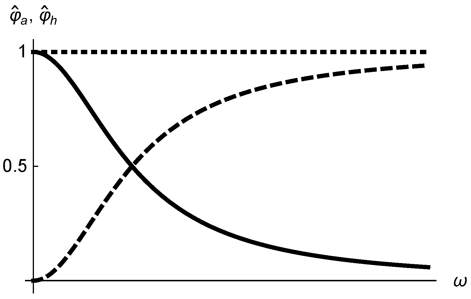An alternative idea [10], further applied in the present work, is to divide the mechanical energy into two components using filter functions. The low-frequency one does not affect the entropy level directly, whereas the high-frequency one is associated with the “heat-like” diffusive energy transfer, causing an entropy increase without a direct contribution to continuum motion.

One more way to correct CTE is to extend constitutive equations. There are two strategies for this: to introduce corrections to (i) Fourier’s law and/or (ii) Duhamel–Neumann law. The majority of theories following the first path (i) result in modified heat equations with a number of new constants that require elaborate and hardly conductible experiments [3]. Namely, the hyperbolic heat conduction equation (Maxwell–Cattaneo) proved itself to be able to be validated only for a limited number of cases [11,12]. For the low-dimensional systems, the approach of discrete thermomechanics [13] provides robust instrumentation in handling heat transfer beyond Maxwell–Cattaneo and Fourier’s laws.

As far as the second path (ii) is concerned, experimental research for two titanium alloys and two aluminium alloys [14,15] has shown that the thermoelastic constant (or coupling parameter, namely $\alpha /\rho c_v$) depends on the sum of principal stresses. In [14,16], an explicit model describing the observed experimental effect [15] is derived based on the fundamental conservation laws for the quasi-static loading. In their next experimental work [17], the authors reported a weak nonlinearity in stress–temperature dependence. Later, a theoretical research of the elastic buckling of columns was made [18], incorporating the results obtained in [16]. This topic keeps being addressed, e.g., in later work [19], the authors revisit the previous analysis, coming to the same conclusions. In [20], it is clearly shown that this theory is able to correctly describe the stress dependence of the photoacoustic signal near a hole in aluminum alloy plates.

In the present work, we combined two approaches, namely, we adopted the nonlinear generalized Duhamel–Neumann law, and then we split the stress into mechanical and “heat-like” parts in order to linearize the set of governing equations. Then, we formulated and solved the boundary value dynamical problem for the obtained system of integro-differential equations, employing the method of eigenfunctions. Finally, we compared the temperature and stress fields to those produced by CTE.

2. CTE with a Modified Thermal Expansion Coefficient

In this section, we derived a nonlinear model of thermoelasticity with regard to the stress-dependent thermal expansion coefficient. Following work [20], let us assume the linear dependence of the thermal coefficient $\tilde{\alpha }$ on the mean stress $\sigma$:

$$\tilde{\alpha }=\alpha +\tilde{\beta }\sigma ,$$

(1)

The coefficient’s $\tilde{\beta }$ value and sign strongly depend on the effects of various physical nature [20,21]. According to the experimental measurements and theoretical predictions [17], it is estimated as $2\times {10}^{-4}{\mathrm{MPa}}^{-1}$.

Next, in order to simplify the analysis of the results without loss of generality, let us restrict ourselves to a purely one-dimensional problem. All of the derivations presented below may be repeated for the 3D theory following [10].

2.1. Equation of Motion

Let us write down the modified Helmholtz free energy density $\rho f$ following [22]:

$$\rho f(e,T)=\frac{1}{2}\left(K+\frac{4}{3}\mu \right)e^2-B\left(e\right)Te-\frac{1}{2}\frac{\rho c_v}{T_0}{T}^2.$$

(2)

Here, e is the strain, T is the deviation from the initial temperature $T_0$, K is the bulk modulus, $\mu$ is the shear modulus, $\rho$ is the material density, and $c_v$ is the specific heat capacity at constant volume. Within CTE, the coefficient B is equal to $\alpha K$, so it is now subject to alteration:

$$B\left(e\right)=(\alpha +\beta e)K.$$

(3)

Here, we introduce this addition to thermal expansion coefficient $\alpha$ being proportional to strain, not stress. The equivalence of the two definitions will be demonstrated below.

Stress is defined as

$$\sigma =\frac{\partial \left(\rho f\right)}{\partial e}=e\left(K(1-2\beta T)+\frac{4}{3}\mu \right)-\alpha KT.$$

(4)

Note that the introduced addition to the thermal expansion coefficient leads to a decrease in the bulk modulus K.

The constitutive Equation (4) is supplemented by the equation of motion and the definition of strain

$${\sigma }^{\prime }=\rho \ddot{u},e=u^{\prime };$$

(5)

therefore, we arrive at the first governing equation:

$$\left(K+\frac{4}{3}\mu \right)u^{″}-\alpha K{T}^{\prime }=\rho \ddot{u}+2\beta K{\left(eT\right)}^{\prime }.$$

(6)

Let us return to the literature-based notation of the addition to the thermal expansion coefficient (1) in order to establish the identity of two approaches.

The generalized Duhamel–Neumann law takes the form

$$\sigma =\left(K+\frac{4}{3}\mu \right)e-\left(\alpha +\tilde{\beta }\sigma \right)KT$$

(7)

Solving it for $\sigma$ gives

$$\sigma =\frac{K+\frac{4}{3}\mu }{1+\tilde{\beta }KT}e-\frac{\alpha K}{1+\tilde{\beta }KT}T$$

(8)

If we restrict ourselves by $\tilde{\beta }KT\ll 1$, the latter becomes

$$\sigma =\left(1-\tilde{\beta }KT\right)\left(K+\frac{4}{3}\mu \right)e-\alpha KT.$$

(9)

If we define

$$\beta =\frac{1}{2}\left(K+\frac{4}{3}\mu \right)\tilde{\beta },$$

(10)

the generalized Duhamel–Neumann law (9) yields to (4).

2.2. Heat Equation

The energy balance and Fourier’s law have the form

$$\rho \dot{U}=\sigma \dot{e}-h^{\prime },h=-\lambda T^{\prime },$$

(11)

where U is the specific internal energy, h is the heat flux, and $\lambda$ is the thermal conductivity coefficient. The balance of the Helmholtz free energy density is written as

$$\rho \dot{f}=\sigma \dot{e}-\eta \dot{T},$$

(12)

where ${\displaystyle \eta =-\frac{\partial \left(\rho f\right)}{\partial T}}$ is the entropy density. In turn, the Helmholtz free energy density is related to the specific internal energy through

$$\rho f=\rho U-T\eta .$$

(13)

Combining the aforesaid, we arrive at the heat equation in the form of

$$T\dot{\eta }=\lambda T^{″}.$$

(14)

Finally, as the entropy density is given by

$$\eta =-\frac{\partial \left(\rho f\right)}{\partial T}=(\alpha +\beta e)Ke+\frac{\rho c_v}{T_0}T,$$

(15)

the second governing equation yields to

$$\alpha KT\dot{e}+2K\beta T\dot{e}e+\frac{\rho c_v}{T_0}T\dot{T}=\lambda T^{″}.$$

(16)

The set of governing equations for CTE with a modified thermal expansion coefficient is given by (6) and (16). For small temperature changes, (16) becomes

$$\alpha K{T}_0\dot{e}+2K\beta T_0\dot{e}e+\rho c_v\dot{T}=\lambda T^{″}.$$

(17)

The resulting system of governing equations is essentially nonlinear. This means that the linearization procedure wipes out the terms containing the parameter $\beta$. Thus, in the next section, we consider an alternative approach.

3. Extended CTE with a Modified Thermal Expansion Coefficient

In order to formulate an extended system of CTE [10], we supplemented the set of differential operators with a convolution operator. The first benefit of this approach is its ability to describe a wider range of physical effects: the filter functions cannot be reduced solely to the derivatives; thus, they add to the model robustness. Secondly, while broadening the applicability range of the model, we remain within the paradigm of linear theories. The filter functions have also proven their relevance in thermoelasticity-related problems. The separate treatment of wave dispersion and acoustic absorption, for example, has been found to be useful in image reconstruction in photoacoustic tomography [23].

3.1. Filter Functions

The convolution of two functions, for instance, $\psi \left(t\right)$ and $\phi \left(t\right)$, was calculated along the entire real axis:

$$\psi \left(t\right)\ast \phi \left(t\right)={\int }_{\mathbb{R}}\psi \left(\tau \right)\phi (t-\tau )dt$$

(18)

In the most general case, a particular solution $\psi \left(t\right)$ is supposed to be obtained as a function defined on the entire real axis $t\in \mathbb{R}$, similar to the filter function $\phi \left(t\right)$.

In the present work, we restricted ourselves to a simplistic filter function having only one parameter $\Omega$, i.e.,

$${\phi }_a\left(t\right)=\sqrt{\frac{\pi }{2}}\Omega e^{-t\Omega },{\widehat{\phi }}_a\left(\omega \right)=\frac{{\Omega }^2}{{\omega }^2+{\Omega }^2}.$$

(19)

The main property of the filter functions, allowing for the lossless splitting procedure, can be written in the frequency domain as

$${\widehat{\phi }}_a\left(\omega \right)+{\widehat{\phi }}_h\left(\omega \right)=1,$$

(20)

where the subscript a stands for the “acoustic” part and subscript h stands for the “heat” part. Figure 1 shows ${\widehat{\phi }}_a$ (solid line) and ${\widehat{\phi }}_h$ (dotted line) as functions of frequency $\omega$; dots indicate the unit level. The graphs intersect at $(\Omega ,0.5)$.

Filters are aimed at satisfying the experimental data on the attenuation of mechanical waves in the medium. A “hat” sign denotes the Fourier transform $\mathfrak{F}\left(\phi \right)=\widehat{\phi }$, and the inverse Fourier transform is ${\mathfrak{F}}^{-1}\left(\widehat{\phi }\right)=\phi$. It is also assumed that the introduced convolutions and Fourier transforms exist at least in the distributional sense. Further details concerning the mathematical apparatus used are available in, e.g., [24,25].

3.2. A Splitting Procedure for Constitutive Equations

The extended CTE system is obtained in [10] within the filter function approach:

$$\begin{array}{c}{\displaystyle \left(K+\frac{4}{3}\mu \right)e^{″}-\alpha K{T}^{″}=\rho {\ddot{e}}_a}\hfill \\ {\displaystyle \rho c_v\dot{T}-\lambda T^{″}+\alpha K{T}_0\dot{e}+\frac{\lambda \rho }{\alpha K}{\ddot{e}}_h=0}\hfill \end{array}$$

(21)

and the Duhamel–Neumann law is written for the acoustic part of the stress only:

$${\sigma }_a=\left(K+\frac{4}{3}\mu \right)e-\alpha KT$$

(22)

Note that (22) is not a plain assumption, but the result of a rigorous derivation by means of the Coleman–Noll procedure.

The system (21) can be rewritten in terms of both stresses and strains:

$$\begin{array}{c}{\displaystyle {\sigma }_a^{″}=\frac{\rho }{K+\frac{4}{3}\mu }\left({\ddot{\sigma }}_a+\alpha K\ddot{T}\right)-\rho {\ddot{e}}_h}\hfill \\ {\displaystyle \left(\rho c_v+\frac{{\alpha }^2{K}^2{T}_0}{K+\frac{4}{3}\mu }\right)\dot{T}=\lambda T^{″}-\frac{\alpha K{T}_0}{K+\frac{4}{3}\mu }{\dot{\sigma }}_a-\frac{\lambda \rho }{\alpha K}{\ddot{e}}_h}\hfill \end{array}$$

(23)

Up to now, we have used all of the possible constitutive equations; therefore, we need to broaden their set. Let us suppose, without contradicting anything previously stated, that

$$\begin{array}{ccccc}{\sigma }_a\hfill & =& {\displaystyle \left(K+\frac{4}{3}\mu \right)e_a}& {\displaystyle +\left(K+\frac{4}{3}\mu \right)e_h}& -\alpha KT\\ {\sigma }_h\hfill & =& 0& -2\beta KT{e}_h& +0\end{array}$$

(24)

Linearization of the last equation gives

$${\sigma }_h=-2\beta K{T}_0{e}_h$$

(25)

Thus, the addition to the stress caused by the addition to the thermal expansion coefficient is equalized to the “filtered” thermal part of the stress ${\sigma }_h$.

Let us note that linearizing the constitutive equation in the conventional manner leads to a trivial result by simply adding up to the bulk modulus

$$\sigma =\left(K+\frac{4}{3}\mu \right)e-\alpha KT-2\beta KeT\approx \left(K(1-2\beta T_0)+\frac{4}{3}\mu \right)e-\alpha KT$$

(26)

Finally, we write the system (21) in terms of stresses only, denoting $\gamma =-2\beta K$

$$\begin{array}{c}{\displaystyle {\sigma }_a^{″}=\frac{\rho }{K+\frac{4}{3}\mu }({\ddot{\sigma }}_a+\alpha K\ddot{T})-\frac{\rho }{\gamma T_0}{\ddot{\sigma }}_h}\hfill \\ {\displaystyle \left(\rho c_v+\frac{{\alpha }^2{K}^2{T}_0}{K+\frac{4}{3}\mu }\right)\dot{T}=\lambda T^{″}-\frac{\alpha K{T}_0}{K+\frac{4}{3}\mu }{\dot{\sigma }}_a-\frac{\lambda \rho }{\alpha K\gamma T_0}{\ddot{\sigma }}_h}\hfill \end{array}$$

(27)

Note that parameter $\beta$ (or $\gamma$) being responsible for the nonlinearity in Equations (6) and (16) appears here in linear terms. That is to say, adopting such an approach, we obtain the second time derivative of a dependent variable in the heat equation, correcting only the mechanical part (i.e., Duhamel–Neumann law).

3.3. Limiting Cases

Firstly, putting thermal expansion coefficient $\alpha$ to 0 uncouples the system of equations, returning the d’Alembert wave equation for $\sigma$ and the classical heat equation for T. Secondly, choosing a filter function so that ${\sigma }_a=\sigma$ and ${\sigma }_h=0$ converts (27) to the CTE system. Thirdly, if the whole “mechanical” spectrum goes to the thermal part, i.e., ${\sigma }_a=0$ and ${\sigma }_h=\sigma$, the system (27) results in the well-known Maxwell–Cattaneo hyperbolic heat equation

$$\rho c_v^{\ast }(\tau \ddot{T}+\dot{T})-\lambda T^{″}=0,$$

(28)

where ${\displaystyle \rho c_v^{\ast }=\rho c_v+\frac{{\alpha }^2{K}^2{T}_0}{(K+\frac{4}{3}\mu )}}$, ${\displaystyle \tau =\frac{\lambda }{c_v^{\ast }(K+\frac{4}{3}\mu )}}$. Therefore, the propagation speed of thermal disturbance (also referred to as “second sound”) would be equal to the speed of sound in the medium, namely ${\displaystyle c_h=\sqrt{\frac{K+\frac{4}{3}\mu }{\rho }}}$.

4. Solution to the Extended CTE Boundary Value Problem with a Modified Thermal Expansion Coefficient

Let us consider a boundary value problem for an infinite semi-opaque thermally insulated slab of thickness $x\in [0,l]$. It is irradiated by a short laser pulse hitting its surface $x=0$. The interaction of laser irradiation and the slab is modeled by the internal heat sources distributed over the volume. The Lambert–Beer law, also known as the Bouguer law, governs light extinction in a semi-opaque medium:

$$I=I_0{e}^{-{\gamma }_{0}x},$$

(29)

where $I_0$ is the intensity of light flux entering the layer, and the extinction coefficient ${\gamma }_0$ is determined by the wavelength of the laser and the physical properties of the medium itself. The skin-layer $1/{\gamma }_0$ is much narrower than the width of the slab l. Thus, the heat sources distributed over the volume are concentrated near the irradiated boundary.

The set of Equation (27) yields to

$$\begin{array}{c}{\sigma }_a^{″}=a_1{\ddot{\sigma }}_a+a_2\ddot{T}-a_3{\ddot{\sigma }}_h\hfill \\ T^{″}=b_1{\dot{\sigma }}_a+b_2\dot{T}-b_3{\ddot{\sigma }}_h+b_4{e}^{-{\gamma }_{0}x}\delta \left(t\right),\hfill \end{array}$$

(30)

where $\delta \left(t\right)$ is the Dirac delta function and

$$\begin{array}{cccc}{\displaystyle a_1=\frac{\rho }{K+\frac{4}{3}\mu },}\hfill & {\displaystyle a_2=\frac{\alpha K\rho }{K+\frac{4}{3}\mu },}\hfill & {\displaystyle a_3=\frac{\rho }{\gamma T_0}}\hfill & \\ {\displaystyle b_1=\frac{\alpha K{T}_0}{\lambda (K+\frac{4}{3}\mu )},}\hfill & {\displaystyle b_2=\frac{\rho c_v}{\lambda }+\frac{{\alpha }^2{K}^2{T}_0}{\lambda (K+\frac{4}{3}\mu )},}\hfill & {\displaystyle b_3=\frac{\rho }{\alpha K\gamma T_0},}\hfill & {\displaystyle b_4=\frac{\rho I_0}{\lambda },}\hfill \end{array}$$

(31)

along with homogeneous boundary and initial conditions

$$\begin{array}{cccc}\sigma {\mid }_{x=0}=0,\hfill & T^{\prime }{\mid }_{x=0}=0,\hfill & \sigma {\mid }_{x=l}=0,\hfill & T^{\prime }{\mid }_{x=l}=0,\hfill \\ \sigma {\mid }_{t=0}=0,\hfill & T{\mid }_{t=0}=0,\hfill & \dot{\sigma }{\mid }_{t=0}=0,\hfill & \dot{T}{\mid }_{t=0}=0.\hfill \end{array}$$

(32)

In order to obtain the solution, we need to convert the system of partial differential Equation (30) to an algebraic system using integral transforms. We multiplied the matrix of the system (30) by the column of eigenfunctions and integrated it over the interval $[0,l]$, performing the so-called finite integral transform with respect to the coordinate. Then, we took the Laplace transform with respect to time. After the respective inverse transforms [26,27], we arrived at the formal series

$$T(x,t)=\frac{1}{l}{T}_0+\frac{2}{l}\sum _{n=1}^{\infty }{T}_{n}cos\left(x\sqrt{{\lambda }_n}\right);\sigma (x,t)=\frac{2}{l}\sum _{n=1}^{\infty }{\sigma }_{n}sin\left(x\sqrt{{\lambda }_n}\right),$$

(33)

where ${\lambda }_n={\pi }^2{n}^2/l^2$ and ${\sigma }_n$, $T_n$ are given by

$$\begin{array}{c}{\displaystyle T_n=\frac{a_3{Q}_n}{a_2{b}_3}\sum _{i=1}^6\left(\frac{e^{t{R}_i}(a_3{R}_i^4-a_1{\Omega }^2{R}_i^2-{\lambda }_n^2{\Omega }^2)}{{\displaystyle \prod _{j=1,..,6}^{j\ne i}}(R_i-R_j)}\right),}\hfill \\ {\displaystyle {\sigma }_n=-\frac{Q_n}{b_3}\sum _{i=1}^6\left(\frac{e^{t{R}_i}{R}_i^2}{{\displaystyle \prod _{j=1,..,6}^{j\ne i}}(R_i-R_j)}\right),}\hfill \\ {\displaystyle Q_n=\frac{b_4{\gamma }_0{l}^2\left(1+{(-1)}^{n+1}{e}^{-{\gamma }_{0}l}\right)}{{\gamma }_0^2{l}^2+{\pi }^2{n}^2}}\hfill \end{array}$$

(34)

and

$$\begin{array}{c}{\displaystyle T_0=-\frac{b_4\left(1-e^{-l{\gamma }_0}\right)}{a_2{b}_3(a_2{b}_1-a_1{b}_2){\gamma }_0{\displaystyle \prod _{j=1,..,3}^{j\ne i}}(r_i-r_j)}\left(3a_1{\Omega }^2(a_2{b}_1-a_1{b}_2)-2a_1{a}_2{b}_3\left(r_3{r}_1^2+r_2^2{r}_1+r_2{r}_3^2\right)+\right.}\hfill \\ +a_2{e}^{r_{2}t}\left(a_1{b}_3{r}_2^2(r_1-r_3)-a_3{b}_1(r_1+2r_2)r_3\right)-a_2{r}_3{e}^{r_{3}t}(r_1-r_2)(a_1{b}_3{r}_3+a_3{b}_1)+\hfill \\ \left.+e^{r_{1}t}\left(3a_1^2{b}_2{\Omega }^2+a_1{a}_2\left(b_3\left(2r_3{r}_1^2+\left(r_2^2+r_3^2\right)r_1+r_2{r}_3(r_2+r_3)\right)-3b_1{\Omega }^2\right)+a_2{a}_3{b}_1(2r_1+r_2)r_3\right)\right)\hfill \end{array}$$

(35)

Here, $R_i$ is the roots of the sixth-order equation

$$a_2{b}_3{R}^6+a_3{b}_2{R}^5+a_3{\lambda }_n^2{R}^4+(a_2{b}_1-a_1{b}_2){\Omega }^2{R}^3-a_1{\lambda }_n^2{\Omega }^2{R}^2-b_2{\lambda }_n^2{\Omega }^{2}R-{\lambda }_n^4{\Omega }^2=0$$

(36)

and $r_i$ is the non-zero roots of the respective third-order equation if ${\lambda }_n=0$:

$$a_2{b}_3{r}^3+a_3{b}_2{r}^2+(a_2{b}_1-a_1{b}_2){\Omega }^2=0$$

(37)

We would like to draw the readers’ attention to the fact that the solution to (36) has three more roots in addition to the CTE solution [27]. These roots generate auxiliary dispersion curves, driving the wave propagation process. In the next section, we will demonstrate their impact.

5. Discussion

The solution (33) obtained in the form of a series consists of two parts: the first part includes classical roots $R_1$, $R_2$, and $R_3$ in the numerator, which we will refer to as the “classical part”; the second “non-classical part” includes roots $R_4$, $R_5$, and $R_6$, which vanish if we set parameter $\beta =0$ and/or choose ${\widehat{\phi }}_a=1$ and ${\widehat{\phi }}_h=0$. The final form of the solution depends on how the amplitudes of the classical and non-classical components of the solution are related to the characteristic times and coordinate scales of each of them. Typical stress, temperature, and displacement fields are analyzed below.

Let us begin with a series of figures that illustrate the evolution of temperature and stress fields, namely, Figure 2 and Figure 3a,c show the solution (33), while Figure 3b,d demonstrate the same boundary value problem treated within CTE.

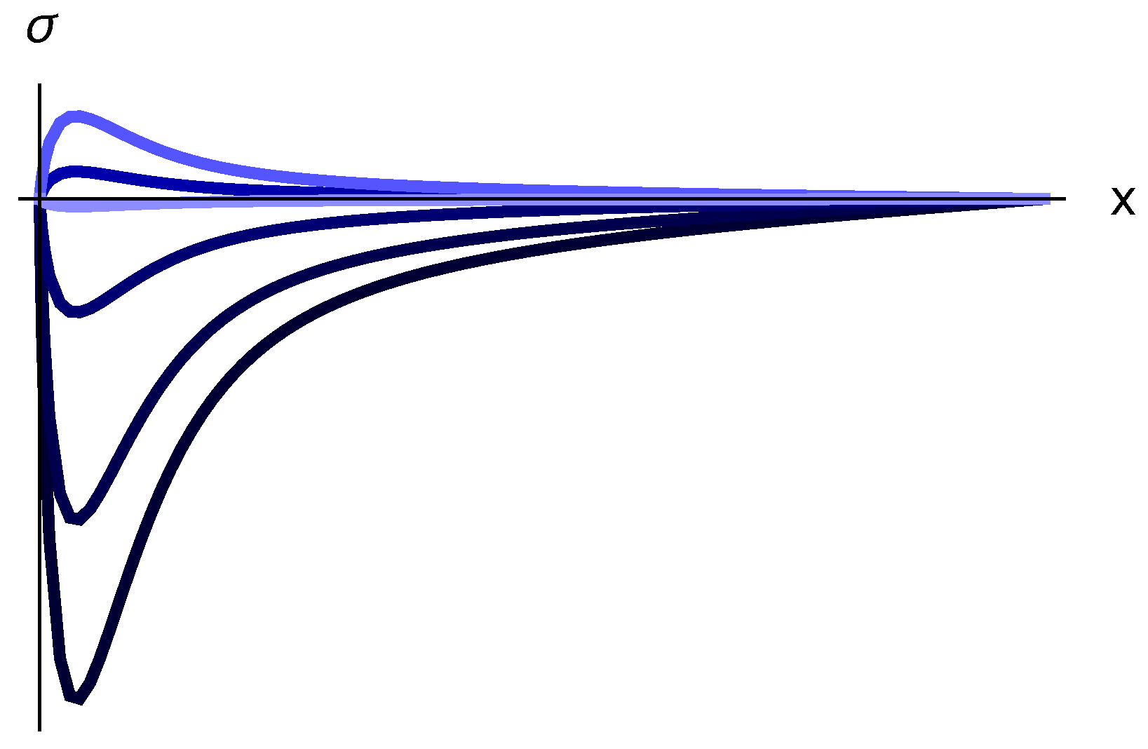
The component of the solution, corresponding to the “classical” roots (Figure 2), attenuates rapidly over the time typical for the CTE model. At larger times, this component contributes insignificantly to the amplitude of the slower processes of mechanical waves absorption modeled with the filter function (20).

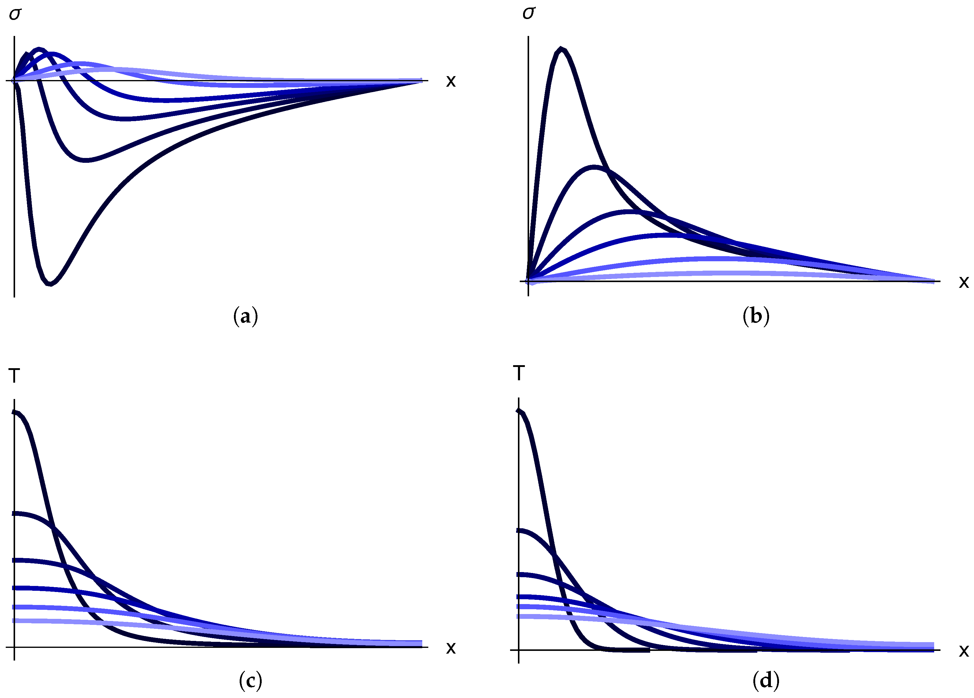
The behavior of the solution component, which is determined by the part of the series with non-classical roots, is illustrated in Figure 3a. This dependence, at certain times, has two extrema and areas in which stress takes both negative and positive values. Figure 3b shows the stress fields obtained within CTE. There is only one extremum, which can be either positive or negative, depending on the sign of the thermal expansion coefficient $\alpha$. Thus, unlike the solution (33), the classical solution cannot change the sign with time or have two extrema.

Figure 3c,d show the time slices for the non-stationary temperature field in the layer of thickness l, for the extended CTE with a modified thermal expansion coefficient (33), and for the CTE, respectively. There are no fundamental differences in the temperature plots; however, in CTE, the transition to the equilibrium state takes less time.

A separate analysis of the displacement field was carried out. The solution (33) was substituted into the equation of dynamics (5) and integrated twice with respect to time. The respective initial conditions were set as homogeneous.

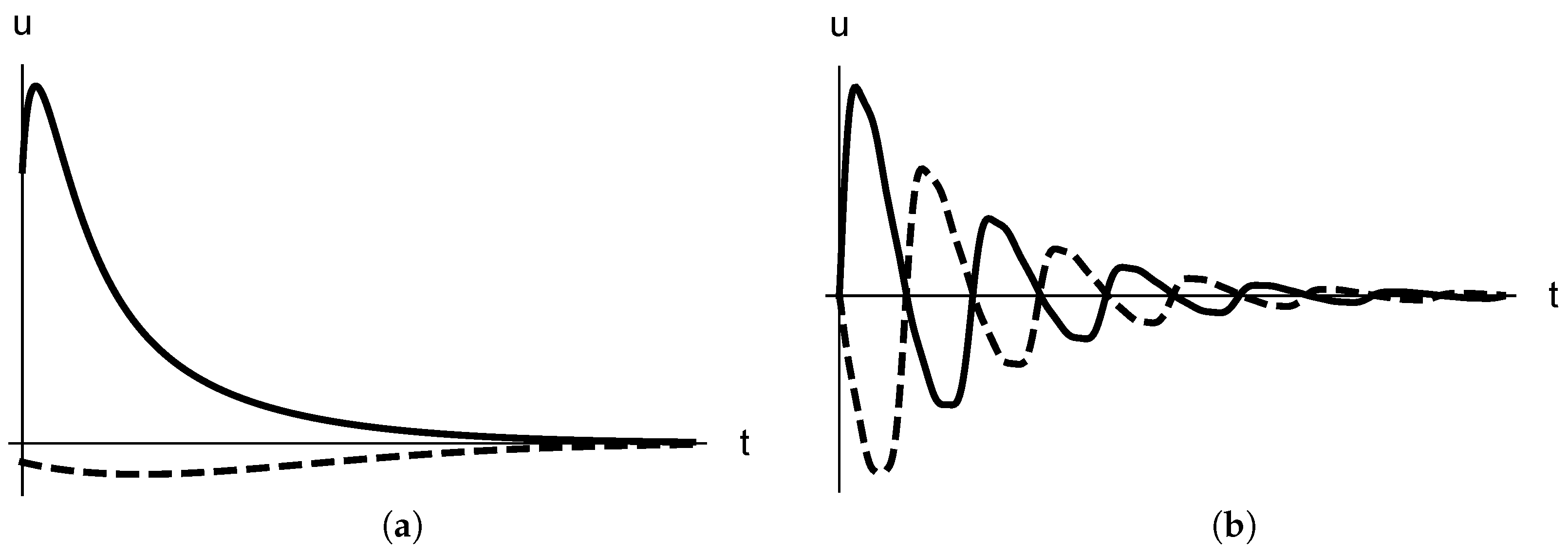
The initial fast expansion of the layer (the “first phase”) is shown in Figure 4a as a jump associated with the classical thermoelastic effect [22]. The sample reaches its maximum thickness in the slower second expansion phase, which takes place due to the absorption of mechanical waves modeled by the filter function (20). Depending on the choice of thermomechanical parameters, each of the phases can contribute more or less significantly to the final displacement of the layer boundaries. Figure 4b shows the respective results for CTE: an oscillatory process with a relatively high frequency, which is achieved by the small thermal expansion coefficient $\alpha$, the small layer thickness l, and the high speed of sound in the medium.

We would like to note that, in classical thermoelasticity (CTE), the acoustic wave consists of only two components: quasi-acoustic and quasi-thermal ones. Their behavior is described by the corresponding branches of the dispersion curves. The laser pulse modeled by the volumetrically distributed heat sources directly generates only the quasi-thermal component of the acoustic wave, whereas the quasi-acoustic component appears due to the coupling effect.

In the extended theory, the acoustic wave turns out to have three components. In the problem considered, the quasi-thermal component is an expansion wave. In view of the absence of mechanical action on the layer in the problem statement, the second, quasi-acoustic component does not make a substantial contribution. The third component becomes noticeable somewhat later, when its amplitude reaches the values comparable to the first component. According to the parameters chosen, this component is a compression wave, thus correcting the first wave component in amplitude (approximately, as it would have been carried out by a nonlinear term), which can be seen in Figure 3a. One of the possible physical interpretations of these phenomena is a system of two nested sublattices; they have different feedback times and thermal expansion coefficients, so one of them starts expanding with a noticeable lag.

What is more, the greater the parameter $\beta$, the more prominent the local minimum of stresses becomes in the vicinity of the irradiated boundary. This effect is also due to the third wave process prescribed by the model. Its behavior is governed by the additional curve in the phonon spectrum, which is the subject of further investigation. A separate analysis has shown that the conventional speed of sound is the only asymptotic available in the system.

6. Conclusions

To sum everything up, we proposed a novel approach to the extension of classical thermoelasticity, which incorporated the experimentally observed nonlinearity in the thermal expansion coefficient and remained within the framework of linear models. By tuning the filter function, we can customize the frequency dependence of the attenuation coefficient to satisfy the experimental data. This model can be successfully applied to describe media with a microstructure that undergoes structural changes during the passage of mechanical waves, as well as internal friction. Detailed studies of the associated effects, the phonon spectrum, and the extension to 3D are subjects of further investigation.

Comparing the extended CTE with a modified thermal expansion coefficient to the CTE itself, we conclude that it gives almost no differences in the behavior of the temperature curves, but provides a number of significant alterations in stress fields. Namely, we prove that the model allows us to meet the experiments in which two extrema are simultaneously observed for the stress-over-time-dependence. The similarity between the enhanced theory and CTE is that both models adopt classical Fourier’s law. This means that the heat equation is parabolic in both cases, i.e., the so-called “heat front” is absent in the solution, unless we consider a limiting case (28).

References

1. Chandrasekharaiah, D.S. Hyperbolic thermoelasticity: A review of recent literature. Appl. Mech. Rev. 1998, 51, 705–729. [Google Scholar] [CrossRef]
2. Müller, I.; Müller, W.H. Fundamentals of Thermodynamics and Applications: With Historical Annotations and Many Citations from Avogadro to Zermelo; Springer: Berlin, Germany, 2009. [Google Scholar]
3. Jou, D.; Casas-Vazquez, J.; Lebon, G. Extended Irreversible Thermodynamics; Springer: Berlin, Germany, 2010. [Google Scholar]
4. Ignaczak, J.; Ostoja-Starzewski, M. Thermoelasticity with Finite Wave Speeds; Oxford University Press: New York, NY, USA, 2010. [Google Scholar]
5. Mashinskii, E. Amplitude-frequency dependencies of wave attenuation in single-crystal quartz: Experimental study. J. Geophys. Res. 2008, 113, B11304. [Google Scholar] [CrossRef]
6. Chang, C.W.; Okawa, D.; Garcia, H.; Majumdar, A.; Zettl, A. Breakdown of Fourier’s law in nanotube thermal conductors. Phys. Rev. Lett. 2008, 101, 075903. [Google Scholar] [CrossRef] [PubMed] [Green Version]
7. Johnson, J.A.; Maznev, A.A.; Cuffe, J.; Eliason, J.K.; Minnich, A.J.; Kehoe, T.; Sotomayor Torres, C.M.; Chen, G.; Nelson, K.A. Direct measurement of room-temperature nondiffusive thermal transport over micron distances in a silicon membrane. Phys. Rev. Lett. 2013, 110, 025901. [Google Scholar] [CrossRef] [PubMed] [Green Version]
8. Vovnenko, N.V.; Zimin, B.A.; Sudenkov, Y.V. Experimental study of thermoelastic stresses in heat-conducting and non-heat-conducting solids under submicrosecond laser heating. Tech. Phys. 2011, 56, 803–808. [Google Scholar] [CrossRef]
9. Povstenko, Y. Fractional Thermoelasticity; Springer: Cham, Switzerland, 2015. [Google Scholar]
10. Babenkov, M.B. A model of the thermoelastic medium absorbing a part of the acoustic spectrum. Contin. Mech. Thermodyn. 2021, 33, 789–802. [Google Scholar] [CrossRef]
11. Peshkov, V.P. Second sound in helium II. Sov. Phys. JETP 1960, 11, 580–584. [Google Scholar]
12. Poletkin, K.V.; Gurzadyan, G.G.; Shang, J.; Kulish, V. Ultrafast heat transfer on nanoscale in thin gold films. Appl. Phys. B 2012, 107, 137–143. [Google Scholar] [CrossRef]
13. Podolskaya, E.A.; Krivtsov, A.M.; Kuzkin, V.A. Discrete thermomechanics: From thermal echo to ballistic resonance (a review). In Mechanics and Control of Solids and Structures; Polyanskiy, V.A., Belyaev, A.K., Eds.; Springer: Cham, Switzerland, 2022; pp. 501–533. [Google Scholar]
14. Rosenfield, A.R.; Averbach, B.L. Effect of stress on the expansion coefficient. J. Appl. Phys. 1956, 27, 154–156. [Google Scholar] [CrossRef]
15. Machin, A.S.; Sparrow, J.G.; Stimson, M.G. Mean stress dependence of the thermoelastic constant. Strain 1987, 23, 27–30. [Google Scholar] [CrossRef]
16. Wong, A.K.; Jones, R.; Sparrow, J.G. Thermoelastic constant or thermoelastic parameter? J. Phys. Chem. Solids 1987, 48, 749–753. [Google Scholar] [CrossRef]
17. Wong, A.K.; Sparrow, J.G.; Dunn, S.A. On the revised theory of the thermoelastic effect. J. Phys. Chem. Solids 1988, 49, 395–400. [Google Scholar] [CrossRef]
18. Bert, C.W.; Fu, C. Implications of stress dependency of the thermal expansion coefficient on thermal buckling. J. Press. Vessel Technol. 1992, 114, 189–192. [Google Scholar] [CrossRef]
19. Le, Q.X.; Torero, J.L.; Dao, V.T. Understanding the effects of stress on the coefficient of thermal expansion. Int. J. Eng. Sci. 2019, 141, 83–94. [Google Scholar] [CrossRef]
20. Glazov, A.L.; Morozov, N.F.; Muratikov, K.L. Theoretical and experimental investigation of a laser-induced photoacoustic effect near a hole in internally stressed metal plates. Phys. Mesomech. 2020, 23, 213–222. [Google Scholar] [CrossRef]
21. Morozov, N.F.; Muratikov, K.L.; Indeitsev, D.A.; Vavilov, D.S.; Semenov, B.N. A new model of the electron gas effect on the thermoacoustics of conductors under laser irradiation. Phys. Mesomech. 2019, 22, 13–17. [Google Scholar] [CrossRef]
22. Nowacki, W. Dynamic Problems of Thermoelasticity; Springer: Dordrecht, The Netherlands, 1975. [Google Scholar]
23. Treeby, B.E.; Zhang, E.Z.; Cox, B.T. Photoacoustic tomography in absorbing acoustic media using time reversal. Inverse Probl. 2010, 26, 115003. [Google Scholar] [CrossRef]
24. Pervozvansky, A.A. Theory Course of the Automatic Control; Nauka: Moscow, Russia, 1986. [Google Scholar]
25. Smith, C.A.; Corripio, A.B. Principles and Practice of Automatic Process Control, 2nd ed.; Wiley: New York, NY, USA, 1997. [Google Scholar]
26. Lebedev, N.N.; Skalskaya, I.P.; Ulflyand, Y.S. Worked Problems in Applied Matematics; Dover Publications: New York, NY, USA, 1979; pp. 103–142. [Google Scholar]
27. Vitokhin, E.Y.; Babenkov, M.B. Numerical and analytical study of the propagation of thermoelastic waves in a medium with heat-flux relaxation. J. Appl. Mech. Tech. Phys. 2016, 57, 537–549. [Google Scholar] [CrossRef]
Figure 1. Filter functions φ ^ a (solid) and φ ^ h (dashed).
Mathematics 10 04142 g001
Figure 2. Evolution of the “classical” part of the non-stationary stress field, which corresponds to the roots R 1 , R 2 , and R 3 in the solution (33). The colormap goes from dark to light over time.
Mathematics 10 04142 g002
Figure 3. Evolution of stress (a,b) and temperature (c,d) fields. Colormap goes from dark to light over time. Plots (a,c) illustrate the solution (33), plots (b,d) correspond to the solution obtained within CTE.
Mathematics 10 04142 g003
Figure 4. Displacements of the irradiated boundary x = 0 (solid) and the opposite boundary x = l (dashed), calculated within (a) the proposed solution (33) and (b) CTE.
Mathematics 10 04142 g004
Publisher’s Note: MDPI stays neutral with regard to jurisdictional claims in published maps and institutional affiliations.