
An Adapted Discrete Lindley Model Emanating from Negative Binomial Mixtures for Autoregressive Counts


Abstract
:1. Introduction
1.1. The Lindley Distribution as Departure Point
1.2. Lindley Counting Models: INAR and Other Cases
1.3. Contributions and Foci of This Paper
- A (continuous) noncentral Lindley type II (i.e., ncLII) distribution is systematically constructed, and statistical characteristics are derived;
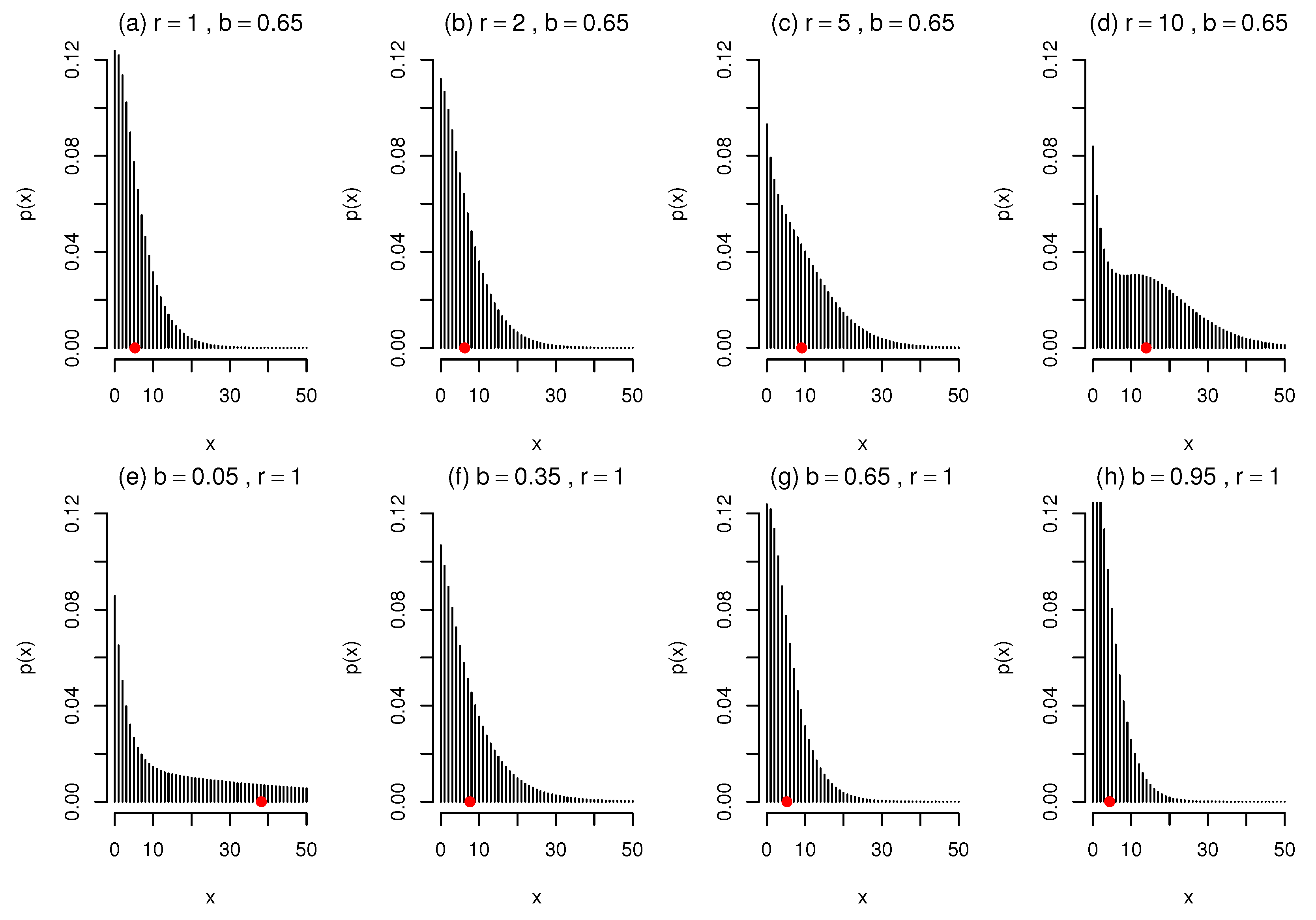
- A (discrete) counting model based on this noncentral Lindley type II distribution is derived via compounding with the Poisson distribution (i.e., PncLII), together with essential statistical characteristics;
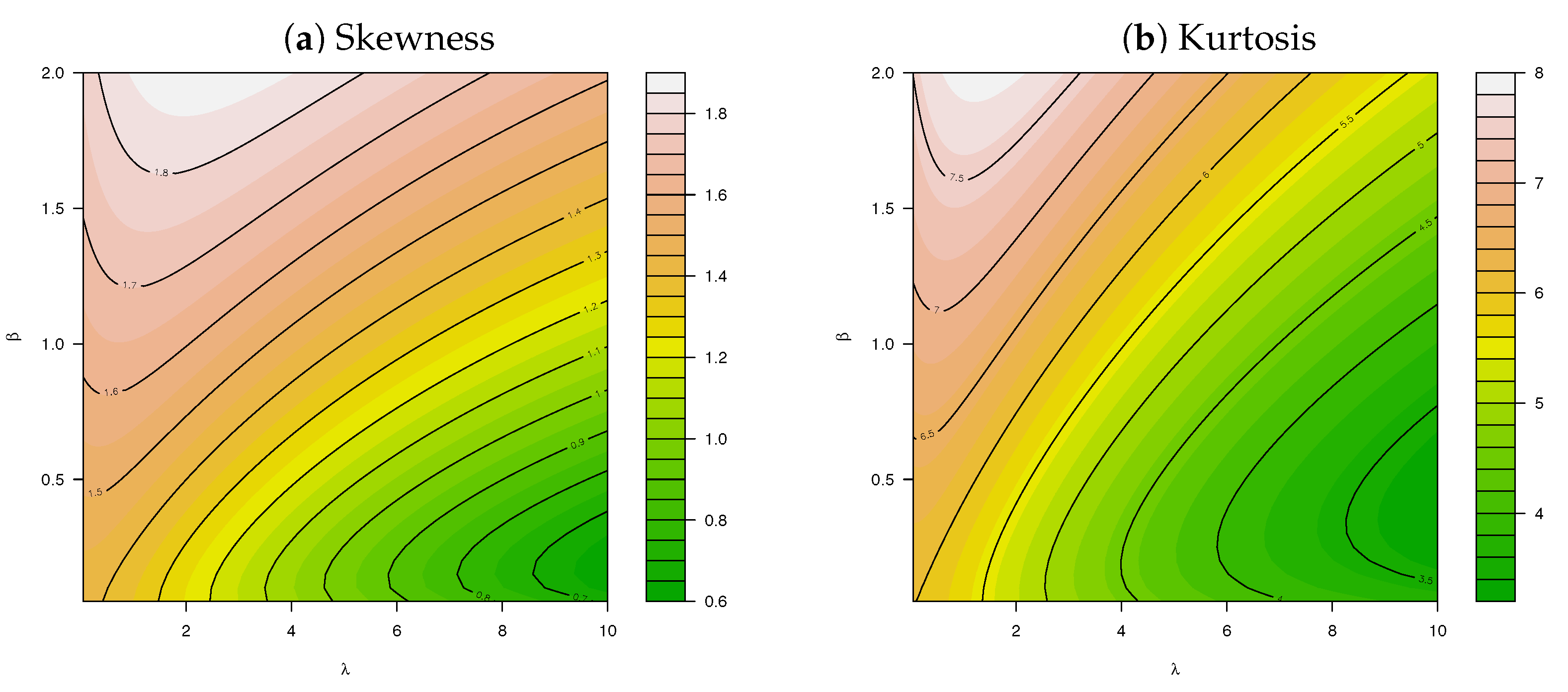
- Key insights are attained through investigation of the skewness, kurtosis, and the DI compared to the work of [6]; and finally,
- This discrete counting model is implemented and illustrated as an error structure (i.e., ) within an INAR(1) environment and juxtaposed against the PncLI for the error structures in a simulation study and real data applications.
2. Construction


3. Implementation
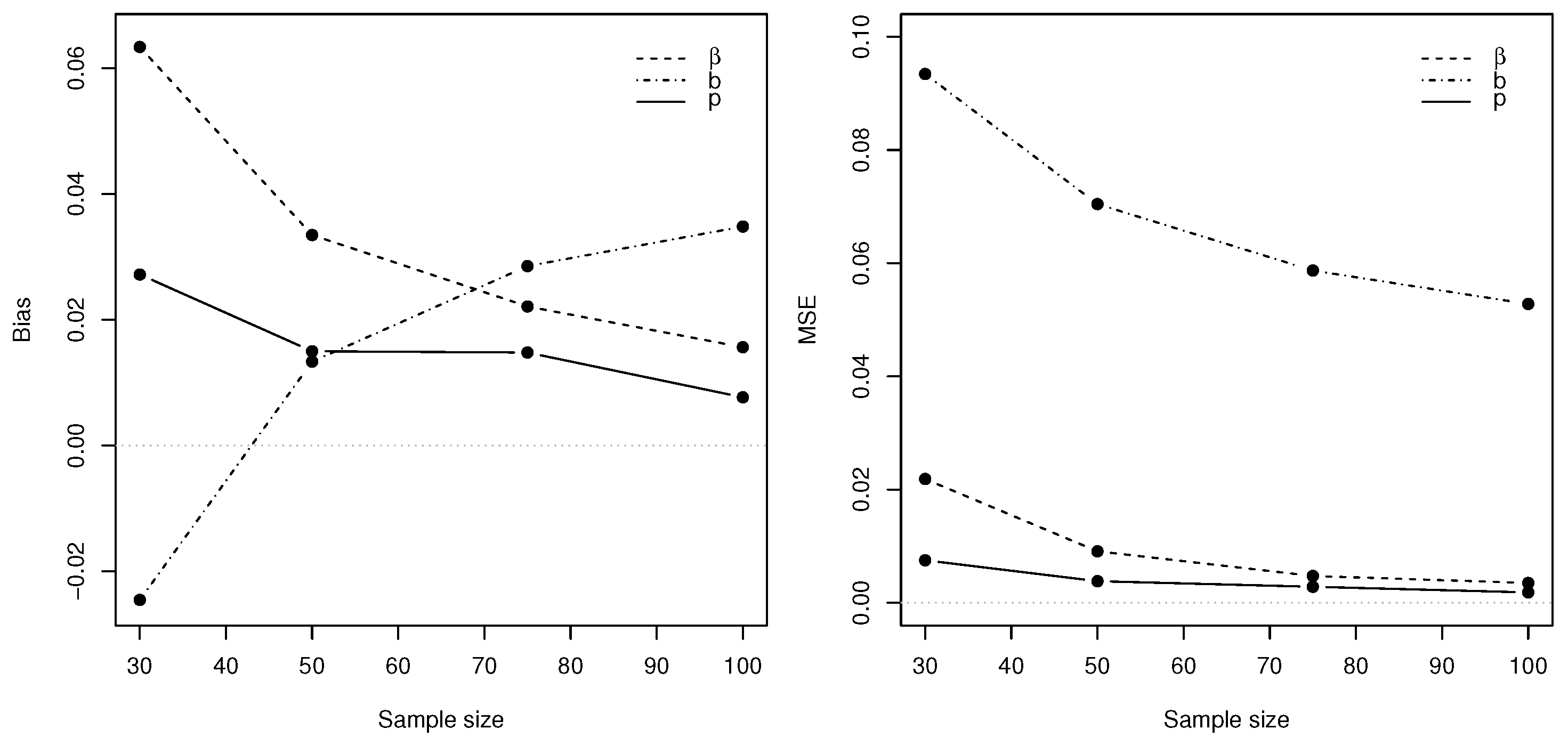
3.1. Simulation
- Define the theoretical parameters , , , and , and set the simulation replication number equal to 500.
- Generate errors for sample sizes such that with .
- (a)
- Generate variates.
- (b)
- Generate the errors such that .
- Generate the time series with binomial variates such that
- Because the stationary marginal distribution of is not explicitly available, a burn-in period should be generated, of which the corresponding marginal distributions then converge to the desired stationary marginal distribution [34]; in this case, we initialise .
- In order to estimate under various sample sizes, the conditional log-likelihood function (16) is maximised using the optim() function in .
- The bias and mean squared error (MSE) are calculated for each of the estimators for the different sample sizes of T, where

3.2. Real-Data Applications
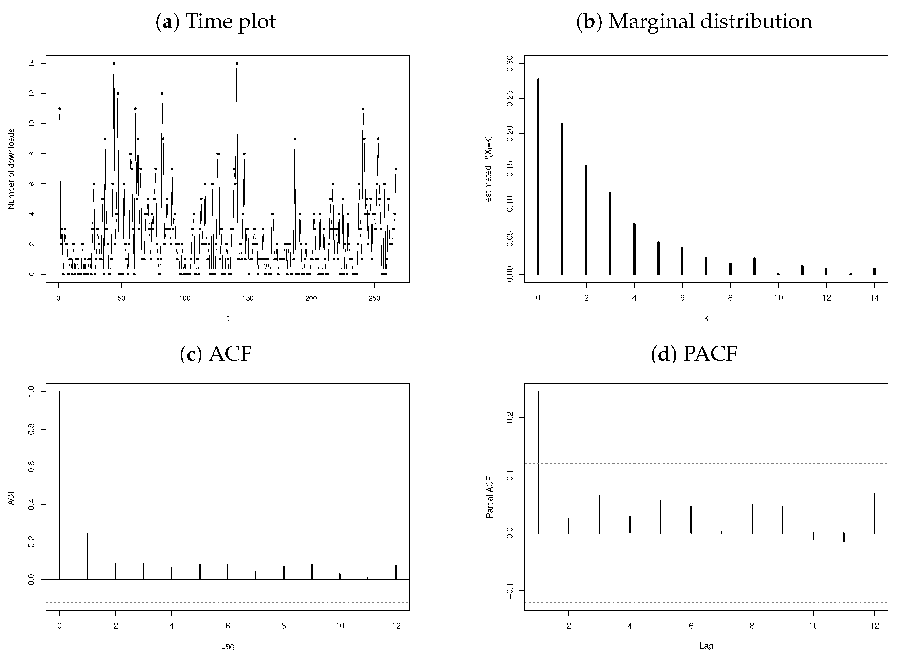
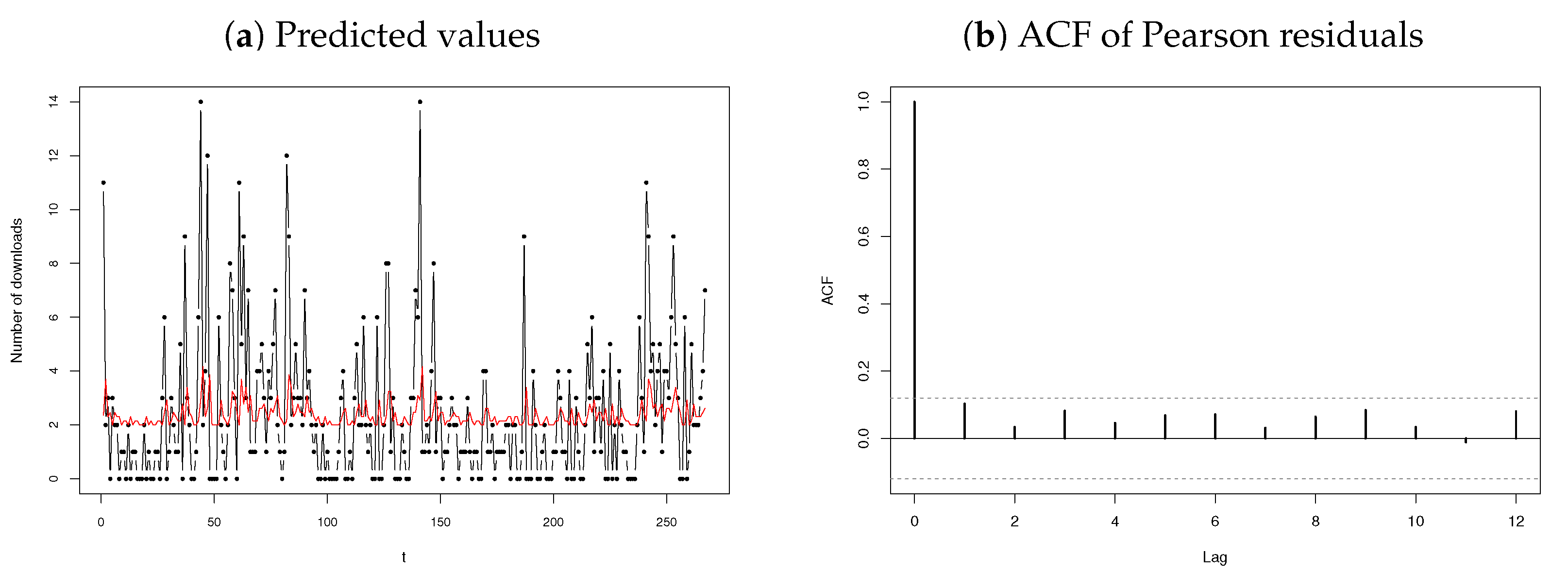
- Daily number of downloads of certain software for the period from June 2006 to February 2007 (sample size ) [36].
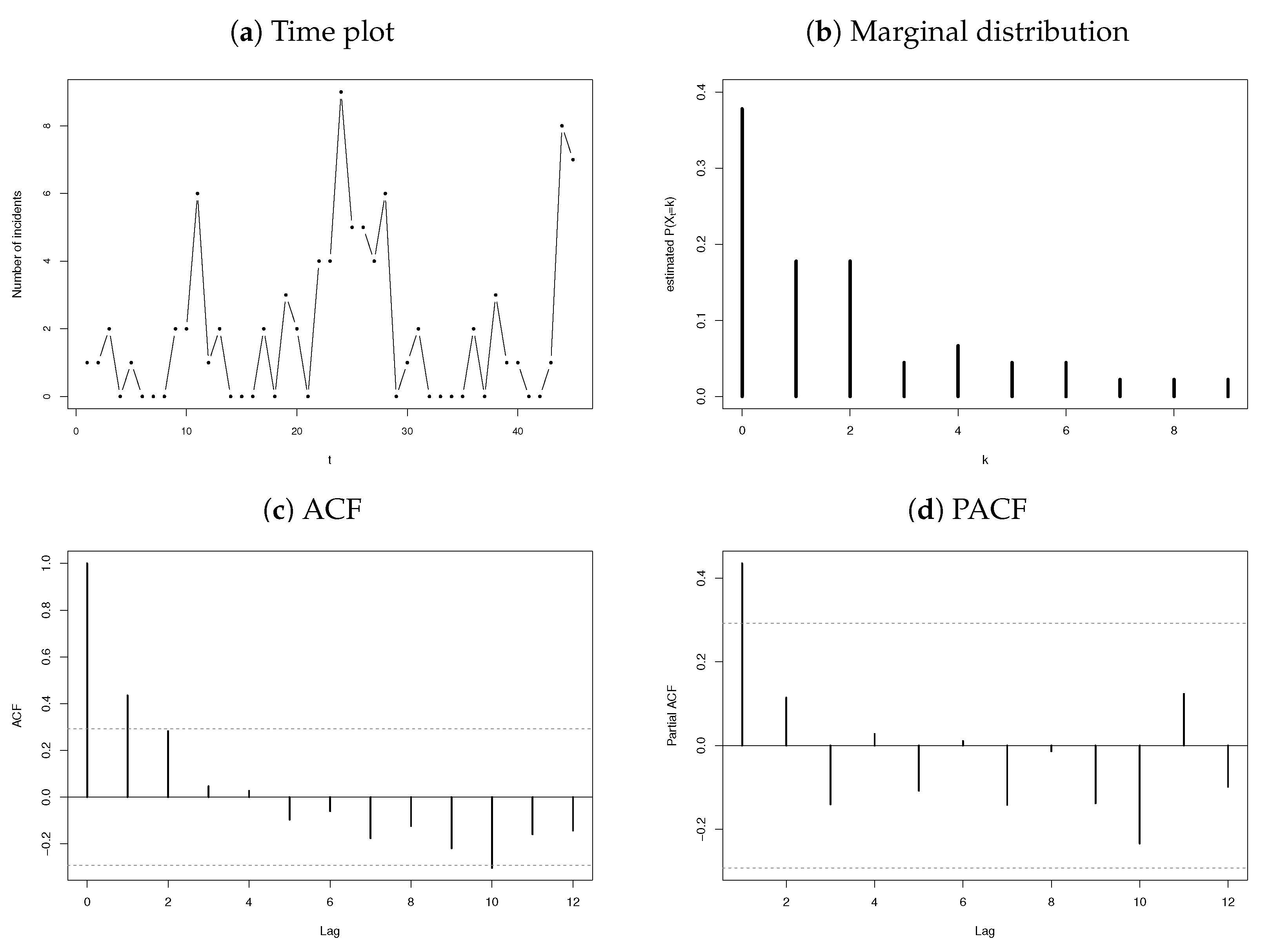
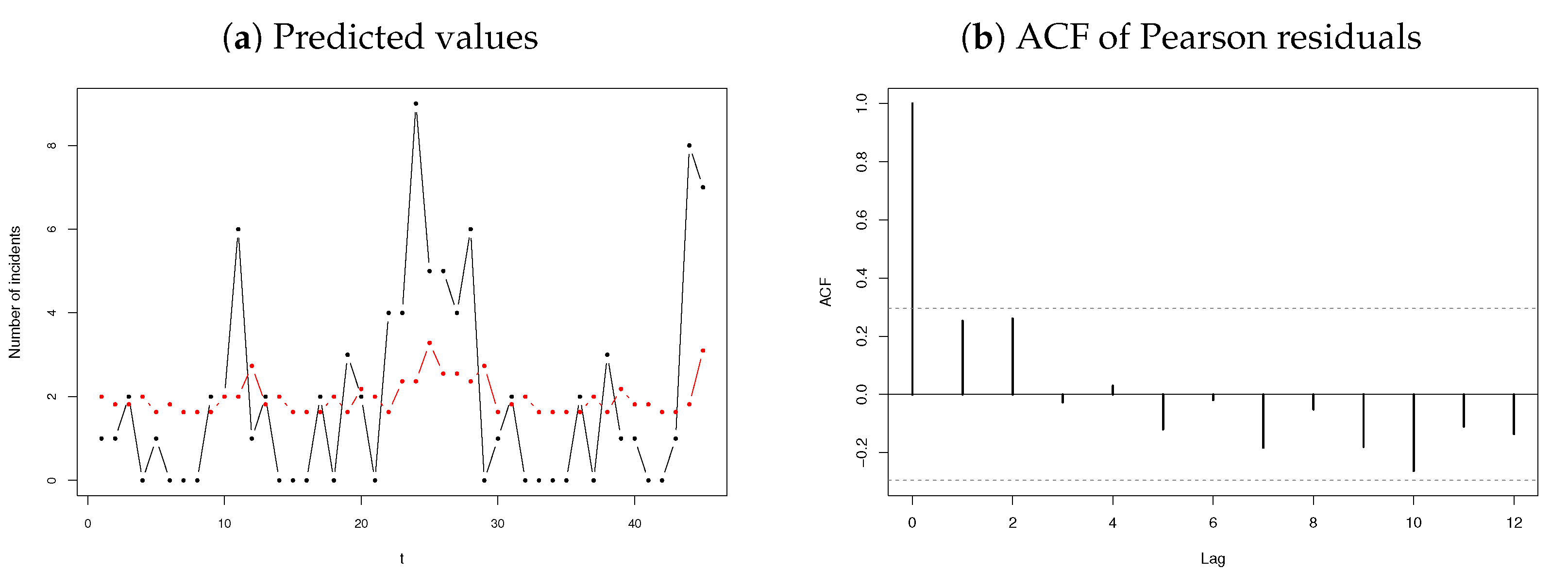
- Yearly number of terrorism incidents in Australia for years 1970 to 2015 (sample size ). The data are available in the Ecdat package of software.
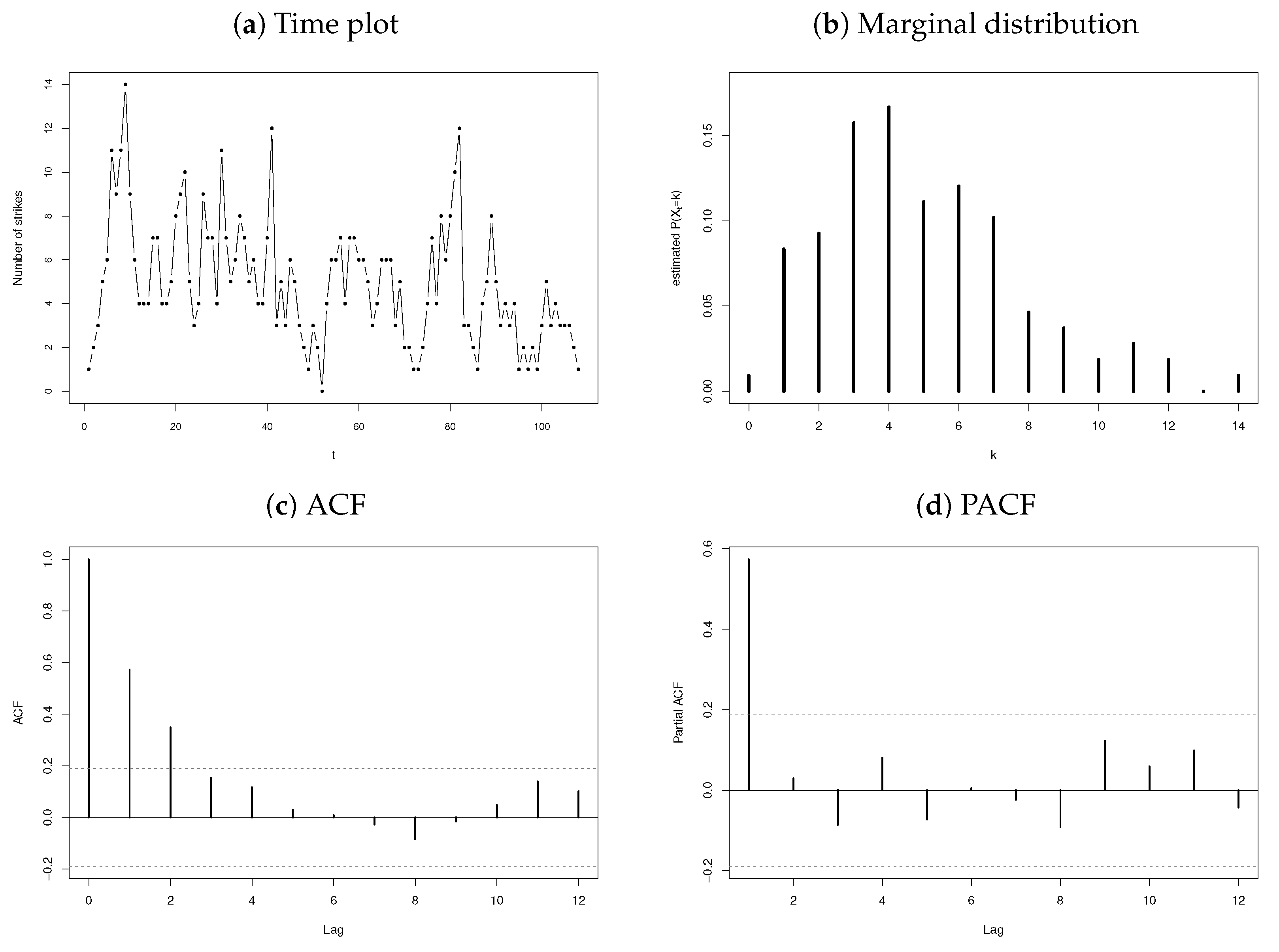
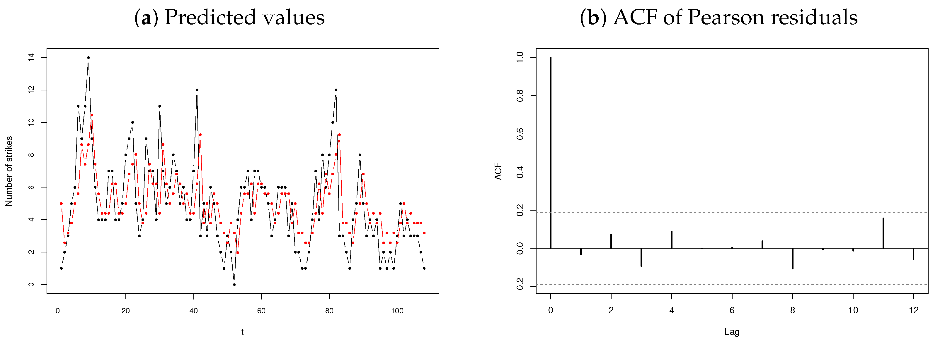
- Monthly number of strikes leading to at least 1000 workers being idle (published by the U.S. Bureau of Labor Statistics, http://www.bls.gov/wsp/, accessed on 1 December 2021). The time period from January 1994 to December 2002 (sample size ) is considered.
3.2.1. Number of Downloads of Certain Software


3.2.2. Number of Terrorism Incidents


3.2.3. Number of Strikes


3.3. Discussion
4. Conclusions
Author Contributions
Funding
Institutional Review Board Statement
Informed Consent Statement
Data Availability Statement
Acknowledgments
Conflicts of Interest
Abbreviations
| Exp | Exponential |
| Gam | Gamma |
| Bin | Binomial |
| ncLI | noncentral Lindley of type I |
| ncLII | noncentral Lindley of type II |
| PncLI | Poisson noncentral Lindley of type I |
| PncLII | Poisson noncentral Lindley of type II |
| DI | Dispersion index |
| NB | Negative binomial |
| INAR | Integer autoregressive |
| MGF | Moment-generating function |
| MSE | Mean squared error |
| PGF | Probability-generating function |
| ACF | Autocorrelation function |
| PACF | Partial autocorrelation function |
| AIC | Akaike’s information criterion |
Appendix A. Moments of the Noncentral Lindley of Type II
Appendix B. Moments of the Noncentral Lindley of Type I

Appendix C. Moments of the Poisson Noncentral Lindley of Type I

References
- Lindley, D.V. Fiducial distributions and Bayes’ theorem. J. R. Stat. Soc. Ser. B (Methodol.) 1958, 20, 102–107. [Google Scholar] [CrossRef]
- Ghitany, M.E.; Atieh, B.; Nadarajah, S. Lindley distribution and its application. Math. Comput. Simul. 2008, 78, 493–506. [Google Scholar] [CrossRef]
- Zakerzadeh, H.; Dolati, A. Generalized Lindley distribution. J. Math. Ext. 2009, 3, 13–25. [Google Scholar]
- Ghitany, M.; Al-Mutairi, D.K.; Balakrishnan, N.; Al-Enezi, L. Power Lindley distribution and associated inference. Comput. Stat. Data Anal. 2013, 64, 20–33. [Google Scholar] [CrossRef]
- Shanker, R.; Shukla, K.K.; Shanker, R.; Tekie, A. A three-parameter Lindley distribution. Am. J. Math. Stat. 2017, 7, 15–26. [Google Scholar]
- Ferreira, J.; van der Merwe, A. A Noncentral Lindley Construction Illustrated in an INAR (1) Environment. Stats 2022, 5, 70–88. [Google Scholar] [CrossRef]
- Knüsel, L.; Bablok, B. Computation of the noncentral gamma distribution. SIAM J. Sci. Comput. 1996, 17, 1224–1231. [Google Scholar] [CrossRef]
- Nadarajah, S.; Kotz, S. Compound mixed Poisson distributions I. Scand. Actuar. J. 2006, 2006, 141–162. [Google Scholar] [CrossRef]
- Nadarajah, S.; Kotz, S. Compound mixed Poisson distributions II. Scand. Actuar. J. 2006, 2006, 163–181. [Google Scholar] [CrossRef]
- Ferreira, J.; Bekker, A.; Arashi, M. Bivariate noncentral distributions: An approach via the compounding method. S. Afr. Stat. J. 2016, 50, 103–122. [Google Scholar] [CrossRef]
- Sankaran, M. The discrete Poisson-Lindley distribution. Biometrics 1970, 26, 145–149. [Google Scholar] [CrossRef]
- Ghitany, M.; Al-Mutairi, D. Estimation methods for the discrete Poisson–Lindley distribution. J. Stat. Comput. Simul. 2009, 79, 1–9. [Google Scholar] [CrossRef]
- Mahmoudi, E.; Zakerzadeh, H. Generalized poisson–Lindley distribution. Commun. Stat. Methods 2010, 39, 1785–1798. [Google Scholar] [CrossRef]
- Das, K.K.; Ahmad, J.; Bhattacharjee, S. A new three-parameter Poisson-Lindley distribution for modeling over dispersed count data. Int. J. Appl. Eng. Res. 2018, 13, 16468–16477. [Google Scholar]
- Altun, E. A new two-parameter discrete Poisson-generalized Lindley distribution with properties and applications to healthcare data sets. Comput. Stat. 2021, 36, 2841–2861. [Google Scholar] [CrossRef]
- Lívio, T.; Khan, N.M.; Bourguignon, M.; Bakouch, H.S. An INAR (1) model with Poisson–Lindley innovations. Econ. Bull. 2018, 38, 1505–1513. [Google Scholar]
- McKenzie, E. Some simple models for discrete variate time series. Water Resour. Bull. 1985, 21, 645–650. [Google Scholar] [CrossRef]
- Al-Osh, M.A.; Alzaid, A.A. First-order integer-valued autoregressive (INAR (1)) process. J. Time Ser. Anal. 1987, 8, 261–275. [Google Scholar] [CrossRef]
- Altun, E. A new generalization of geometric distribution with properties and applications. Commun. Stat.-Simul. Comput. 2020, 49, 793–807. [Google Scholar] [CrossRef]
- Altun, E. A new one-parameter discrete distribution with associated regression and integer-valued autoregressive models. Math. Slovaca 2020, 70, 979–994. [Google Scholar] [CrossRef]
- Abd-Elrahman, A.M. Utilizing ordered statistics in lifetime distributions production: A new lifetime distribution and applications. J. Probab. Stat. Sci. 2013, 11, 153–164. [Google Scholar]
- Altun, E.; Bhati, D.; Khan, N.M. A new approach to model the counts of earthquakes: INARPQX (1) process. SN Appl. Sci. 2021, 3, 1–17. [Google Scholar] [CrossRef] [PubMed]
- Bhati, D.; Kumawat, P.; Gómez-Déniz, E. A new count model generated from mixed Poisson transmuted exponential family with an application to health care data. Commun. Stat.-Theory Methods 2017, 46, 11060–11076. [Google Scholar] [CrossRef]
- Altun, E.; Khan, N.M. Modelling with the novel INAR (1)-PTE process. Methodol. Comput. Appl. Probab. 2022, 24, 1735–1751. [Google Scholar] [CrossRef]
- Xavier, D.; Santos-Neto, M.; Bourguignon, M.; Tomazella, V. Zero-Modified Poisson-Lindley distribution with applications in zero-inflated and zero-deflated count data. arXiv 2017, arXiv:1712.04088. [Google Scholar]
- Sharafi, M.; Sajjadnia, Z.; Zamani, A. A first-order integer-valued autoregressive process with zero-modified Poisson-Lindley distributed innovations. Commun. Stat.-Simul. Comput. 2020. [Google Scholar] [CrossRef]
- Zhang, J.; Zhu, F.; Khan, N.M. A new INAR model based on Poisson-BE2 innovations. Commun. Stat.-Theory Methods 2022. [Google Scholar] [CrossRef]
- Habibi, M.; Asgharzadeh, A. A new mixed Poisson distribution: Modeling and applications. J. Test. Eval. 2018, 46, 1728–1740. [Google Scholar] [CrossRef]
- Altun, E.; Cordeiro, G.M.; Ristić, M.M. An one-parameter compounding discrete distribution. J. Appl. Stat. 2022, 49, 1935–1956. [Google Scholar] [CrossRef]
- Simon, L.J. The negative binomial and Poisson distributions compared. Proc. Casualty Actuar. Soc. 1960, 47, 20–24. [Google Scholar]
- R Core Team. R: A Language and Environment for Statistical Computing; R Foundation for Statistical Computing: Vienna, Austria, 2022. [Google Scholar]
- Bain, L.J.; Engelhardt, M. Introduction to Probability and Mathematical Statistics; Duxbury Press: Belmont, CA, USA, 1992; Volume 4. [Google Scholar]
- Gradshteyn, I.S.; Ryzhik, I.M. Table of Integrals, Series, and Products; Academic Press: Cambridge, MA, USA, 2014. [Google Scholar]
- Weiß, C.H. An Introduction to Discrete-Valued Time Series; John Wiley & Sons: Hoboken, NJ, USA, 2018. [Google Scholar]
- Alzaid, A.; Al-Osh, M. First-order integer-valued autoregressive (INAR (1)) process: Distributional and regression properties. Stat. Neerl. 1988, 42, 53–61. [Google Scholar] [CrossRef]
- Weiß, C.H. Thinning operations for modeling time series of counts—a survey. AStA Adv. Stat. Anal. 2008, 92, 319–341. [Google Scholar] [CrossRef]
- Akaike, H. A new look at the statistical model identification. IEEE Trans. Autom. Control 1974, 19, 716–723. [Google Scholar] [CrossRef]
- Neethling, A.; Ferreira, J.; Bekker, A.; Naderi, M. Skew generalized normal innovations for the AR(p) process endorsing asymmetry. Symmetry 2020, 12, 1253. [Google Scholar] [CrossRef]

| Model | Parameter | Estimate | AIC | Mean () | Variance () | |
|---|---|---|---|---|---|---|
| INAR-P(1) | p | 0.1718 | 634.1 | 1272.2 | 2.3655 | 2.3655 |
| (0.0323) | ||||||
| 1.9590 | ||||||
| (0.1096) | ||||||
| INAR-NB(1) | p | 0.1544 | 537.9 | 1081.7 | 2.3657 | 7.1888 |
| (0.0415) | ||||||
| r | 0.8501 | |||||
| (0.1491) | ||||||
| b | 0.2982 | |||||
| (0.0373) | ||||||
| INAR-PL(1) | p | 0.1180 | 541.1 | 1086.1 | 2.3559 | 5.5808 |
| (0.0400) | ||||||
| 0.7554 | ||||||
| (0.0527) | ||||||
| INAR-PncLI(1) | p | 0.1573 | 537.9 | 1081.7 | 2.3700 | 6.6734 |
| (0.0415) | ||||||
| 1.3054 | ||||||
| (0.2414) | ||||||
| 5.4097 | ||||||
| (2.5779) | ||||||
| INAR-PncLII(1) (for ) | p | 0.1515 | 537.9 | 1081.8 | 2.3659 | 7.2181 |
| (0.0407) | ||||||
| 1.1080 | ||||||
| (0.1583) | ||||||
| b | 0.3875 | |||||
| (0.1071) | ||||||
| INAR-PncLII(1) (for ) | p | 0.1554 | 537.7 | 1081.4 | 2.3656 | 7.0867 |
| (0.0409) | ||||||
| 1.1957 | ||||||
| (0.1898) | ||||||
| b | 0.4938 | |||||
| (0.1122) | ||||||
| INAR-PncLII(1) (for ) | p | 0.1577 | 537.7 | 1081.4 | 2.3667 | 6.9021 |
| (0.0411) | ||||||
| 1.2680 | ||||||
| (0.2190) | ||||||
| b | 0.6698 | |||||
| (0.1009) | ||||||
| INAR-PncLII(1) (for ) | p | 0.1579 | 537.7 | 1081.5 | 2.3676 | 6.8009 |
| (0.0413) | ||||||
| 1.2908 | ||||||
| (0.2306) | ||||||
| b | 0.7934 | |||||
| (0.0761) |
| Model | Parameter | Estimate | AIC | Mean () | Variance () | |
|---|---|---|---|---|---|---|
| INAR-P(1) | p | 0.3085 | 93.6 | 191.3 | 2.0379 | 2.0379 |
| (0.0851) | ||||||
| 1.4093 | ||||||
| (0.2182) | ||||||
| INAR-NB(1) | p | 0.1969 | 82.4 | 170.8 | 2.0107 | 5.6309 |
| (0.1358) | ||||||
| r | 0.7494 | |||||
| (0.3135) | ||||||
| b | 0.3170 | |||||
| (0.1027) | ||||||
| INAR-PL(1) | p | 0.1950 | 83.0 | 170.1 | 1.9986 | 4.0675 |
| (0.1282) | ||||||
| 0.9417 | ||||||
| (0.1813) | ||||||
| INAR-PncLI(1) | p | 0.1800 | 82.2 | 170.4 | 1.9976 | 5.3266 |
| (0.1440) | ||||||
| 1.6410 | ||||||
| (0.5842) | ||||||
| 6.9169 | ||||||
| (5.9401) | ||||||
| INAR-PncLII(1) for | p | 0.1966 | 82.6 | 171.1 | 2.0110 | 5.3104 |
| (0.1354) | ||||||
| 1.3010 | ||||||
| (0.4396) | ||||||
| b | 0.3946 | |||||
| (0.2767) | ||||||
| INAR-PncLII(1) (for ) | p | 0.1923 | 82.4 | 170.9 | 2.0073 | 5.3783 |
| (0.1384) | ||||||
| 1.4186 | ||||||
| (0.5011) | ||||||
| b | 0.4827 | |||||
| (0.2593) | ||||||
| INAR-PncLII(1) (for ) | p | 0.1865 | 82.3 | 170.6 | 2.0023 | 5.3794 |
| (0.1414) | ||||||
| 1.5347 | ||||||
| (0.5514) | ||||||
| b | 0.6409 | |||||
| (0.2172) | ||||||
| INAR-PncLII(1) (for ) | p | 0.1836 | 82.2 | 170.5 | 1.9998 | 5.3615 |
| (0.1427) | ||||||
| 1.5855 | ||||||
| (0.5689) | ||||||
| b | 0.7629 | |||||
| (0.1634) |
| Model | Parameter | Estimate | AIC | Mean () | Variance () | |
|---|---|---|---|---|---|---|
| INAR-P(1) | p | 0.5061 | 234.5 | 473.1 | 4.9810 | 4.9810 |
| (0.0560) | ||||||
| 2.4600 | ||||||
| (0.2988) | ||||||
| INAR-NB(1) | p | 0.5484 | 231.8 | 469.7 | 4.9810 | 6.8575 |
| (0.0579) | ||||||
| r | 3.8567 | |||||
| (2.4028) | ||||||
| b | 0.6316 | |||||
| (0.1339) | ||||||
| INAR-PL(1) | p | 0.6062 | 234.0 | 471.9 | 5.0017 | 9.5604 |
| (0.0414) | ||||||
| 0.7912 | ||||||
| (0.0966) | ||||||
| INAR-PncLI(1) | p | 0.6062 | 234.0 | 473.9 | 4.9999 | 9.5560 |
| (0.0414) | ||||||
| 0.7914 | ||||||
| (0.0967) | ||||||
| 0.000002 | ||||||
| (0.00002) | ||||||
| INAR-PncLII(1) (for ) | p | 0.6061 | 234.0 | 473.9 | 5.0019 | 9.5621 |
| (0.0419) | ||||||
| 0.7910 | ||||||
| (0.1587) | ||||||
| b | ≈ 1.0000 | |||||
| (0.4764) |
Publisher’s Note: MDPI stays neutral with regard to jurisdictional claims in published maps and institutional affiliations. |
© 2022 by the authors. Licensee MDPI, Basel, Switzerland. This article is an open access article distributed under the terms and conditions of the Creative Commons Attribution (CC BY) license (https://creativecommons.org/licenses/by/4.0/).
Share and Cite
van der Merwe, A.; Ferreira, J.T. An Adapted Discrete Lindley Model Emanating from Negative Binomial Mixtures for Autoregressive Counts. Mathematics 2022, 10, 4141. https://doi.org/10.3390/math10214141
van der Merwe A, Ferreira JT. An Adapted Discrete Lindley Model Emanating from Negative Binomial Mixtures for Autoregressive Counts. Mathematics. 2022; 10(21):4141. https://doi.org/10.3390/math10214141
Chicago/Turabian Stylevan der Merwe, Ané, and Johannes T. Ferreira. 2022. "An Adapted Discrete Lindley Model Emanating from Negative Binomial Mixtures for Autoregressive Counts" Mathematics 10, no. 21: 4141. https://doi.org/10.3390/math10214141