Numerical Method for System Level Simulation of Long-Distance Pneumatic Conveying Pipelines

Abstract

Pneumatic conveying pipelines (PCPs) provide an effective manner for long-distance transport of capsules because of their advantages in high speed, superior safety, and full automation. For better development of PCPs, a system-level simulation tool is desired, but not yet available. In this work, a new 1D model describing systemic dynamics of airflow and capsule movement in PCPs is presented, and 3D simulation is proposed to obtain the characteristic coefficients in the 1D model. The complete model accounts for those phenomena that most profoundly affect the performance of PCPs, such as the 3D layout of the pipeline, the geometry of capsules, as well as the compressibility of air in a long pipeline. A finite volume method is also presented to numerically calculate the model equations, and thereby realize the successful system-level simulation of practical PCPs for the first time. Experimental data were used for validation. For a 550 m-long and small-diameter (27.86 mm) PCP, the errors of predicted conveying times were within 4.43%. For another 30 m-long and large-diameter (125.6 mm) PCP, the errors of predicted conveying time and maximum capsule velocity were within 1%. By enabling readily and accurate prediction of the conveying process, the method provides a feasible tool for the design and application of PCP systems.

1. Introduction

Transportation of capsules through pipelines has been extensively used in various industries. These capsules are typically hollow containers filled with minerals [1], radioactive materials [2], waste [3,4], or other goods [5,6,7,8]. As air is readily available, pneumatic capsule pipelines (PCPs) has drawn substantial attention and have been successfully used in mineral industries, tunnel construction, waste disposal facility and hospitals [2,3,4,5,6,7,9,10,11,12,13,14,15,16,17]. Recently, efforts have been paid to develop a high-speed transport system with pneumatic pipelines [10]. Superior characteristics of PCPs have been exhibited, such as high speed, ecological safety, simple structure, handy operation, and the possibility to fully automate the movement [5,6,7,8,9,10]. Especially for hazardous chemicals or radioactive waste, PCPs provide an effective way to non-contact transportation that avoids most of the potential risks [2].

The performance of a PCP system depends on a series of parameters, such as the size and architecture of the pipeline, the geometry of capsules, the operation pressure, and so on [18,19]. Numerical simulation provides an important and powerful tool for the research and development of PCPs [19,20]. By predicting the performance of a new PCP system at the early stage, optimal design can be more easily achieved, and the development cost can also be significantly reduced.

Currently, there has been a lot of research work focused on developing a numerical method for the pneumatic conveying of granular materials [21,22,23,24,25,26,27]. One of the commonly used approaches is the Eulerian/Lagrangian method, where particles are tracked in a Lagrangian frame of reference either individually or as groups with identical properties [28,29]. An alternative approach has been computational fluid dynamics (CFD), with two-fluid continuum models to represent the gas and solid phases as two interpenetrating continua [23,30]. Further, the technique of particle dynamics simulation has also been widely used for investigations of granular and gas-solid systems. In particular, the discrete element method (DEM), has been successfully applied [31]. Several research workers have also applied the approach of combining DEM with CFD [21,25,26].

Despite success in simulating pneumatic conveying of granular materials, the aforementioned methods are not applicable to PCPs, where the solid size is comparable to the feature size of flow and thus their geometry of capsules has a significant impact on the conveying process. Detailed prediction of capsule motion requires the accurate computation of the fluid-structure interaction (FSI), which means fluid forces acting on solid as well as the impact of solid motion on fluid flow need to be calculated simultaneously [32,33,34]. In a similar situation, i.e., investigation on hydraulic capsule pipelines (HCPs) often involves CFD simulation where both solid and fluid regions are modeled in detail and dynamic mesh/moving mesh techniques are involved to predict the 6 degrees of freedom motion of capsules [35,36,37,38,39]. Such techniques help people to obtain insight into the local processes in PCPs/HCPs, but face big problems when they are used for system-level simulation. The dynamic meshing algorithm will face a serious challenge to maintain mesh validity and quality in case of large-scale motion of capsules, particularly for the pipelines in PCPs that are often as long as several hundred or even thousands of meters [5,9,10]. Moreover, pitching motion may occur and then there will be intensive interaction the between capsule and pipe wall. It is going to be extremely difficult, if not impossible, to directly simulate the overall process with 3D CFD techniques.

A lot of efforts have been made to establish simplified methods to predict the overall performance of PCPs. In the 1980s, Akira and Katsuya derived 1D formulas to describe the pressure loss characteristics of concentric and eccentric capsule pipelines [13,14,15]. Morikawa et al. established an analytical model based on a series of fundamental experiments, and the characteristics of capsule motion during accelerating and decelerating were analyzed. Tomita simulated capsule movement in a section of a pneumatic pipeline based on a 1D model and the pattern of capsule collision was discussed [20]. Latterly, Kosugi et al. utilized a similar 1D model to evaluate the capsule acceleration and energy consumption characteristics of PCPs [1,2,9,12]. York and Liu derived a theoretical model to predict the drag coefficients of pneumatic capsules [11]. These models played very important roles in the development of industrial PCPs. However, the incompressible flow assumption implied in the models is likely to deviate from the fact significantly for long-distance pipelines. Moreover, the models were all established based on oversimplified pipeline architecture (a single horizontal/vertical tube), although practical PCPs are often composed of multiple horizontal, vertical, and bend segments in which forces applied on capsules may vary a lot. In addition, the pressure difference on both ends of the capsule was considered the only aerodynamic force in the models, which means the viscosity force was neglected [7]. Such an assumption may be correct in case the capsules have regular shapes and are constructed with end plates [8]. Nevertheless, for capsules that have complicated aerodynamic configurations [16], the viscosity force may play an important role in capsule conveying. As a result, the currently available methods are still insufficient to perform accurate system level simulation for practical PCPs. A more effective simulation tool is still desired to support people in determining the optimal design parameters and operation conditions.

In this work, a novel method is presented to evaluate the system-level performance of PCPs with practical pipeline layout, capsule geometry and operating conditions. The method utilizes synergistic simulation based on a new 1D model describing the systemic behavior in cooperation with conventional 3D CFD models reflecting local characteristics. The models are established as simply as possible but still account for those phenomena that most profoundly affect the performance of PCPs. The method has been validated with practical PCPs, and favorable accuracy has been demonstrated. By readily and accurately predicting the overall performance of a PCP, the method provides an effective tool for the early-stage design of pneumatic conveying systems.

2. Mathematical Model

2.1. Air Flow

As mentioned above, the airflow in a PCP tends to be highly unsteady and chaotic, and moreover, the axial dimension is often extremely large relative to the sectional dimensions. Precise modeling and simulation of the three-dimensional flow field in the whole pipeline is practically impossible and unnecessary. Instead, the dynamic distribution of air pressure and flow rate along the pipeline axis i often of greater interest [40]. Therefore, a one-dimensional flow model is established to describe the system-level behaviors in PCPs in this work.

For a one-dimensional transient flow, the continuum equation is given by [41]

$$\frac{\partial \rho }{\partial t}+\frac{1}{A}\frac{\partial Q}{\partial x}=0$$

(1)

where ρ is the air density, t is time, A is the pipeline cross-sectional area, Q is the mass flow rate of air, and x is the location along the pipeline, respectively.

According to the ideal gas law, along with the hypothesis of the isothermal process, the equation can be modified as

$$\frac{1}{RT}\frac{\partial p}{\partial t}+\frac{1}{A}\frac{\partial Q}{\partial x}=0$$

(2)

where p denotes the absolute pressure, R is the gas constant (287.053 m²/s²/K for dry air) and T is the absolute temperature of air.

Based on Equation (2), together with a momentum equation, p and Q in a PCP could be determined. For the ease of calculation, an explicit form of momentum equation, like the Hagen-Poiseuille equation, would be preferred. However, there is no such equation available corresponding to the turbulent and compressible flow in PCPs. In this study, a simplified manner is proposed. A series of 3D CFD simulations with regard to typical kinds of pipeline segments (straight/bend and with/without capsules) is proposed to be performed in advance, and then model order reduction based on data fitting can be performed to obtain the desired explicit form equation. It has been found that second-order polynomials shown below can be used with favorable goodness of fit.

$$\frac{\partial p}{\partial x}=k_1{Q}^2+k_{2}Q$$

(3)

where k₁ and k₂ are the fitting coefficients to be determined according to 3D simulation. A previous study also demonstrated such a simple formula is precious enough to describe the flow characteristic of pneumatic pipe with capsules [8]. Based on Equation (3), the axial gradient of flowrate in Equation (2) can be derived as

$$\frac{\partial Q}{\partial x}=\frac{1}{2k_{1}Q+k_2}\frac{\partial }{\partial x}(\frac{\partial p}{\partial x})$$

(4)

Substituting Equation (4) into Equation (2), a governing equation describing the dynamic pressure of airflow in PCPs is obtained.

$$\frac{\partial p}{\partial t}+\mathsf{\Gamma }\frac{\partial }{\partial x}(\frac{\partial p}{\partial x})=0$$

(5)

Similar governing equations in parabolic form have already been used in modeling long-distance gas pipelines where air compressibility needs to be taken into account [41,42]. In the current study, the coefficient Γ is given by

$$\mathsf{\Gamma }=\frac{RT}{A(2k_{1}Q+k_2)}$$

(6)

2.2. Capsule Movement

A capsule may be subjected to various forces in PCPs, as shown in Figure 1. Among those forces, the pressure difference on both ends of the capsule usually acts as a main driving force, which can be determined according to the calculated air pressure profile [11,18]

$$F_p=Ac·\mathsf{\Delta }p$$

(7)

where F_p is the net pressure force acting on a capsule, A_c is the area of capsule end and Δp is the pressure difference.

Whatever the configuration and location of the capsule are, there is always a certain gap between the capsule and the pipe wall. When air flows through the gap, a viscous force, F_v, will be produced on the surface of the capsule and provide additional driving or drag force for the capsule. Such force highly depends on the shape of the capsule as well as the relative movement between the capsule and air flow. To account for such an effect in a simple manner, curve-fitting based on three-dimensional CFD simulation is also used. Correspondingly, another second-order polynomial will be obtained, that is,

$$F_v=k_3{Q}_l^2+k_4{Q}_l$$

(8)

where Q_l is the flow rate of air that flows across the capsule surface (i.e., leakage flow rate), and k₃ and k₄ are the fitting coefficients, respectively.

During the movement of the capsule, the friction force, F_f, between the capsule and the pipe wall acts as a resistance force. It can be evaluated as follows [18]:

$$F_f=-fG$$

(9)

where f is the sliding friction coefficient, and G is the capsule weight.

In addition, there may be frequent collisions between the capsule and pipe wall, especially in the bend sections. Such collision consumes the kinetic energy of the capsule and acts as another source of resistance. In this study, such effect is characterized by a collision force, F_c, which is given by

$$F_c=-k_5{v}^{2}m$$

(10)

where k₅ is the kinetic energy loss coefficient, m is the mass of the capsule, and v is the translational velocity of the capsule along the x direction.

Finally, the total force applied to the capsule can be calculated, and the translational motion of the capsule along the direction of the pipe axis (x direction) can be determined by Newton’s second law [18,19,35], that is,

$$m\frac{dv}{dt}=F$$

(11)

where F is the total force acting on the capsule in the same direction.

3. Numerical Method

To solve the governing equations of airflow, a finite volume method is utilized herein. As shown in Figure 2, the 1D flow domain is discretized with the cell-centered method. A staggered grid technique is applied, that is, the flowrate components are calculated for the points that lie on the faces of control volumes (CVs) [43].

Then, Equation (5) is integrated over the space interval of each CV, resulting

$$\frac{\partial p}{\partial t}\mathsf{\Delta }x+\left[{\mathsf{\Gamma }}_e{(\frac{\partial p}{\partial x})}_e-{\mathsf{\Gamma }}_w{(\frac{\partial p}{\partial x})}_w\right]=0$$

(12)

where Δx is the width of a CV, and the subscripts w and e denote the faces of a CV.

In Equation (12), the pressure gradient terms could be transferred into the nodal form by using the central difference formula, thus

$$\frac{\partial p}{\partial t}\mathsf{\Delta }x+\left[\frac{{\mathsf{\Gamma }}_e}{\delta x_e}{p}_E+\frac{{\mathsf{\Gamma }}_w}{\delta x_w}{p}_W-\left(\frac{{\mathsf{\Gamma }}_e}{\delta x_e}+\frac{{\mathsf{\Gamma }}_w}{\delta x_e}\right)p_P\right]=0$$

(13)

where the subscripts P denote the central point of the CV under consideration, and W and E denote the neighbor nodes of P.

Further, to deal with the transient term, the equation is integrated again over the time interval Δt (from t⁰ to t). When the implicit formula is used, the nodal form of the equation will be derived as follows

$$(p_P^t-p_p^0)\frac{\mathsf{\Delta }x}{\mathsf{\Delta }t}+\left[\frac{{\mathsf{\Gamma }}_e}{\delta x_e}{p}_E^t+\frac{{\mathsf{\Gamma }}_w}{\delta x_w}{p}_W^t-\left(\frac{{\mathsf{\Gamma }}_e}{\delta x_e}+\frac{{\mathsf{\Gamma }}_w}{\delta x_w}\right)p_P^t\right]=0$$

(14)

where the superscript t denotes the current time level and the superscript 0 denotes the old values (at the previous time level t⁰) of variables.

The equations can be written in a compact form, that is

$$(a_P^0+a_W+a_E)p_{{}_i}^t=a_W{p}_{{}_W}^t+a_E{p}_{{}_E}^t+a_P^0{p}_P^0$$

(15)

where the nodal coefficients can be calculated as follows

$$a_w=-\frac{{\mathsf{\Gamma }}_w}{\delta x_w}, a_e=-\frac{{\mathsf{\Gamma }}_e}{\delta x_e} \mathrm{and} a_P^0=\frac{\mathsf{\Delta }x}{\mathsf{\Delta }t}$$

(16)

At each time step, the air flow rates obtained in the previous time step will be used to generate the nodal coefficients. Then the whole-field air pressure is calculated by solving the nodal equations together. Consequently, air flowrate at the current time step can be determined according to Equation (3). As soon as air pressure and flowrate are determined, the forces applied on the capsule can be calculated and the translational motion of the capsule during the time interval can be predicted consequently. During the calculation, several auxiliary variables are defined and updated at each time level to account for the effect of time-varying location of the capsule as well as the 3D layout of the pipeline.

A location index of the capsule, i_c, is defined to map the transient capsule location to the discrete flow domain. At each time level of simulation, the value of the index is updated as follows

For i = 1 to N: if x_c^t ≥ x_w(i) and x_c^t ≤ x_e(i), then i_c^t = i

where x_w(i) and x_e(i) are the x coordinates of the edges of the ith CV, and x_c is the transient capsule location, respectively.

Once i_c^t is determined, F_p^t can be calculated as

$$F_p^t=A_c\left[p^t\left(i_c^t+1\right)-p^t\left(i_c^t-1\right)\right]/2$$

(17)

The leakage flow rate can also be determined according to I^t as follows, and then the viscous force can be calculated correspondingly

$$Q_l^t=Q^t(i_c^t)-v_c^0{A}_c\rho (i_c^t)$$

(18)

To account for the different forces applied on the capsule in various types of pipe segments, two Boolean arrays, B and V, are defined in the numerical program.

B(i) = 0, denotes the ith CV locates in a straight segment of pipe.

B(i) = 1, denotes the ith CV locates in a bent segment of pipe.

V(i) = 0, denotes the ith CV locates in a horizontal segment of pipe.

V(i) = 1, denotes the ith CV locates in a vertical segment of pipe.

According, the total force applied to the capsule can be determined as

$$F^t=F_p^t+F_v^t+F_f^t+B(i_c^t)\cdot F_c^t+V(i_c^t)\cdot G$$

(19)

4. Application and Validation

4.1. Case 1

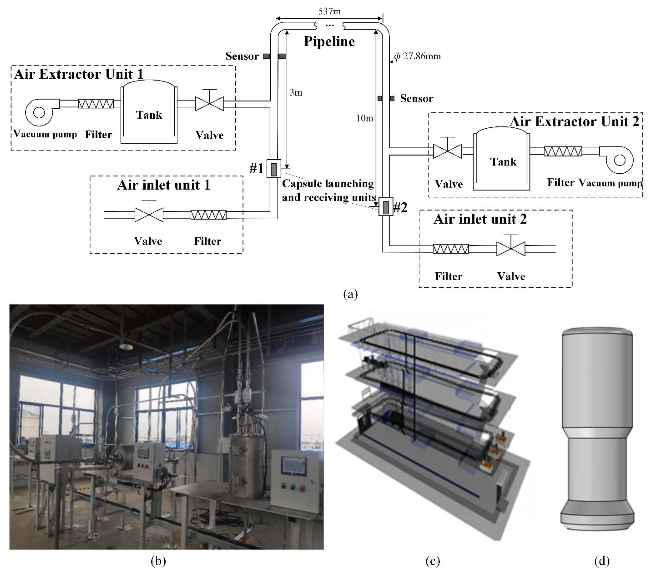
4.1.1. System Configuration

A testing PCP system was newly built in Jiangsu Shengtong Valve Co. Ltd., as shown in Figure 3. The system transports capsules between two capsule launching and receiving units (LRUs, as shown in Figure 3a) with vacuum pipelines. To transport a capsule from LRU-1 to LRU-2, the valve in the air extractor unit 2 (AEU-2) is switched on while all the other valves are switched off. The vacuum pump in AEU-2 is also turned on to extract the air out of the pipeline. Once a desired degree of vacuum has been produced, the valve in air inlet unit 1 (AIU-1) is switched on and the filtrated air rushes into the pipeline and drives the capsule to move forward to LRU-2. A series of velocity sensors were installed on the pipeline. When a capsule passes through a sensor, the transient speed of the capsule will be measured and recorded. Pressure sensors were also installed on the tanks to monitor the dynamic pressure variation during the process.

The 3D architecture of the PCP is shown in Figure 3b,c. The pipeline coils up on the three floors of a building and finally returns to the first floor. So, it composes of a series of straight/bent and vertical/horizontal segments. The total length of the pipeline is about 550 m, the inner diameter is D = 27.86 mm, and the turning radius of the bend segments is about 500 mm. The tested capsule (shown in Figure 3d), made of polyethylene, has an outer diameter of d = 22. The empty weight of the capsule is 20 g. In case a certain organic phase solution is loaded, the total weight can be up to 30 g.

4.1.2. Determination of the Coefficients

Different sections of pipelines with a unit length were modeled in 3D and then static CFD simulations were performed under various air flowrates conditions, as shown in Figure 4. The simulation was conducted on ANSYS Fluent 18.1 (Ansys Inc., Canonsburg, PA, USA) with the shear stress transport (SST) k−ω viscous model. At the inlets, the mass-flow-inlet boundary condition was used, while the pressure–outlet boundary condition was used at the outlets. Notably, the inlet flowrate is corresponding to the leakage flow rate (Q_l) rather than the total flow rate (Q) in case there is a capsule in the pipe section unit. Discretization of the governing equations was based on the QUICK or second-order upwind schemes. The velocity–pressure coupling was based on the SIMPLE algorithm, and the considered convergence criterion was 10⁻³.

Unstructured tetrahedral meshing was used to spatial discretize the flow domain. Refined mesh (mesh size s₁) was adopted in the vicinity of the capsule surfaces and coarser mesh (mesh size s₂) elsewhere. Gird independence tests were performed in advance by using gradually refined meshes with the same topology. Test case parameters were the inlet flow rate Q = 0.05 kg/s. The finally determined values are s₁ = 0.6 mm and s₂ = 2.0 mm, as shown in

Table 1. Grid independence test for the model of a capsule moving in a straight pipeline.

Mesh Size (mm)		No. of Elements	Pressure Drop (Pa)	Viscous FORCE (N)
s1	s2
2.9	0.9	166,097	1480.08	10.14
2.0	0.6	572,800	1823.02	12.50
1.5	0.3	1,539,626	1874.23	12.93

. The boundary layer mesh consisted of 10 layers with a 1.15 growth rate. The first layer thickness was adjusted depending on the boundary conditions to achieve a dimensionless wall distance y+ value below 5.

Once convergence was achieved, pressure drops in the pipe section units as well as viscous forces acting on the capsule surface corresponding to different inlet flowrates were extracted from the simulated results, and then the data were curve-fitted with quadratic polynomials. The simulated and curved fitted results regarding pressure drop are shown in Figure 5. The goodness of fit (R² > 0.9997) indicates the simple quadratic polynomials fit the simulated results very well. The obtained values of k₁ and k₂ are listed in

Table 2. Obtained values of k₁ and k₂ by 3D simulation and curve fitting.

Pipe Sections Types		k1 (×106 kg−1 m−2)	k2 (×103 m−2 s−1)
Straight	with a capsule	−13.19	−10.95
	without capsule	−0.78	−1.45
Bend	with a capsule	−24.06	−33.99
	without capsule	−0.84	−2.19

.

Data with regard to viscous forces were treated in a similar manner. The obtained values of k₃ and k₄ were 4.9 × 10³ (m/kg) and 5.1 (m/s), respectively. Due to the air-bearing effect as well as the light weight of the capsule, the friction force was found to be negligible, i.e., f = 0. The collision coefficients, k₅, were evaluated by experiments, in which the PCP was operated under a typical condition (initial pressure was 45 kPa) and the overall conveying time (OCT) was measured. The value of k₅ was adjusted from 0 to 1 until the best match of experimental and numerical OCT values was obtained. The finally determined value of k₅ is 0.35 (m⁻¹), which was used all through the following simulation.

4.1.3. Numerical Setting

Corresponding to 3D simulation, control volumes with a unit length were used to discrete the pipeline system in 1D simulation, i.e., the size of each control volume is Δx = 1 m. In order to obtain a compromise between computational effort and solution accuracy, a variable step size algorithm was applied, i.e.,

$$\mathsf{\Delta }t=\lambda \frac{\mathsf{\Delta }x}{v}$$

(20)

Different values of the coefficients λ had been tested and it was found independent results can be obtained when λ was below 0.005.

The boundary conditions were set corresponding to the actual operating conditions,

$$\begin{array}{l}\begin{array}{ccc}t=0& p=p_0& \end{array}\\ \begin{array}{ccc}t>0& \begin{array}{c}x=0\\ x=L\end{array}& \begin{array}{c}p=p_a\\ p=p_{\tan \mathrm{k}}^t\end{array}\end{array}\end{array}$$

(21)

where p₀ is the initial pressure in the pipeline system, and p_tank is the pressure of the tank shown in Figure 3a. According to the configuration of the system, the value of p_tank at an arbitrary time can be determined as

$$p_{\mathrm{tank}}^t={\rho }_{\mathrm{tank}}^{t}RT=p_0+RT{\displaystyle {\int }_0^t{Q}_L^{t}dt}/V_{\mathrm{tank}}$$

(22)

where Q_L^t is the transient outlet flow rate of the pipeline and V_tank is the volume of the tank.

4.2. Case 2

Data reported by Morikawa et al. [18] were also used for further model validation. The experimental setup consisted of a wheeled capsule which moved in a large-diameter pipeline (D = 125.6 mm, L = 30 m). Details of the system can be found in the literature [18,19].

Similar to other PCPs for heavy loads, the tested capsule had assembled with various sizes of plates on both ends (so-called end plates) to obtain larger drag force. In this case, viscous forces were found to be neglectable [8,11]. Furthermore, the pipeline is straight and horizontal, thus pressure force and friction force were the only forces contributing to capsule conveying. Pressure drop characteristics in the pipeline and pressure force acted on the capsule were estimated with the same method as illustrated in case 1. In the currently considered situation, the diameter ratio of end plates is 0.93, and the corresponding k₁ and k₂ values were determined as −3.61 × 10⁵ kg⁻¹ m⁻² and −3.04 × 10² m⁻² s⁻¹ for pipe section unit with a capsule, while they were −95 kg⁻¹ m⁻² and −11 m⁻² s⁻¹ for pipe section unit without capsule, respectively. The friction of wheels acting on the capsules had already been determined by experiments, and it can be given as [18]

$$F_f=0.235m+1.26$$

(23)

where the capsule weight m = 2.78 kg.

The numerical setting for the 1D simulation was all the same as that in case 1, except that a smaller size of CV, Δx = 0.05 m, was used. Boundary condition was set in accordance with the experimental procedure, i.e.,

$$\begin{array}{l}\begin{array}{ccc}t=0& p=p_0& \end{array}\\ \begin{array}{ccc}t>0& \{\begin{array}{c}x=0\begin{array}{cc}& p=\mathsf{\Phi }\left(Q\right)\end{array}\\ x=L\begin{array}{cc}& p=p_{a }\end{array}\end{array}& \begin{array}{c}\\ \end{array}\end{array}\end{array}$$

(24)

where Φ is a given function describing the characteristic diagram of the blowers used at the inlet [19].

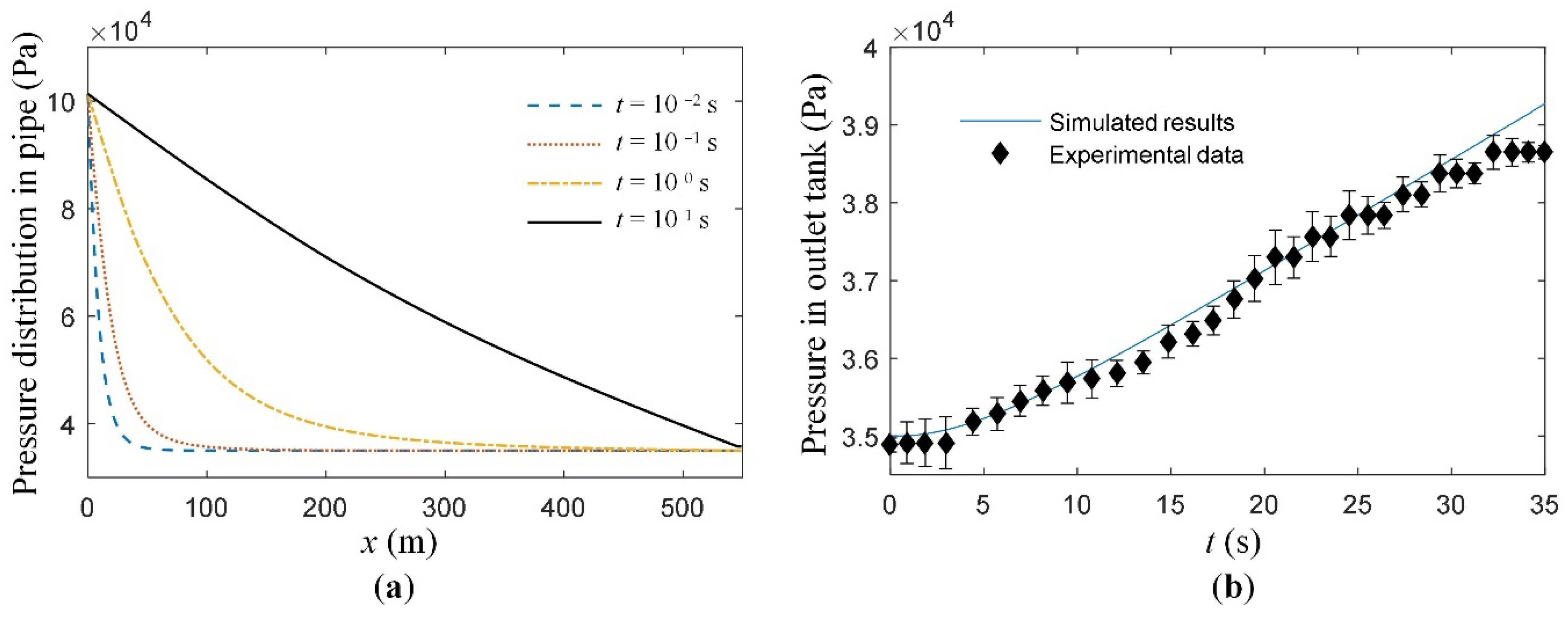
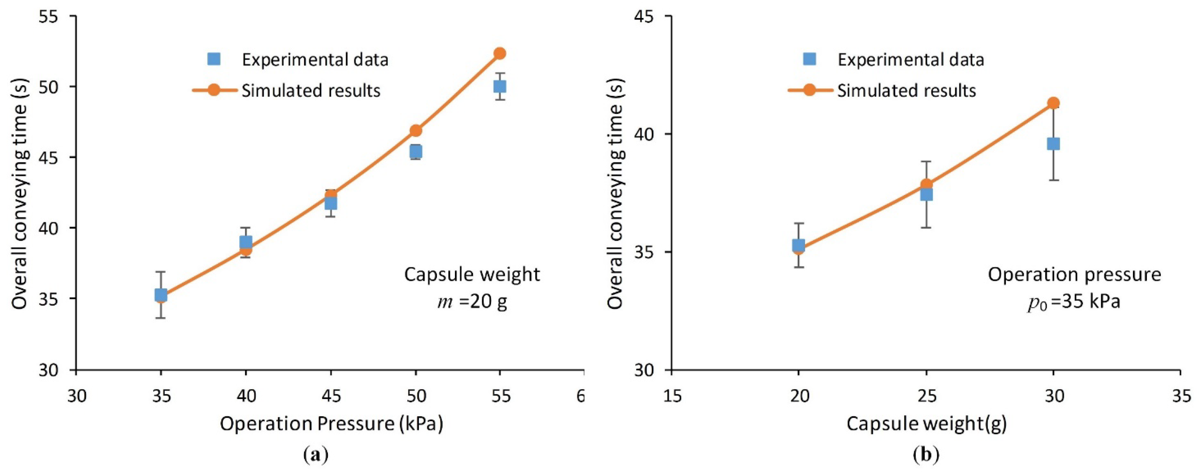
5. Results and Discussion

A series of experiments had been carried out using the testing PCP system shown in Figure 3 under various operation conditions. Each experiment was repeated for at least three times to obtain statistical results. Numerical simulations were performed correspondingly. A typical situation is illustrated herein, for instance, that is, the capsule is empty (m = 20 g), and the initial pressure of the system is p⁰ = 35 kPa (absolute pressure).

Capsule velocity results are presented in Figure 6. According to numerical simulation, the capsule is accelerated rapidly at the initial stage, and the transient speed increases by 40 m/s within a short distance (less than 3 m). Then the capsule is generally slowed down to a velocity of around 15 m/s. During the whole process, there are a series of velocity losses when the capsule is passing through the bend or vertical sections of the pipe, and also a series of subsequent procedures of velocity recovery in the following straight and horizontal sections. The simulated velocity profile was compared with the experimentally measured results to validate the model as well as the numerical method. As shown in Figure 6, the simulated and experimental results agree very well. The simulated OCT (35.12 s) is also very close to the experimental result (35.26 ± 0.92 s)

Further analysis with simulation demonstrates viscous force, rather than the pressure force, provides the main driven force at the initial stage due to the significant velocity difference between the airflow and the capsule, as shown in Figure 7. Such a result indicates that the aerodynamic configuration should be one of the main design considerations in developing a PCP system for the purpose of obtaining efficient capsule transportation. Along with the acceleration of the capsule, the viscous force decreases rapidly. As soon as the capsule moves faster than the airflow, viscous force becomes resistant.

The dynamic pressure distribution in the system was also predicted by simulation and presented in Figure 8. As soon as the process is initiated, the inlet pressure step into the atmosphere. Consequently, the pressure near the inlet increases rapidly while in the rest sections the pressure maintains at the initial level. As air flows forwards to the outlet, the overall pressure distribution evolves from a sharp profile at first to a linear profile generally, as shown in Figure 8a. The simulated dynamic pressure at the outlet (tank pressure) is compared with the experimentally measured results, which demonstrates high agreement again as shown in Figure 8b.

As one of the superiorities over those currently available models, the presented model has taken the compressibility of air into account, which would be significant in case the pipeline is very long [41]. However, the characteristic coefficients, k₁~k₅, were obtained by 3D CFD simulation with an incompressible flow model, which means the coefficients were assumed to be constants although they may vary to some extent under different pressure conditions. In addition, some factors, e.g., capsule weight, have a certain impact on the posture of the capsule in the pipeline. Consequently, the flow profile and conveying process may be impacted. However, an ideal capsule posture was assumed in the 3D simulation. These simplifications may be the most important limitations of the presented method. To evaluate the impact of such simplifications on the accuracy of model prediction, a series of contrast simulations were performed with different pressure levels (from normal pressure to −50 kPa) and capsule postures (concentric and eccentric positions). It was demonstrated the variation of resulted model coefficients was within 10%. Furthermore, experiments had also been conducted under different operation conditions. Simulation with constant coefficient values (given in Section 4.1.2) was performed accordingly and the OCT values were used for comparison. As shown in Figure 9, the simulated values agree with the experimental results very well. The maximum error was only 4.43% among all the considered conditions, demonstrating that errors induced by the simplifications are acceptable in practice. By accurately predicting systemic behavior of PCPs in a relatively simple manner, the presented method can be used to evaluate the effect of every design parameter on system performance in detail, and then the optimal design may be achieved.

In addition to the light-load PCPs (like the testing system in case 1), there are also PCPs used for conveying minerals, freight, and other heavy loads in the industry. The pipelines have large diameters, and the capsules have much larger sizes and are usually constructed with wheels and end plates. In order to examine the applicability of the presented method for predicting such PCP systems, a set of experimental data reported in the literature were also used for validation.

As shown in Figure 10, the simulated profiles of velocity and pressure agree well with the experimental data. The predicted OCT (2.68 s) and maximum capsule velocity (9.65 m/s) are very close to the report values (2.7 s and 9.72 m/s), with a relative error of only 0.74% and 0.72%, respectively. Such extremely high accuracy was obtained partly because of the simple (straight only) and short (30 m) pipeline used in the experiments. Another analytical model also gave a comparable prediction in this case [19]. But for the practical systems used in industry, the analytical model, which overlooked the complexity of pipe configuration and air compressibility, will be not applicable anymore.

6. Conclusions

In this work, a novel method is presented to evaluate the performance of PCPs. A one-dimensional model is established to describe the systemic behavior of PCPs, i.e., the dynamic processes of airflow and capsule motion. The model is simple but still accounts for those phenomena that most profoundly affect the performance of PCPs, such as: the 3D architecture of pipelines, the geometry of capsules, the compressibility of air in long-distance pipelines, as well as the operating conditions of the PCP systems, and so on. Three-dimensional simulation is used to model the local process and obtain the characteristic coefficients in the 1D model. A numerical method is also presented to solve the model equations. With a given pipeline configuration, capsule properties, and operating conditions, the capsule conveying and other related processes can be predicted.

The method has been validated by comparing model predictions with experimental data with respect to two different types of PCPs. The first one has a small diameter (27.86 mm), long-distance (550 m), and 3D-layout pipeline, and the capsule has a relatively complex aerodynamic geometry. Even so, the model prediction achieved favorable accuracy (errors within 4.43%). To our knowledge, it is the first time to report successful simulation of such a complicated but practical PCP system. The second one has a large-diameter (125.6 mm) and a relatively short (30 m) pipeline, and the capsule has been assembled with wheels and end plates. Excellent accuracy was obtained again (errors within 1%), demonstrating the high applicability of the presented method for various PCPs. By rapidly and accurately predicting the overall performance, the presented method provides an effective tool for screening the optimal parameters in the design and application of PCP systems.

References

1. Kosugi, S. A Capsule Pipeline System for Limestone Transport. In Proceedings of the 4th International Conference on Bulk Materials, Storage, Handling and Transportation: 7th International Symposium on Freight Pipelines, Wollongong, Australia, 6–8 July 1992; Volume 7, pp. 13–17. [Google Scholar] [CrossRef]
2. Hane, K.; Okutsu, K.; Matsui, N.; Kosugi, S. Applicability of pneumatic capsule pipeline system to radioactive waste diposal facility. In Proceedings of the WM’02 Conference, Tucson, AZ, USA, 24–28 February 2002. [Google Scholar]
3. Hidalgo, D.; Martín-Marroquín, J.M.; Corona, F.; Juaristi, J.L. Sustainable vacuum waste collection systems in areas of difficult access. Tunn. Undergr. Space Technol. 2018, 81, 221–227. [Google Scholar] [CrossRef]
4. Farré, J.A.; Salgado-Pizarro, R.; Martín, M.; Zsembinszki, G.; Gasia, J.; Cabeza, L.F.; Barreneche, C.; Fernández, A.I. Case study of pipeline failure analysis from two automated vacuum collection system. Waste Manag. 2021, 126, 643–651. [Google Scholar] [CrossRef] [PubMed]
5. Liu, H. Pneumatic capsule pipeline-basic concept, practical considerations, and current research. Mid-Cont. Transp. Symp. 2000, 230, 230–234. [Google Scholar]
6. Shibani, W.M.; Zulkafli, M.F.; Basuno, B. Methods of transport technologies: A review on using tube/tunnel systems. IOP Conf. Ser. Mater. Sci. Eng. 2016, 160, 012042. [Google Scholar] [CrossRef]
7. Okutsu, K.; Esaki, T.; Matsui, N.; Fukunaga, T.; Saito, K. Comprehensive pneumatic transportation system for geological disposal facilities. In Proceedings of the WM’04 Conference, Tucson, AZ, USA, 29 February–4 March 2004. [Google Scholar]
8. Turkowski, M.; Szudarek, M. Pipeline system for transporting consumer goods, parcels and mail in capsules. Tunn. Undergr. Space Technol. 2019, 93, 103057. [Google Scholar] [CrossRef]
9. Kosugi, S. Pneumatic capsule pipelines in Japan and future developments. Handb. Powder Technol. 2001, 10, 501–511. [Google Scholar] [CrossRef]
10. Belova, O.V.; Vulf, M.D. Pneumatic capsule transport. Procedia Eng. 2016, 152, 276–280. [Google Scholar] [CrossRef] [Green Version]
11. York, K.; Liu, H. Predicting drag coefficient of pneumatic capsule. J. Transp. Eng. 2001, 127, 390–397. [Google Scholar] [CrossRef]
12. Kosugi, S. Effect of traveling resistance factor on pneumatic capsule pipeline system. Powder Technol. 1999, 104, 227–232. [Google Scholar] [CrossRef]
13. Ohashi, A.; Yanaida, K. The fluid mechanics of capsule pipelines: 1st report, analysis of the required pressure drop for hydraulic and pneumatic capsules. Bull. JSME 1986, 29, 1719–1725. [Google Scholar] [CrossRef]
14. Ohashi, A.; Yanaida, K. The fluid mechanics of capsule pipelines: 2nd report, analysis of the pressure loss in concentric capsules, pipelines and annular pipes. Bull. JSME 1986, 29, 4156–4163. [Google Scholar] [CrossRef] [Green Version]
15. Ohashi, A.; Yanaida, K. The fluid mechanics of capsule pipelines: 3rd report, analysis of the pressure loss in eccentric capsules pipelines and eccentric annular pipes. Bull. JSME 1986, 29, 3779–3786. [Google Scholar] [CrossRef]
16. Liu, H.; Kosugi, S. Use of Pneumatic Capsule Pipeline for Underground Tunneling. In Proceedings of the 12th International Symposium on Freight Pipelines, Prague, Czech Republic, 20–24 September 2004. [Google Scholar]
17. Liu, H. Feasibility of Using Pneumatic Capsule Pipelines in New York City for Underground Freight Transport. In Proceedings of the ASCE Pipeline Division Specialty Congress, San Diego, CA, USA, 1–4 August 2004; pp. 1–12. [Google Scholar]
18. Morikawa, Y.; Tsuji, Y.; Chono, S.; Yoshida, H. A Fundamental Investigation of the Capsule Transport: 3rd Report, Friction of Capsule Wheels and Transport Experiment of a Single Capsule. Bull. JSME 1984, 27, 2181–2187. [Google Scholar] [CrossRef] [Green Version]
19. Tsuji, Y.; Morikawa, Y.; Chono, S.; Imae, H.; Yoshikawa, T. A Fundamental Investigation of the Capsule Transport: 4th Report, Numerical Analysis of Motion of Accelerating and Decelerating Capsules. Bull. JSME 1985, 28, 1128–1134. [Google Scholar] [CrossRef] [Green Version]
20. Tomita, Y. Numerical analysis of pneumatic capsule pipeline system: Continuous loading with short intervals. Bull. JSME 1985, 28, 2480–2481. [Google Scholar] [CrossRef]
21. Wee Chuan Lim, E.; Wang, C.-H.; Yu, A.-B. Discrete element simulation for pneumatic conveying of granular material. AIChE J. 2006, 52, 496–509. [Google Scholar] [CrossRef]
22. Wang, Y.; Williams, K.; Jones, M.; Chen, B. CFD simulation methodology for gas-solid flow in bypass pneumatic conveying—A review. Appl. Therm. Eng. 2017, 125, 185–208. [Google Scholar] [CrossRef]
23. Miao, Z.; Kuang, S.; Zughbi, H.; Yu, A. CFD simulation of dilute-phase pneumatic conveying of powders. Powder Technol. 2019, 349, 70–83. [Google Scholar] [CrossRef]
24. Nguyen, D.; Rasmuson, A.; Niklasson Björn, I.; Thalberg, K. CFD simulation of transient particle mixing in a high shear mixer. Powder Technol. 2014, 258, 324–330. [Google Scholar] [CrossRef]
25. Kuang, S.; Zhou, M.; Yu, A. CFD-DEM modelling and simulation of pneumatic conveying: A review. Powder Technol. 2020, 365, 186–207. [Google Scholar] [CrossRef]
26. Shi, Q.; Sakai, M. Recent progress on the discrete element method simulations for powder transport systems: A review. Adv. Powder Technol. 2022, 33, 103664. [Google Scholar] [CrossRef]
27. Towler, G.; Sinnott, R. Chapter 18-Specification and design of solids-handling equipment. In Chemical Engineering Design, 3rd ed.; Towler, G., Sinnott, R., Eds.; Butterworth-Heinemann: Oxford, UK, 2022; pp. 735–821. [Google Scholar]
28. Huber, N.; Sommerfeld, M. Modelling and numerical calculation of dilute-phase pneumatic conveying in pipe systems. Powder Technol. 1998, 99, 90–101. [Google Scholar] [CrossRef]
29. Tashiro, H.; Peng, X.; Tomita, Y. Numerical prediction of saltation velocity for gas-solid two-phase flow in a horizontal pipe. Powder Technol. 1997, 91, 141–146. [Google Scholar] [CrossRef]
30. Levy, A. Two-fluid approach for plug flow simulations in horizontal pneumatic conveying. Powder Technol. 2000, 112, 263–272. [Google Scholar] [CrossRef]
31. Tsuji, Y.; Tanaka, T.; Ishida, T. Lagrangian numerical simulation of plug flow of cohesionless particles in a horizontal pipe. Powder Technol. 1992, 71, 239–250. [Google Scholar] [CrossRef]
32. Le, T.T.G.; Jang, K.S.; Lee, K.-S.; Ryu, J. Numerical Investigation of Aerodynamic Drag and Pressure Waves in Hyperloop Systems. Mathematics 2020, 8, 1973. [Google Scholar] [CrossRef]
33. Al-Obaidi, A.R. Numerical investigation on effect of various pump rotational speeds on performance of centrifugal pump based on CFD analysis technique. Int. J. Model. Simul. Sci. Comput. 2021, 12, 2150045. [Google Scholar] [CrossRef]
34. Al-Obaidi, A.R.; Qubian, A. Effect of outlet impeller diameter on performance prediction of centrifugal pump under single-phase and cavitation flow conditions. Int. J. Nonlinear Sci. Numer. Simul. 2022. [Google Scholar] [CrossRef]
35. Feng, J.; Huang, P.Y.; Joseph, D.D. Dynamic simulation of the motion of capsules in pipelines. J. Fluid Mech. 1995, 286, 201–227. [Google Scholar] [CrossRef]
36. Asim, T.; Mishra, R. Computational fluid dynamics based optimal design of hydraulic capsule pipelines transporting cylindrical capsules. Powder Technol. 2016, 295, 180–201. [Google Scholar] [CrossRef]
37. Dupont, C.; Le Tallec, P.; Barthès-Biesel, D.; Vidrascu, M.; Salsac, A.-V. Dynamics of a spherical capsule in a planar hyperbolic flow: Influence of bending resistance. Procedia IUTAM 2015, 16, 70–79. [Google Scholar] [CrossRef]
38. Zhang, C.; Sun, X.; Li, Y.; Zhang, X.; Zhang, X.; Yang, X.; Li, F. Hydraulic characteristics of transporting a piped carriage in a horizontal pipe based on the bidirectional fluid-structure interaction. Math. Probl. Eng. 2018, 2018, 8317843. [Google Scholar] [CrossRef]
39. Abushaala, S.; Shaneb, A.; Enbais, F.; Abulifa, A. Hydrodynamic analysis of pipelines transporting capsule for onshore applications. Int. J. Eng. Inf. Technol. 2018, 5, 53–62. [Google Scholar]
40. Khani, D.; Lim, Y.H.; Malekpour, A. Calculating Column Separation in Liquid Pipelines Using a 1D-CFD Coupled Model. Mathematics 2022, 10, 1960. [Google Scholar] [CrossRef]
41. Herrán-González, A.; De La Cruz, J.M.; De Andrés-Toro, B.; Risco-Martín, J.L. Modeling and simulation of a gas distribution pipeline network. Appl. Math. Model. 2009, 33, 1584–1600. [Google Scholar] [CrossRef]
42. Yuan, Z.; Deng, Z.; Jiang, M.; Xie, Y.; Wu, Y. A modeling and analytical solution for transient flow in natural gas pipelines with extended partial blockage. J. Nat. Gas Sci. Eng. 2015, 22, 141–149. [Google Scholar] [CrossRef]
43. Patankar, S.V. Numerical Heat Transfer and Fluid Flow; Hemisphere Publishing Corporation: London, UK, 1980. [Google Scholar]
Figure 1. Schematic diagram of force analysis for capsules moving in PCP.
Mathematics 10 04073 g001
Figure 2. Illustration of the discrete control volumes.
Mathematics 10 04073 g002
Figure 3. The testing PCP system (a) Schematic of the PCP system (b) Real view of the PCP system (c) 3D architecture of the pipeline (d) Configuration of the capsule.
Mathematics 10 04073 g003
Figure 4. Illustration of the models in 3D CFD simulation.
Mathematics 10 04073 g004
Figure 5. Simulated pressure drop characteristics of various pipe-section units: (a) straight-without capsule; (b) straight-with a capsule; (c) bend-without capsule; (d) bend-with a capsule.
Mathematics 10 04073 g005
Figure 6. Simulated and experimentally measured velocity profiles of the capsule.
Mathematics 10 04073 g006
Figure 7. Calculated forces acted on the capsule at the initial stage.
Mathematics 10 04073 g007
Figure 8. Dynamic of pressure in the pipeline (a) and in outlet tank (b).
Mathematics 10 04073 g008
Figure 9. Experimental and simulated overall conveying time with various operation pressure (a) and capsule weight (b).
Mathematics 10 04073 g009
Figure 10. Comparison of simulated results with literature data: (a) capsule velocity and air velocity behind the start point of the capsule; (b) air pressure at the flow inlet.
Mathematics 10 04073 g010