Deep Reinforcement Learning for Crowdshipping Last-Mile Delivery with Endogenous Uncertainty

Abstract

In this work, we study a flexible compensation scheme for last-mile delivery where a company outsources part of the activity of delivering products to its customers to occasional drivers (ODs), under a scheme named crowdshipping. All deliveries are completed at the minimum total cost incurred with their vehicles and drivers plus the compensation paid to the ODs. The company decides on the best compensation scheme to offer to the ODs at the planning stage. We model our problem based on a stochastic and dynamic environment where delivery orders and ODs volunteering to make deliveries present themselves randomly within fixed time windows. The uncertainty is endogenous in the sense that the compensation paid to ODs influences their availability. We develop a deep reinforcement learning (DRL) algorithm that can deal with large instances while focusing on the quality of the solution: we combine the combinatorial structure of the action space with the neural network of the approximated value function, involving techniques from machine learning and integer optimization. The results show the effectiveness of the DRL approach by examining out-of-sample performance and that it is suitable to process large samples of uncertain data, which induces better solutions.

1. Introduction

Last-mile delivery is a term used to define the transportation of items from a depot to a final customer destination. Last-mile delivery is evolving at a rapid rate and has become a topic of great interest due to the increase in e-commerce in recent years, making it a key differentiator among large competitors in this sector.

We study a business model where the company outsources part of the activity of delivering products to its customers to occasional drivers, also known as crowdshipping, complementing its own fleet. All deliveries are completed at the minimum total cost incurred with the company vehicles and drivers plus the compensation paid to the ODs. The company decides on the best compensation scheme to offer to the ODs at the planning stage.

Crowd-shipped delivery has been adopted as a shortcut to last-mile growth. It has been implemented under different business models depending on how the occasional drivers are engaged and managed. A survey in [1] indicates that while only 9% of retailers are using crowd-sourced providers now, one in four retailers plans to start using them in the next 12 months. It has been implemented as an enabler to same-day delivery for the last mile as can be seen in recent implementations of large companies as in [2,3,4].

This setting also potentiates greater efficiency by making better use of existing urban traffic flows. For example, the case of crowdshipping with in-store customers taking up delivery tasks on their way home to serve online customers. As a result of fewer freight vehicles being used, the company’s costs are reduced while also benefiting society from the reduced traffic congestion.

Our setup is suitable for a same-day delivery scheme where time windows are fixed, predefined periods during the day and customers with online orders and available occasional drivers can enlist themselves in these time windows.

Crowdshipping last-mile delivery has been modeled as a variation of the vehicle routing problem (VRP) or the traveling salesman problem (TSP), under different deterministic, stochastic, and/or dynamic optimization approaches (e.g., [5,6,7,8,9]).

A general topic presented in these works relates to the compensation offered to occasional drivers. Choosing an appropriate compensation scheme is challenging. Different compensation schemes presented in the literature have both advantages and disadvantages associated with them. It can affect the number of available occasional drivers and also which customer locations will be assigned to occasional drivers and not to the company’s drivers, affecting overall cost savings.

In general, all the compensation schemes proposed in the literature so far are static schemes (see Section 2), in the sense that the decision-maker cannot decide on different compensation rates levels paid to the occasional drivers.

In this work, a flexible compensation scheme is proposed taking into account the occasional driver’s willingness to engage in a delivery task. Flexible pricing systems are still a recent subject under study in the crowdshipping literature and with only a few implementations (e.g., [10]).

We are interested in analyzing the effect of the compensation level decision not only on the solution provided to our problem but also on the complexity associated with its resolution.

We adopt a data-driven dynamic and stochastic approach where the existence of online customers’ orders to be delivered, as well as the availability of occasional drivers to deliver them, are random and define scenarios on which decisions have to be made.

This problem is complex because decisions, regarding the dispatch of vehicles or occasional drivers, have to be made fast and the space to search for decisions is potentially too large. Here, we extend the work initiated in [11] and propose a deep reinforcement learning (DRL) method where we model the problem as a sequence of states connected by actions, driven by decisions, and transitions. The DRL method uses a neural network (NN) as an approximation architecture for the problem value function. Our approach is data-driven: we make use of a generative method, exploiting available scenario historical data, to generate additional scenarios, that in turn are used to train the DRL neural network.

Another key feature of our DRL approach is how we search the action (decision) space. Most reinforcement learning (RL) studies on stochastic VRPs face the challenge imposed by the combinatorial nature of state and action spaces by restricting the action space and aggregating the state space based on expert knowledge. Here, we formulate the action selection problem for each state using a recourse in a two-stage decision model where the first-stage decision is formulated as a mixed-integer optimization program. In the first stage, not only the order in which all customers will be delivered is established, as in [11], but also the best compensation to be paid for the outsourcing of each customer. The second-stage decision is made every time a scenario is revealed, and before any dispatch of fleet vehicles or ODs. The second-stage decision comprises routes defined by the recourse, where the routes follow the first-stage decision ordering but skip customers that have no online orders or customers outsourced for available ODs. Each time the vehicle capacity or the time window limit is reached, a return path to the depot is created and another route restarts from the depot if needed.

The main contributions of the approach above and the results of this work are:

• We propose a novel data-driven stochastic and dynamic approach for crowdshipping last-mile delivery, where we introduce a flexible compensation scheme, advancing the state-of-the-art in this topic.
• We experiment with generative methods to create new scenarios to train our neural network. Historical data are typically in small amounts and inadequate to evaluate the policies of our DRL approach. We exploit the fact that there is time correlation information hidden between scenarios included in the historical data. We learn this time correlation using conditional generative adversarial networks and use them as a tool to generate scenarios to evaluate our policies.
• We present computational results on the capability of the proposed model, assuming a realistic point-of-view of correlated scenarios.

In the sequence of this work, in Section 2, we present relevant approaches to solve problem variants. In Section 3, we present our problem description and the defined model. In Section 4 we introduce the DRL method developed. Next, in Section 5, we discuss the computational results. Finally, in Section 6, we present this work’s conclusions.

2. Literature Review

In the following sections, we survey relevant literature for the proposed approach. It includes not only the publications related to models for the crowdshipping of last-mile delivery, in particular in the different approaches developed to deal with the compensation of occasional drivers, but also covers the approaches for the problems where the customers are uncertain and applications of RL methods to VRPs.

2.1. Crowdshipping Routing and Compensation Schemes

In [5], the authors developed the first work on crowdshipping last-mile delivery. The authors study a deterministic approach where data such as the customers’ locations, parameters used to define occasional drivers’ compensation fees, and which customers an occasional driver can outsource, are used as input. The model proposed is a combination of an assignment problem for occasional drivers, with a capacitated VRP where vehicle routes are defined for customers not assigned to occasional drivers. A customer is assigned to an occasional driver only if it is overall optimal. The compensation scheme is then an important part of the proposed algorithm. In a basic variant of their problem, the compensation fee paid to an occasional driver is proportional to the distance between the depot and the customer location and does not consider the destination of the occasional driver. They argue the practical advantages of this method since the company only deals with the location of its customers, but it is non-ideal for occasional drivers because it does not consider the extra costs incurred. A variant is proposed where the occasional driver is paid proportionally to the detour from their original route between the depot and their final destination. The authors argue that this is more challenging to implement because it demands registering the occasional driver’s destination. They suggest that new and innovative compensation schemes are essential to further developments on this subject.

Using the models above, the authors can exercise the potential benefits of employing occasional drivers to make deliveries. They analyze results based on: (1) the number of occasional drivers available regarding the number of customers; (2) how much flexibility exists in terms of an allowed detour from an occasional driver’s original route and; (3) what compensation scheme is used and the amount an occasional driver is paid. They conclude that designing an adequate compensation scheme is one of the most important challenges for a company to define.

The authors in [8] study a dynamic and stochastic approach in which the demand, as online orders, arrives over time, as do in-store customers available to make deliveries. They present rolling horizon dispatching algorithms: one that exploits only the present state of the systems, and one that also exploits probabilistic data concerning future delivery orders and customers available to make deliveries arrivals. The compensation includes two terms. One term reflects a fixed compensation paid to in-store customers who deliver orders. The second term is proportional to the online order delivery time. Through numerical experiments, they verify that the quality of service may increase and the operational costs may decrease if the delivery capacity is augmented by the application of higher compensation fees to in-store customers. They study the sensitivity of these customers to price. Higher compensation can incur more participation but also become a less attractive alternative. As a consequence, crowdshipping may become simply the backup plan.

In [12], the authors assume occasional drivers that arrive randomly. Routes are developed for professional vehicles and the occasional drivers considering their final destination. Occasional drivers appear in defined time windows. They develop a two-stage model in which professional vehicle routes are defined in the first stage and, as occasional drivers appear, they adjust deliveries in the second stage. There is a paid penalty for customers that are not served. We note that here the uncertain event is related to the presence of a given occasional driver. Their stochastic solution is based on a scenario approach with a uniform distribution. They conduct computational experiments where they limit the size of the instances to 20 customers and 3 occasional drivers. Three alternative compensation schemes are analyzed: (1) a fixed and equal compensation fee is paid for each served request; (2) the compensation fee is proportional to the traveling distance from a pickup to the delivery location; and (3) the compensation fee is proportional to the detour distance made by the occasional driver. The computational results show that using occasional drivers can produce savings even when a suboptimal compensation scheme is used.

In an attempt to capture some randomness in the process of acceptance by occasional drivers, the authors in [6] investigate a stochastic approach to the problem. There, customers are either offered or not to potential occasional drivers and the acceptance probability is known. A heuristic is used to identify customers’ orders to be offered to occasional drivers. They emphasize the relationship between the compensation offered to occasional drivers, the probability of their acceptance, and the resolution of the customer set offered to outsource. We note that here that the uncertain event is related to the customer being outsourced.

In [9], the authors assume a dynamic environment, where the solution is adjusted each time information becomes available. A service platform matches parcel delivery tasks to ad hoc drivers. An exact solution approach using a rolling horizon framework is developed. Compensations are defined as being proportional to the cost of serving all customers without occasional drivers. The authors present examples of crowdsourcing delivery platforms that offer same-day delivery and compare their respective compensation schemes that vary between hourly rates and per-package remuneration.

The section’s references above provide interesting results regarding the importance of the definition of the correct compensation scheme, but they all offer post-optimal sensitivity analysis. This limitation has inspired this work to study alternatives for more flexible compensation schemes where the compensation paid to ODs can be part of the decision made by decision-makers.

A survey by [13] analyzes the status of crowdshipping and provides a classification of available platforms. The authors also review the operations research literature explicitly addressing this topic.

2.2. Routing with Customer Uncertainty

Stochastic optimization approaches to routing problems based on customer uncertainty have been studied by many authors.

A seminal work addressing routing with customer uncertainty was studied in [14]. The authors define a routing problem where only a random subset of customers are served. The problem is defined as the Probabilistic Traveling Salesman Problem. They develop closed-form expressions for the expected length of any route, given that customers’ probability distributions are independent.

The study above is extended in [15], where the authors define a stochastic variant of the VRP. There, customer demands and/or customer presence are stochastic. The authors define a recourse strategy where absent or no-demand customers are skipped in pre-defined routes. Additionally, routes are split and a detour back to the depot occurs when the vehicle capacity is reached. The authors elaborate on the need to define strategic planning solutions, where an a priori service customer sequence of minimal expected length is calculated, rather than solving the problem only when the demand or presence is known. They develop closed-form expressions and algorithms to compute the expected length of an a priori sequence, given that customers’ probability distributions are independent.

Branch-and-cut integer L-Shaped algorithms were developed in [16] and in [17] to solve the two models above. The authors could solve instances with up to nine uncertain customers. In [18], improvements were introduced to the branch-and-cut integer L-Shaped algorithm developing, among others, stronger lower-bounds formulations. Instances with 25 to 100 vertices and 2 to 4 vehicles were optimally solved for Poisson and normal demand distributions.

In [19], assuming stochastic demands, the authors developed a branch-cut-and-price algorithm for the VRP. They formulated it as a set partitioning model with additional constraints and improved the algorithm performance significantly. They developed the ng-routes that are used for the pricing sub-problems together with routines for 2-cycle elimination.

A branch-and-bound algorithm is developed in [20] for the probabilistic TSP, using the same concept of a priori strategy defined in [15]. They extend previous deterministic TSP algorithms, leveraging the closed expected value evaluation expression of [14]. The authors additionally present in [21] another branch-and-bound algorithm exploiting parallelization techniques and solving instances for up to 30 customers.

An approximation scheme is developed in [22] for the VRP with stochastic customers. A two-stage stochastic optimization set-partitioning formulation is presented where a set of vehicle routes serving all customer locations is defined a priori before any service request is known. The uncertain events are assumed to be independent. A column generation framework that allows for solving the problem to a given optimality tolerance is proposed. They solve instances for up to 40 customers within the time limit of six hours.

A heuristic approach for solving the VRP with stochastic demand, using a set-partitioning formulation, is presented in [23]. First, it presents a heuristic to define a good finite set of feasible routes that are used as columns to solve the problem. Furthermore, a recourse approach is developed, where vehicles can serve additional customers from failed routes before going back to the depot or they can serve customers from failed routes on a new route after going back to the depot. Instances of 75 customers are solved.

The stochastic studies in this section assume that the uncertain events are independent. In many real-life problems, although, event correlation can contain important information to be considered in the solution. These correlations are often difficult to deal with, which makes the planning problem complicated. An alternative is a modeling approach that considers the worst-case joint distribution, under the theory of Distributionally Robust Optimization (DRO—see, [24,25,26]). After identifying a set $\mathcal{P}$ of allowable probability distributions that include the true distribution $\mathbb{P}$, and called the ambiguity set, the objective function is reformulated concerning the worst-case expected cost over all possible distributions in the ambiguity set.

The authors in [27] present a VRP with stochastic demands with no recourse where an important feature of the methodologies presented allows random events correlation. Another characteristic is that chance constraints are used to limit the infeasibility of the routes due to capacity limits. The authors propose the use of a branch-price-and-cut algorithm. They identify that the pricing subproblem is strongly NP-hard, even if the priced routes have cycles. They identify further route relaxation alternatives and develop pricing algorithms through the use of dynamic programming. They solve instances for up to 55 customers.

In [28], the authors study a variant of the capacitated VRP with no recourse where an ambiguity set is known for the demand random vector. They also present a chance-constrained formulation and show that it can be solved with standard branch-and-cut algorithms when the ambiguity set satisfies a certain subadditivity condition.

2.3. Reinforcement Learning for Routing

Most works with an RL approach to solving the VRP interpret it as a Markov Decision Process, in which the optimal solution is viewed as a sequence of actions deciding which customer to visit according to the state revealed. They draw on the concept of policy-gradient or value-function approximation (VFA). Policy-gradient methods search directly for an optimal policy and do not have to be concerned with the value function. In general, the policy is parametrized. VFAs approximate the value of post-decision states using simulations. The values are stored usually in functions or tables. The challenge is related to the fact that the VRP, as combinatorial optimization problems in general, can have large combinatorial action spaces. The VRP high-dimensional action space turns methods that approximate state-action pair values inviable because they enumerate all possible actions. Typically, as an alternative, the action space is restricted instead.

The authors in [29] present one of the first studies involving RL methods to solve routing problems. They train a recurrent neural network for the TSP, called a pointer network. Given a set of city coordinates, it predicts a distribution over different city permutations. They developed a policy gradient algorithm to optimize the parameters of the recurrent neural network.

Motivated by the work in [29], the authors in [30] generalize to include other combinatorial optimization problems such as the VRP. They propose an alternate approach in which the policy model consists of a recurrent neural network decoder together with an attention mechanism and apply a policy-gradient approach.

An alternative to the approach of reducing the action space with VFA is presented in the work of [31]. They present a value-function-based DRL algorithm. The action selection problem is formulated as a mixed-integer optimization problem and is able to exploit the whole combinatorial action space. They focus on the Capacitated Vehicle Routing Problem. There, a capacity-constrained vehicle must be assigned one or more routes to serve customers with demands and minimize traveled distance. ReLU activations are used, exploiting the work developed in [32] for strong MILP reformulations of neural network-related problems.

With business models shifting to same-day delivery, routing problems have become increasingly stochastic and dynamic. A problem class called the stochastic dynamic vehicle routing problem (SDVRP) arises and poses new challenges as they require anticipatory real-time routing actions and static solutions are no longer adequate. Recent works have shown that RL appears to be a good solution method for dynamic combinatorial optimization as the SDVRP.

In [33], the authors present an actor-critic framework and apply a policy-based RL algorithm for the problem of pick-ups at customers with dynamic service requests. They consider dynamic requests and customer locations that are unknown in advance. They extend a policy learned for a single vehicle to all vehicles.

In [34], the authors present the first study to implement deep Q-learning methods for same-day delivery problems with a heterogeneous fleet of vehicles and drones. Their method learns the value of assigning a new customer to either drones or vehicles as well as the option to not offer service at all. They reduce the state space to a set of selected features and define it in a way to make it possible to enumerate alternative actions at the decision points.

A survey by [35] highlights the potential of RL methods applied to VRPs from the point of view of operations research and computer science communities and guide to joint approaches to overcome current obstacles. Overall, they suggest: (1) methods combining piece-wise linear neural network VFAs and solvers searching the action space; (2) policy-based methods that overcome the combinatorial action space; and (3) multi-agent RL approaches together with searching the joint action space with a global MIP.

2.4. Stochastic Optimization with Endogenous Uncertainty

The works presented in Section 2.2 are based on the assumption that the stochastic process is independent of the optimization decisions. Here, we consider the case of decision-making for an application that is not only subject to uncertainty but where decisions affect future uncertainties as well. In these cases, the uncertainty is endogenous or ‘decision-dependent’.

Even though such uncertainties prevail in real-life settings, these problems have not received the deserved attention in the past, mainly because of computational burdens. Nevertheless, considering this dependency can be an important step in improving system performance. Since the work in [36], dealing with a Markovian process, which first addresses the case with endogenous uncertainty, other approaches to this type of problem have been studied.

The authors in [37] first addressed problems with endogenous uncertainty where project decisions, instead of affecting the probability distribution themselves, give more information that is used to resolve the uncertainty instead. They assume that the cost of an item is uncertain until the moment it is produced. The probability distribution depends on which item is produced and when.

In [38], the authors address the offshore oil and gas planning problem to maximize revenues and investments over some time. The oil fields’ size is not known in advance. The authors present a disjunctive formulation with non-anticipativity constraints to capture the interaction between the decisions and the resolution of uncertainty.

In [39], the authors extend the previous approach to a multistage stochastic problem for optimal production scheduling, that minimizes cost while satisfying the demand for different goods. Here, they consider endogenous uncertainty where the project decisions lead to the resolution of uncertainty.

Endogenous uncertainty has also been studied under distributionally robust optimization assumptions. Here, the set $\mathcal{P}$ of feasible probability distributions can depend on the first-stage decision variables. This leads to solving a Decision-Dependent Distributionally Robust Problem.

The authors in [40] developed a framework that includes two-stage decision-dependent distributionally robust stochastic programming as a special case and considers five types of ambiguity sets for which they offer reformulations designed for specific resolutions.

Another interesting application of endogenous uncertainty is within dynamic pricing, being a field of revenue management. Here, a company adjusts prices according to inventories left and the demand response observed. The decision to set prices at different levels influences the future demand for the products being priced. Among others, this application has been addressed under different approaches of reinforcement learning techniques (e.g., [41,42] ). In fact, reinforcement learning has grown to represent a broad problem class of sequential stochastic optimal decision problems.

3. Stochastic Crowd Shipping Last-Mile Delivery with Endogenous Uncertainty

We follow [11] and define a typical setting for our problem in which a store is the location for in-store customers and also the depot from where online customer orders are dispatched. In-store customers who are available to deliver online customers’ orders on their way back home are potentially offered the service. For their service, they are offered a small compensation and are referred to as ODs.

The store provides delivery services throughout fixed time windows during the day. Before each time window, and respecting a process defined by the store, a scenario is revealed with the available online customer orders, and the customers with available ODs. Based on the scenario revealed, the store decides the routes for its fleet of vehicles and which customer orders will be outsourced to ODs. This decision, in turn, defines the cost associated with that time window. The objective is to minimize the total costs in the long run.

The decision is taken in a two-stage approach, using a recourse model based on the work presented in [15] under the framework of stochastic optimization. An a priori first-stage decision is made during the store planning process, meaning that we define a solution to our problem offline, and before any delivery is initiated. Not only is the order in which all customers will be delivered established, but also the best compensation to be paid to ODs by each customer order being outsourced. This compensation is a continuous variable and may be restricted to a feasible region defined by the company. The second-stage decision is made every time a scenario is revealed, and before any dispatch of fleet vehicles or ODs. The second-stage decision defines routes that follow the first-stage decision ordering but skips customers that have no online orders and customers outsourced for available ODs. In our recourse model, the store only offers the service to the OD if it is optimal for the scenario being revealed. Additionally, each time the vehicle capacity or the time window limit is reached, a return path to the depot is created and another route restarts from the depot if needed.

The recourse model adopted brings two main advantages to our DRL method presented later in Section 4. First, it extremely reduces the action space since, in fact, only one decision, defined by the recourse, is possible at each decision point of our model. We recall that RL algorithms in general will require a small action space allowing enumeration or that is continuous. We also note that a very large action space remains to be searched during the first-stage decision, representing possible permutations of customers’ delivery ordering. Second, it presents a solution that is potentially very close to the decision adopted in a reoptimization strategy, where an optimal solution is calculated each time a scenario is revealed. The authors in [15] show that, for their setup where random events associated with customers are assumed independent, both solutions are close, on average.

An important modeling feature of our implementation is that uncertainty is customer-related. We can model not only uncertainty for customers with no orders but also uncertainty related to the availability of ODs. This is an alternative to current crowdshipping last-mile delivery models, where uncertainty is related to the OD (e.g., [8,12]). This way we can reduce the complexity of the problem to beg solved since we do not deal with explicit ODs constraints, such as their quantity, capacity, and routes.

Our approach is data-driven. We assume a set of historical data is available with a sequence of scenarios expressing customer orders and ODs availability conditioned by the compensation offered.

In what follows, we detail our problem and introduce the notation used. Let $\mathrm{G}=(\mathrm{V},\mathrm{A})$ be a directed graph, where $\mathrm{V}=\{0,\dots ,\mathrm{N}\}$ is the set of vertices and $\mathrm{A}=\{(\mathrm{i},\mathrm{j})|\mathrm{i},\mathrm{j}\in \mathrm{V}\}$ is the set of arcs. Set V consists of a depot (vertex 0) and a subset $\mathrm{C}=\{1,\dots ,\mathrm{N}\}$ of customers’ represented by their locations. We assume $\left|\mathrm{C}\right|\ge 3$ to facilitate our formulations.

A non-negative cost ${\mathrm{c}}_{\mathrm{i}\mathrm{j}}$ and a duration in time ${\mathrm{d}}_{\mathrm{i}\mathrm{j}}$ are associated with each arc $(\mathrm{i},\mathrm{j})\in \mathrm{A}$. We assume that the graph is symmetric, i.e., ${\mathrm{c}}_{\mathrm{i}\mathrm{j}}={\mathrm{c}}_{\mathrm{j}\mathrm{i}};{\mathrm{d}}_{\mathrm{i}\mathrm{j}}={\mathrm{d}}_{\mathrm{j}\mathrm{i}}$, and they both satisfy triangular inequalities. We also assume that the company fleet vehicles are identical and can serve up to Q customers per time window and that all time window customers must be delivered within a time limit of D. There is a fixed number of K time windows during a day.

The binary vector $({\mathsf{\xi }}_1,\dots ,{\mathsf{\xi }}_{2\mathrm{N}})$ defines a scenario. The vector component ${\mathsf{\xi }}_{\mathrm{i}}=1,\mathrm{i}\in \{1,\dots ,\mathrm{N}\}$ iff customer i has an online delivery order available and ${\mathsf{\xi }}_{\mathrm{i}}=1,\mathrm{i}\in \{\mathrm{N}+1,\dots ,2\mathrm{N}\}$ iff customer (i-N) has ODs available. If ${\mathsf{\xi }}_{\mathrm{i}}=0,\mathrm{i}\in \{1,\dots ,\mathrm{N}\}$, customer i will be skipped by the routes defined by the recourse. If ${\mathsf{\xi }}_{\mathrm{i}}=1\mathrm{and}{\mathsf{\xi }}_{\mathrm{i}+\mathrm{N}}=1,\mathrm{i}\in \{1,\dots ,\mathrm{N}\}$, customer i delivery order will be considered to be delivered by an OD. If ${\mathsf{\xi }}_{\mathrm{i}}=1\mathrm{and}{\mathsf{\xi }}_{\mathrm{i}+\mathrm{N}}=0,\mathrm{i}\in \{1,\dots ,\mathrm{N}\}$, customer i delivery order will be served by the fleet of vehicles under routes defined by the recourse.

A compensation fee ${\mathrm{f}}_{\mathrm{i}}$ is defined for customer i outsourcing. We assume the compensation vector, $\mathrm{f}\in \mathrm{F}\subseteq {\mathbb{R}}_{+}^{\mathrm{N}}$, influences the joint distribution of scenarios $\mathsf{\xi }\in \mathsf{\Xi }$. The feasible region F includes restrictions ${\mathrm{f}}_{\mathrm{i}}^{\mathrm{m}\mathrm{i}\mathrm{n}}\le {\mathrm{f}}_{\mathrm{i}}\le {\mathrm{f}}_{\mathrm{i}}^{\mathrm{m}\mathrm{a}\mathrm{x}},\forall \mathrm{i}\in \mathrm{C}$.

We define set $\mathsf{\Xi }$ as the support of the joint distribution and index scenarios using indicator $\mathrm{w}\in \mathrm{W}=\{1,\cdots ,|\mathsf{\Xi }|\}$.

We model our problem as a Markov decision process (MDP) where there is a sequence of states connected by actions, defined by policies, rewards, and transitions, and running through episodes. A decision point $\mathrm{k}\in \{1,\dots ,\mathrm{K}\}$ is defined at the beginning of each time window of a day. A decision point is when a recourse action is made. In the following we consider:

States ${\mathsf{\xi }}^{\mathrm{k}}$: A state comprises all information needed to select an action and for our problem that is represented by the scenario ${\mathsf{\xi }}^{\mathrm{k}}$ that presents itself right before decision point k.

Actions ${\mathrm{a}}^{\mathrm{k}}$: Action ${\mathrm{a}}^{\mathrm{k}}$ implements the recourse model at each decision point k, and defines routes and ODs allocation. The actions, together with the first-stage decision vectors $\mathrm{z}\in {\mathbb{Z}}^{\mathrm{N}}$ and f, define a policy $\mathsf{\pi }\in \mathsf{\Pi }$. Element ${\mathrm{z}}_{\mathrm{i}}\in \{1,\dots ,\mathrm{N}\}$ of the first-stage decision z gives the order of delivery of customer i.

Reward function ${\mathrm{R}}^{\mathrm{k}}({\mathsf{\xi }}^{\mathrm{k}},\mathrm{z},\mathrm{f})$: The reward function ${\mathrm{R}}^{\mathrm{k}}()$ expresses the immediate impact of an action ${\mathrm{a}}^{\mathrm{k}}$ on the objective value of our problem. Since action ${\mathrm{a}}^{\mathrm{k}}$ is a recourse under the defined policy, the reward function is dependent on z, f, and ${\mathsf{\xi }}^{\mathrm{k}}$. The reward function is defined by the cost of routes and the OD payment is defined by the recourse.

Transitions: Transitions between states are given by exogenous information and related to the time correlation between scenarios. For our model, we assume scenario ${\mathsf{\xi }}^{\mathrm{k}}$ is conditioned not only by the compensation vector, f, but also by the precedent scenario ${\mathsf{\xi }}^{\mathrm{k}-1}$.

Episodes: An episode for our setup problem is a day at the store, composed of K time windows and K decision points. A total return $\mathrm{T}\mathrm{R}={\sum }_{\mathrm{k}=1}^{\mathrm{K}}{\mathrm{R}}^{\mathrm{k}}({\mathsf{\xi }}^{\mathrm{k}},\mathrm{z},\mathrm{f})$ is defined for each episode.

Value function $\mathrm{V}\mathrm{a}$: A key concept of RL is the use of value functions to drive the search for good policies. In our problem, each policy $\mathsf{\pi }$ has an expected or mean total return once z and f are given. The value function $\mathrm{V}\mathrm{a}$, as a function of z and f, expresses the expected total return by applying z and f.

Objective: A solution to our problem is a policy $\mathsf{\pi }$ that assigns an ordering of customers z and a compensation vector f. The optimal solution is a policy ${\mathsf{\pi }}^{*}$ that assigns a tuple ${\mathrm{z}}^{*}$ and ${\mathrm{f}}^{*}$ and minimizes the expected total return and can be expressed by

$$\begin{array}{cc}\hfill & {\displaystyle ({\mathrm{z}}^{*},{\mathrm{f}}^{*})=\arg \underset{\mathrm{z}\in {\mathbb{Z}}^{\mathrm{N}},\mathrm{f}\in \mathrm{F}}{min}(\mathrm{V}\mathrm{a}(\mathrm{z},\mathrm{f})=\mathbb{E}[\sum _{\mathrm{k}=1}^{\mathrm{K}}{\mathrm{R}}^{\mathrm{k}}({\mathsf{\xi }}^{\mathrm{k}},\mathrm{z},\mathrm{f})])}\hfill \end{array}$$

(1)

The difficulty in dealing with scenarios is to identify the sensitivity of customers to different prices. Indeed, potentially there is not enough available data to evaluate a certain compensation scheme. Additionally, exploring odd prices can lead to unreasonable ODs reactions. On the other hand, exploiting only low prices can have undesirable consequences on the business side. For all that we apply a data augmentation technique to add newly created synthetic data from existing data (see [43]). We exploit the information contained in the historical data available by using conditional generative adversarial networks [44] to learn the time correlation between scenarios and to artificially generate the additional scenarios needed, conditioned to the compensation paid to ODs.

Our goal is to forecast new sequences of scenarios. We want to learn the predictive probability distribution over future quantities. For this purpose, we apply a probabilistic forecasting method to quantify the variance in a prediction [45].

One method for probabilistic forecasting which implies the implementation of neural networks, is the generative adversarial network (GAN). GANs are an approach to generative modeling. Generative modeling is an unsupervised learning task in machine learning that involves automatically learning the patterns in input data and which can generate outputs that could have been drawn from the original dataset. GANs train a generative model by framing the problem as a supervised learning problem with two neural network sub-models: the generator model that is trained to learn the distribution of data, and the discriminator model that tries to classify examples as either real (from the domain) or fake (generated). The two models are trained together in a zero-sum game, adversarial, until the discriminator model is fooled, meaning the generator model is generating plausible examples [46].

In [47], the authors introduce the concept of conditional GAN (cGAN) which is a GAN whose generator and discriminator are conditioned during training by using some additional information, named labels. During cGAN training, the generator learns to produce realistic examples for each label in the training dataset, and the discriminator learns to distinguish fake example-label pairs from real example-label pairs. cGAN can be used, for instance, as a method for time series forecasting if the labels are the previous time steps used to define possible realizations of the next time step of the referenced time series.

In [48], the authors also exploit the capacity of cGANs to learn the distribution of time series data, allowing the generation of synthetic scenarios from the distribution. They argue that modeling synthetic data using a GAN has been a viable response to the challenge in machine learning which is to gain access to a considerable amount of quality data.

We then opt for a probabilistic model for multivariate time-series forecasting with the use of a cGAN. With cGAN, we learn the probability distribution of one step ahead scenario ${\mathsf{\xi }}^{\mathrm{k}+1}$ conditioned (labeled) not only to past scenario information, $\{{\mathsf{\xi }}^1,\dots ,{\mathsf{\xi }}^{\mathrm{k}}\}$, but also to compensation fee values, ${\mathrm{f}}_{\mathrm{i}}$, defined as first-stage decisions.

4. Deep Reinforcement Learning for Stochastic Last-Mile Delivery with Crowdshipping

We implement an on-policy and $\mathsf{\epsilon }$-greedy policy iteration algorithm for value-based reinforcement learning with combinatorial actions. We leverage the strategy developed in [31] where the authors model the value function as a small NN with a fully-connected hidden layer and rectified linear unit (ReLU) activations. The NN is reformulated as a mixed-integer program, as in [32], and combined with the structure of the action space, the customers’ delivery ordering, and OD compensation, for policy improvement. This, together with the recourse model defined, greatly simplifies the complexity of the policy iteration algorithm while maintaining the possibility of searching the entire first-stage decision action space.

Given a randomly chosen starter $\mathsf{\epsilon }$-soft policy ${\mathsf{\pi }}_0$, where the first-stage decision can vary with probability $\mathsf{\epsilon }$, we repeatedly improve it. In the $\mathsf{\tau }$-th policy evaluation step, using the Monte Carlo method, we repeatedly apply the current $\mathsf{\epsilon }$-soft policy ${\mathsf{\pi }}_{\mathsf{\tau }-1}$ for episodes and average sample total returns after each episode. The episodes are defined using the sequence of scenarios provided by newly dynamically cGAN generated data, conditioned to the compensation fees defined by the policy. We use the average sample total returns provided using the Monte Carlo method to train the NN and incrementally approximate the value function $\mathrm{V}\mathrm{a}$. The NN learns by minimizing the mean-squared error (MSE) on the cumulative cost among all iterations of our algorithm.

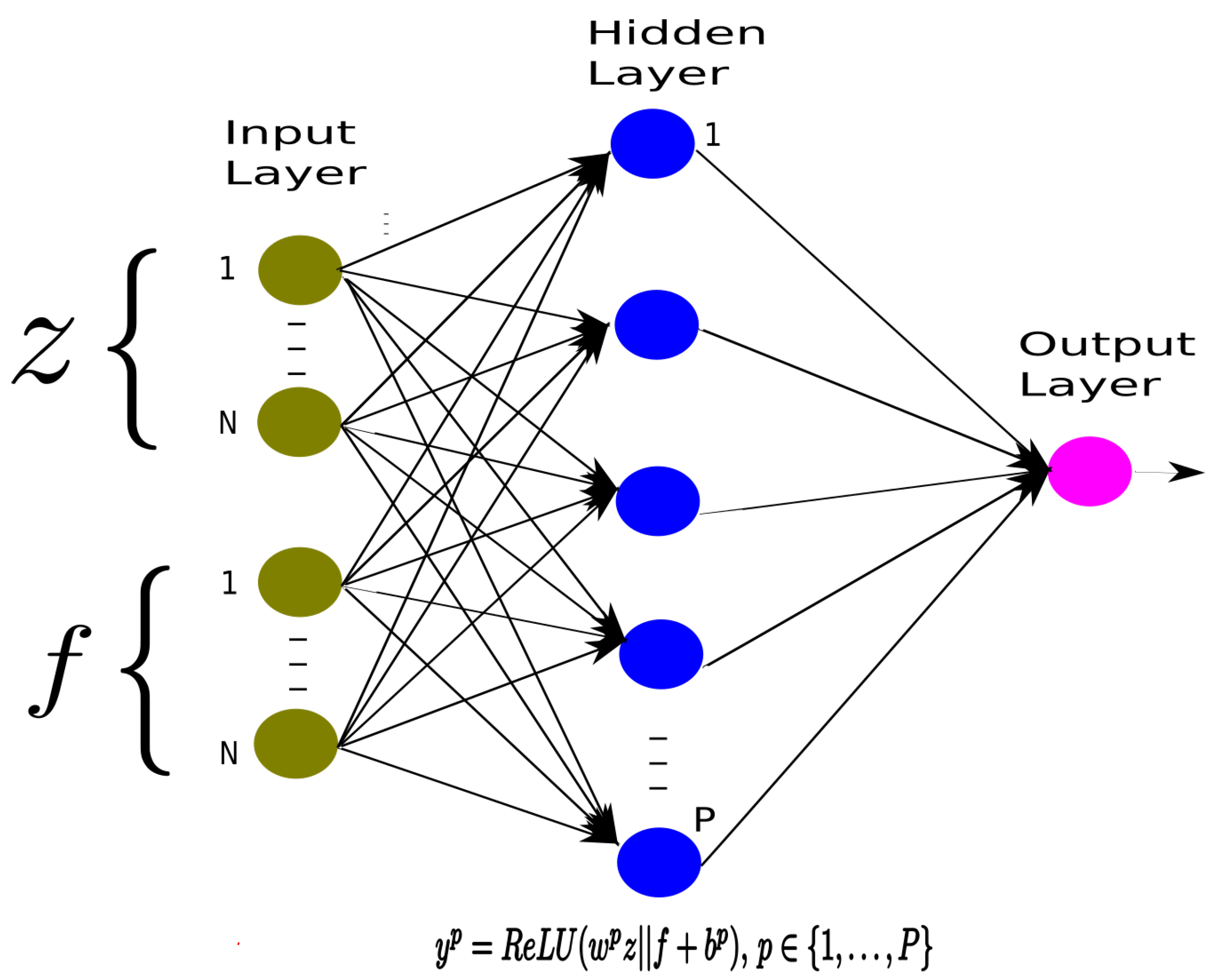
Figure 1 defines the architecture we implement for our DRL NN. The DRL NN has as input the vectors z and f, representing the customers’ delivery ordering and the ODs compensation vector; only one P hidden nodes layer with ReLU activation, and one linear output. Let ${\mathrm{w}}^{\mathrm{p}}\in {\mathrm{R}}^{2\mathrm{N}}$ represent the weights vector and ${\mathrm{b}}^{\mathrm{p}}\in \mathrm{R}$ the bias term for the p-th hidden node. We define ${\mathrm{w}}^{\mathrm{o}\mathrm{u}\mathrm{t}\mathrm{p}\mathrm{u}\mathrm{t}}\in {\mathrm{R}}^{\mathrm{P}}$ and ${\mathrm{b}}^{\mathrm{o}\mathrm{u}\mathrm{t}\mathrm{p}\mathrm{u}\mathrm{t}}\in \mathrm{R}$ analogously for the output layer.

For the DRL policy evaluation step, we now detail how cGAN data is dynamically generated and used within the Monte Carlo method. We note that the cGAN itself is trained as a previous step, using historical data, as part of the DRL algorithm. The cGAN is trained only once. By doing this, we train the cGAN’s generator model to generate a new sequence of scenarios based on previous scenarios and the compensation fee defined. The cGAN’s generator model is then used as part of the DRL policy evaluation step to dynamically generate a new sequence of scenarios for the execution of the Monte Carlo method at each iteration.

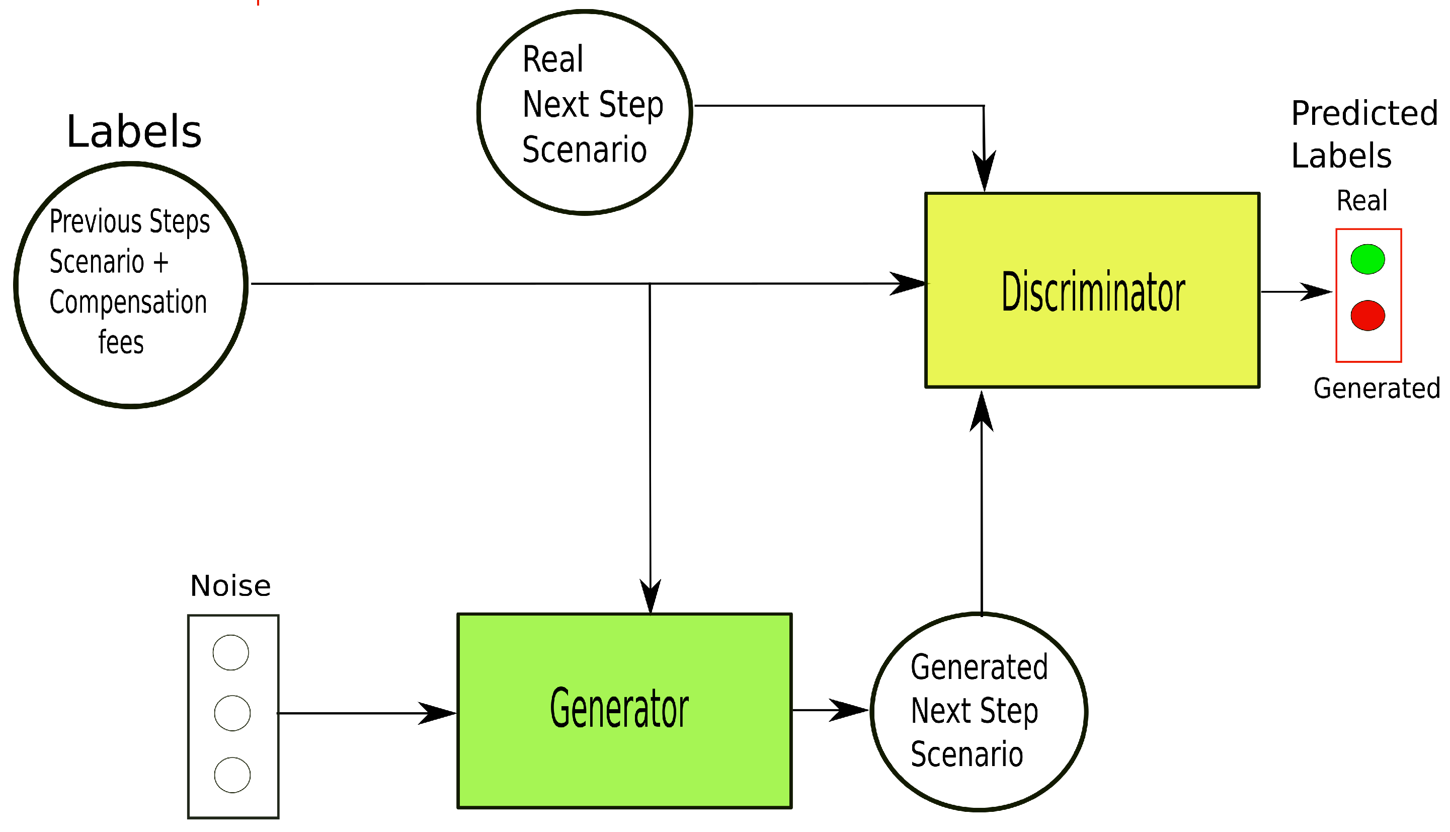
Figure 2 presents an overview of the cGAN. The cGAN englobes two neural networks, the generator and the discriminator. These NNs learn simultaneously in an adversarial process, with a two-player minimax game. First, we perform the conditioning by feeding the label representing the previous scenarios and compensation fees defined, into both the discriminator and generator as an additional input layer. The generator has the noise vector as input, which is sampled from a mean 0 and standard deviation 1 Gaussian distribution and forecasts ${\mathsf{\xi }}^{\mathrm{k}+1}$ with regard to the conditioning label. The discriminator has ${\mathsf{\xi }}^{\mathrm{k}+1}$ as input and verifies whether it is a valid value to follow the label or not. The discriminator is optimized to distinguish between generated data and real data.

The optimal generator NN models the probability distribution of ${\mathsf{\xi }}^{\mathrm{k}+1}$, conditioned to a label. In the end, information regarding any possible outcome can be extracted by sampling.

There are different ways to include conditional information in the neural network. Different approaches can be developed for how this information should be combined, or where in the network it should be included. Here, we include the label only in the input layer for the two networks and the representation data of the label is learned first by passing scenarios through a Long Short-Term Memory (LSTM) layer. LSTM neural networks, as introduced in [49], are distinguished by their “memory” as they take information from prior inputs to influence the current input and output.

The LSTM output is then concatenated with the compensation fee vector to finally compound the representation data.

Then, the noise vector, concatenated with the label is passed through two dense layers, leading to the predicted ${\mathsf{\xi }}^{\mathrm{k}+1}$ value. The discriminator inputs ${\mathsf{\xi }}^{\mathrm{k}+1}$ from the generator output or from the historical dataset concatenated with the label. This data passes a dense layer that outputs a single value specifying the output validity.

Our approach has to deal with a multivariate setting. In the multivariate setting, more complex NN architectures are needed to figure out dependencies between features. cGANs also require precise hyperparameter tuning to have a stable training process. It can be cumbersome to find adequate generator and discriminator architecture concurrently to perform adequately. To address this challenge we further adopt the cGAN training strategy of [44]. They build a probabilistic forecaster based on a deterministic forecaster using the GAN architecture. Namely, the generator model is based on the architecture and hyper- parameters of the deterministic forecaster. They search a generator and discriminator architecture separately, which results in the simplification of the architecture’s overall definition.

We now proceed with the policy improvement step of our DRL method. The $\mathsf{\tau }$-th policy improvement step involves solving the optimization problem related to (1), meaning that we find the first-stage decision to our problem that minimizes the expected total return expressed by the current approximation of the value function. Problem (1) is formulated as (see [32]):

$$min\sum _{\mathrm{p}=1}^{\mathrm{P}}{\mathrm{w}}_{\mathrm{p}}^{\mathrm{o}\mathrm{u}\mathrm{t}\mathrm{p}\mathrm{u}\mathrm{t}}{\mathrm{y}}^{\mathrm{p}}+{\mathrm{b}}^{\mathrm{o}\mathrm{u}\mathrm{t}\mathrm{p}\mathrm{u}\mathrm{t}}$$

(2)

$$\mathrm{s}.\mathrm{t}.{\mathrm{y}}^{\mathrm{p}}\ge \sum _{\mathrm{i}\in \{1,\dots ,\mathrm{N}\}}{\mathrm{w}}_{\mathrm{i}}^{\mathrm{p}}{\mathrm{z}}_{\mathrm{i}}+\sum _{\mathrm{i}\in \{\mathrm{N}+1,\dots ,2\mathrm{N}\}}{\mathrm{w}}_{\mathrm{i}}^{\mathrm{p}}{\mathrm{f}}_{\mathrm{i}}+{\mathrm{b}}^{\mathrm{p}}\forall 1\le \mathrm{p}\le \mathrm{P}$$

(3)

$${\mathrm{y}}^{\mathrm{p}}\le \sum _{\mathrm{i}\in \{1,\dots ,\mathrm{N}\}}{\mathrm{w}}_{\mathrm{i}}^{\mathrm{p}}{\mathrm{z}}_{\mathrm{i}}+\sum _{\mathrm{i}\in \{\mathrm{N}+1,\dots ,2\mathrm{N}\}}{\mathrm{w}}_{\mathrm{i}}^{\mathrm{p}}{\mathrm{f}}_{\mathrm{i}}+{\mathrm{b}}^{\mathrm{p}}+{\mathrm{M}}_{-}^{\mathrm{p}}(1-{\mathrm{s}}^{\mathrm{p}})\forall 1\le \mathrm{p}\le \mathrm{P}$$

(4)

$${\mathrm{y}}^{\mathrm{p}}\le {\mathrm{M}}_{+}^{\mathrm{p}}{\mathrm{s}}^{\mathrm{p}}\forall 1\le \mathrm{p}\le \mathrm{P}$$

(5)

$${\mathrm{y}}^{\mathrm{p}}\le \sum _{\mathrm{i}\in \mathrm{I},\mathrm{i}\le \mathrm{N}}{\mathrm{w}}_{\mathrm{i}}^{\mathrm{p}}{\mathrm{z}}_{\mathrm{i}}+\sum _{\mathrm{i}\in \mathrm{I},\mathrm{i}>\mathrm{N}}{\mathrm{w}}_{\mathrm{i}}^{\mathrm{p}}{\mathrm{f}}_{\mathrm{i}}-\sum _{\mathrm{i}\in \mathrm{I}}{\mathrm{w}}_{\mathrm{i}}^{\mathrm{p}}{\mathrm{L}}_{\mathrm{i}}^{\mathrm{p}}(1-{\mathrm{s}}^{\mathrm{p}})+({\mathrm{b}}^{\mathrm{p}}+\sum _{\mathrm{i}\notin \mathrm{I}}{\mathrm{w}}_{\mathrm{i}}^{\mathrm{p}}{\mathrm{U}}_{\mathrm{i}}^{\mathrm{p}}){\mathrm{s}}^{\mathrm{p}}\forall 1\le \mathrm{p}\le \mathrm{P},\mathrm{I}\subseteq \mathrm{s}\mathrm{u}\mathrm{p}\mathrm{p}({\mathrm{w}}^{\mathrm{p}})$$

(6)

$${\mathrm{x}}_{\mathrm{i}\mathrm{j}}+{\mathrm{x}}_{\mathrm{j}\mathrm{i}}=1\forall \mathrm{i},\mathrm{j}\in \mathrm{C},\mathrm{i}\ne \mathrm{j}$$

(7)

$${\mathrm{x}}_{\mathrm{i}\mathrm{j}}+{\mathrm{x}}_{\mathrm{j}\mathrm{k}}-{\mathrm{x}}_{\mathrm{i}\mathrm{k}}\le 1\forall \mathrm{i},\mathrm{k},\mathrm{j}\in \mathrm{C},\mathrm{i}\ne \mathrm{j}\ne \mathrm{k}$$

(8)

$${\displaystyle {\mathrm{z}}_{\mathrm{i}}=1+\sum _{\mathrm{j}\in \mathrm{V},\mathrm{j}\ne \mathrm{i}}{\mathrm{x}}_{\mathrm{j}\mathrm{i}}\forall \mathrm{i}\in \mathrm{C}}$$

(9)

$${\mathrm{f}}_{\mathrm{i}}^{\mathrm{m}\mathrm{i}\mathrm{n}}\le {\mathrm{f}}_{\mathrm{i}}\le {\mathrm{f}}_{\mathrm{i}}^{\mathrm{m}\mathrm{a}\mathrm{x}}\forall \mathrm{i}\in \mathrm{C}$$

(10)

$$\mathrm{z}\in {\mathbb{Z}}^{\mathrm{N}},\mathrm{f}\in {\mathbb{R}}^{\mathrm{N}},{\mathrm{y}}^{\mathrm{p}}\in \mathrm{R},{\mathrm{s}}^{\mathrm{p}}\in \{0,1\},\forall 1\le \mathrm{p}\le \mathrm{P},{\mathrm{x}}_{\mathrm{i}\mathrm{j}}\in \{0,1\}\forall \mathrm{i},\mathrm{j}\in \mathrm{C},\mathrm{i}\ne \mathrm{j}$$

(11)

where $\mathrm{s}\mathrm{u}\mathrm{p}\mathrm{p}(\mathrm{w})$ indicates the set of indices i such that ${\mathrm{w}}_{\mathrm{i}}\ne 0$ and components ${\mathrm{L}}_{\mathrm{i}}^{\mathrm{p}}$ and ${\mathrm{U}}_{\mathrm{i}}^{\mathrm{p}}$ are defined as

${\mathrm{L}}_{\mathrm{i}}^{\mathrm{p}}:=\left\{\begin{array}{cc}0,\hfill & {\mathrm{w}}_{\mathrm{i}}^{\mathrm{p}}\ge 0,\hfill \\ \mathrm{N}+1,\hfill & {\mathrm{w}}_{\mathrm{i}}^{\mathrm{p}}<0,\hfill \end{array}\right.$ $\mathrm{and}{\mathrm{U}}_{\mathrm{i}}^{\mathrm{p}}:=\left\{\begin{array}{cc}\mathrm{N}+1,\hfill & {\mathrm{w}}_{\mathrm{i}}^{\mathrm{p}}\ge 0,\hfill \\ 0,\hfill & {\mathrm{w}}_{\mathrm{i}}^{\mathrm{p}}<0,\hfill \end{array}\right.$

for $\mathrm{i}\le \mathrm{N}$ and

${\mathrm{L}}_{\mathrm{i}}^{\mathrm{p}}:=\left\{\begin{array}{cc}0,\hfill & {\mathrm{w}}_{\mathrm{i}}^{\mathrm{p}}\ge 0,\hfill \\ {\mathrm{f}}_{\mathrm{i}}^{\mathrm{m}\mathrm{a}\mathrm{x}}+1,\hfill & {\mathrm{w}}_{\mathrm{i}}^{\mathrm{p}}<0,\hfill \end{array}\right.$ $\mathrm{and}{\mathrm{U}}_{\mathrm{i}}^{\mathrm{p}}:=\left\{\begin{array}{cc}{\mathrm{f}}_{\mathrm{i}}^{\mathrm{m}\mathrm{a}\mathrm{x}}+1,\hfill & {\mathrm{w}}_{\mathrm{i}}^{\mathrm{p}}\ge 0,\hfill \\ 0,\hfill & {\mathrm{w}}_{\mathrm{i}}^{\mathrm{p}}<0,\hfill \end{array}\right.$

for $\mathrm{i}>\mathrm{N}$.

Formulation’s Big-Ms are set as ${\mathrm{M}}_{+}^{\mathrm{p}}={\displaystyle \underset{\mathrm{z}\in {\mathbb{Z}}^{\mathrm{N}},\mathrm{f}\in \mathrm{F}}{max}}{\mathrm{w}}^{\mathrm{p}}\mathrm{z}\left|\right|\mathrm{f}+{\mathrm{b}}^{\mathrm{p}}={\mathrm{w}}^{\mathrm{p}}{\mathrm{U}}^{\mathrm{p}}+{\mathrm{b}}^{\mathrm{p}}$ and ${\mathrm{M}}_{-}^{\mathrm{p}}={\displaystyle \underset{\mathrm{z}\in {\mathbb{Z}}^{\mathrm{N}},\mathrm{f}\in \mathrm{F}}{min}}{\mathrm{w}}^{\mathrm{p}}\mathrm{z}\left|\right|\mathrm{f}+{\mathrm{b}}^{\mathrm{p}}={\mathrm{w}}^{\mathrm{p}}{\mathrm{L}}^{\mathrm{p}}+{\mathrm{b}}^{\mathrm{p}}$, where $\mathrm{z}\left|\right|\mathrm{f}$ is the vector resulting from the concatenation of vectors z and f and ${\mathrm{w}}^{\mathrm{p}}\mathrm{z}\left|\right|\mathrm{f}$ is the inner product of vectors ${\mathrm{w}}^{\mathrm{p}}$ and $\mathrm{z}\left|\right|\mathrm{f}$. We define the N decision variables ${\mathrm{z}}_{\mathrm{i}}$, $1\le {\mathrm{z}}_{\mathrm{i}}\le \mathrm{N}$, giving the sequence in which customers will be delivered, a continuous variable ${\mathrm{f}}_{\mathrm{i}}$ defining the compensation paid for each customer outsourced, a continuous variable ${\mathrm{y}}^{\mathrm{p}}$ that models the output of the hidden node p and a binary variable ${\mathrm{s}}^{\mathrm{p}}$ that indicates whether the pre-activation function is positive or negative (i.e., whether the ReLU is active or not). We also introduce variables ${\mathrm{x}}_{\mathrm{i}\mathrm{j}}$ to define the delivery order: ${\mathrm{x}}_{\mathrm{i}\mathrm{j}}=1$ if customer i precedes customer j and 0 otherwise.

This pre-activation function is enforced by the “big-M ” constraints (4) and (5). The formulation is not polynomial in size, as there are exponentially many constraints of type (6), but these constraints simply strengthen the formulation.

Constraints (7) to (9) define the feasible region of all possible ordering of customers.

To be able to solve large instances and still have good solutions, we define a time limit of 1800 s to solve problem (1) at each policy improvement step and use the best solution provided until then. We apply warm start, callbacks to introduce lazy constraints and heuristics, and use only the needed half of ${\mathrm{x}}_{\mathrm{i}\mathrm{j}}$ variables, where $\mathrm{i}<\mathrm{j}$.

We warm start not only in an attempt to accelerate resolution but also to guarantee one incumbent solution. We adapt the Almost Nearest Neighbor Heuristic defined in the study of heuristic algorithms for the probabilistic TSP in [50], which considers independent marginals. We set a solution in an attempt to have a good feasible initial incumbent solution. The ordering of customers is defined by appending the customer with the lowest change in expected length from the last inserted customer to the tour. For a given set T of customers already inserted in a tour, inserting customer j with minimum cost is computed as

$$\begin{array}{c}\underset{\mathrm{j}\in \mathrm{C}\setminus \mathrm{T}}{\min }\sum _{\mathrm{i}=1}^{\left|\mathrm{T}\right|}(1-{\mathrm{m}}_{\mathrm{i}})(1-{\mathrm{m}}_{\mathrm{j}}){\mathrm{c}}_{\mathrm{i}\mathrm{j}}\prod _{\mathrm{k}=\mathrm{i}+1}^{\left|\mathrm{T}\right|}{\mathrm{m}}_{\mathrm{k}},\hfill \end{array}$$

where ${\mathrm{m}}_{\mathrm{i}},\mathrm{i}\in \mathrm{C}$ is the marginal Bernoulli probability of the component ${\mathsf{\xi }}_{\mathrm{i}},\mathrm{i}\in \mathrm{C}$ of the uncertain scenario vector given by the historical data. We also set ${\mathrm{f}}_{\mathrm{i}}={\mathrm{f}}_{\mathrm{i}}^{\mathrm{m}\mathrm{i}\mathrm{n}}, \forall \mathrm{i}\in \mathrm{C}$.

Constraints (6) are introduced as cutting planes by lazy constraints callbacks using a linear-time separation routine as described in [32]. Heuristics callbacks introduce simple heuristics by setting variables ${\mathrm{x}}_{\mathrm{i}\mathrm{j}}$ as binaries and following the same customer order given by the z relaxed solution.

Algorithm 1 summarizes the steps undertaken in our policy iteration algorithm.

Algorithm 1: Policy iteration algorithm

Initialize:     $\mathsf{\epsilon }\ge 0$     $\mathsf{\pi }\leftarrow$ an arbitrary $\mathsf{\epsilon }$-soft policy ${\mathsf{\pi }}_0$ with ${\mathrm{z}}_0,{\mathrm{f}}_0$   Train cGAN using scenarios historical data   $\mathrm{V}\mathrm{D}\leftarrow \varnothing$ Initialize empty dataset    Repeat for each policy iteration     Repeat for each episode:      Generate scenarios for episode using cGAN generator model       Generate an episode following $\mathsf{\pi }$: ${\mathsf{\xi }}^1,{\mathrm{a}}^1,{\mathrm{R}}^1,\dots ,{\mathsf{\xi }}^{\mathrm{K}},{\mathrm{a}}^{\mathrm{K}},{\mathrm{R}}^{\mathrm{K}}$       $\mathrm{T}\mathrm{R}\leftarrow 0$       Loop for each step of episode, $\mathrm{k}=\mathrm{K},\mathrm{K}-1,\dots ,1$:        $\mathrm{T}\mathrm{R}\leftarrow \mathrm{T}\mathrm{R}+{\mathrm{R}}^{\mathrm{k}}$        Append $\mathrm{T}\mathrm{R}$ to $\mathrm{R}\mathrm{e}\mathrm{t}\mathrm{u}\mathrm{r}\mathrm{n}\mathrm{s}(\mathrm{z},\mathrm{f})$        $\mathrm{V}\mathrm{D}(\mathrm{z},\mathrm{f})\leftarrow \mathrm{a}\mathrm{v}\mathrm{e}\mathrm{r}\mathrm{a}\mathrm{g}\mathrm{e}(\mathrm{R}\mathrm{e}\mathrm{t}\mathrm{u}\mathrm{r}\mathrm{n}\mathrm{s}(\mathrm{z},\mathrm{f}))$     Use VD to incrementally train the NN and approximate value function Va      ${\mathrm{z}}^{*},{\mathrm{f}}^{*}\leftarrow \mathrm{argmin}\mathrm{V}\mathrm{a}(\mathrm{z},\mathrm{f})$ using Va function MIP formulation     Define $\mathsf{\epsilon }$-soft policy $\mathsf{\pi }$ with ${\mathrm{z}}^{*},{\mathrm{f}}^{*}$

We define two forms for the reward calculation. Here, we want an optimal assignment of ODs. To perform this exactly we first formulate it as an optimization problem. The formulation for this problem is given as

$$min\sum _{\mathrm{i},\mathrm{j}\in \mathrm{V},\mathrm{i}\ne \mathrm{j}}{\mathrm{c}}_{\mathrm{i}\mathrm{j}}{\mathrm{x}}_{\mathrm{i}\mathrm{j}}+\sum _{\mathrm{i}\in \mathrm{C}}{\mathrm{f}}_{\mathrm{i}}{\mathrm{w}}_{\mathrm{i}}$$

$$\mathrm{s}.\mathrm{t}.\sum _{\mathrm{j}\in \mathrm{V},\mathrm{i}\ne \mathrm{j}}{\mathrm{x}}_{\mathrm{j}\mathrm{i}}=\sum _{\mathrm{j}\in \mathrm{V},\mathrm{i}\ne \mathrm{j}}{\mathrm{x}}_{\mathrm{i}\mathrm{j}}={\mathrm{v}}_{\mathrm{i}}\forall \mathrm{i}\in \mathrm{C}$$

(12)

$$\sum _{\mathrm{i}\in \mathrm{C}}{\mathrm{x}}_{\mathrm{i}0}-\sum _{\mathrm{i}\in \mathrm{C}}{\mathrm{x}}_{0\mathrm{i}}=0$$

(13)

$${\mathrm{v}}_{\mathrm{i}}+{\mathrm{w}}_{\mathrm{i}}\le 1\forall \mathrm{i}\in \mathrm{C}$$

(14)

$${\mathrm{v}}_{\mathrm{i}}+{\mathrm{w}}_{\mathrm{i}}\ge {\mathsf{\xi }}_{\mathrm{i}}\forall \mathrm{i}\in \mathrm{C}$$

(15)

$${\mathrm{w}}_{\mathrm{i}}\le {\mathsf{\xi }}_{\mathrm{i}}\forall \mathrm{i}\in \mathrm{C}$$

(16)

$${\mathrm{v}}_{\mathrm{i}}\le {\mathsf{\xi }}_{\mathrm{i}}\forall \mathrm{i}\in \mathrm{C}$$

(17)

$${\mathrm{w}}_{\mathrm{i}}\le {\mathsf{\xi }}_{\mathrm{i}+\mathrm{N}}\forall \mathrm{i}\in \mathrm{C}$$

(18)

$$\sum _{\mathrm{j}\in \mathrm{V},\mathrm{i}\ne \mathrm{j}}{\mathrm{y}}_{\mathrm{j}\mathrm{i}}-\sum _{\mathrm{j}\in \mathrm{V},\mathrm{i}\ne \mathrm{j}}{\mathrm{y}}_{\mathrm{i}\mathrm{j}}={\mathrm{v}}_{\mathrm{i}}\forall \mathrm{i}\in \mathrm{C}$$

(19)

$$\sum _{\mathrm{j}\in \mathrm{C}}{\mathrm{y}}_{0\mathrm{j}}=\sum _{\mathrm{j}\in \mathrm{C}}{\mathrm{v}}_{\mathrm{j}}$$

(20)

$${\mathrm{y}}_{\mathrm{i}0}=0\forall \mathrm{i}\in \mathrm{C}$$

(21)

$${\mathrm{y}}_{\mathrm{i}\mathrm{j}}\le \mathrm{Q}{\mathrm{x}}_{\mathrm{i}\mathrm{j}}\forall \mathrm{i},\mathrm{j}\in \mathrm{V},\mathrm{i}\ne \mathrm{j}$$

(22)

$$\sum _{\mathrm{j}\in \mathrm{V},\mathrm{i}\ne \mathrm{j}}{\mathrm{t}}_{\mathrm{i}\mathrm{j}}-\sum _{\mathrm{j}\in \mathrm{V},\mathrm{i}\ne \mathrm{j}}{\mathrm{t}}_{\mathrm{j}\mathrm{i}}=\sum _{\mathrm{j}\in \mathrm{V},\mathrm{i}\ne \mathrm{j}}{\mathrm{d}}_{\mathrm{i}\mathrm{j}}{\mathrm{x}}_{\mathrm{i}\mathrm{j}}\forall \mathrm{i}\in \mathrm{C}$$

(23)

$${\mathrm{t}}_{0\mathrm{i}}\ge {\mathrm{d}}_{0\mathrm{i}}{\mathrm{x}}_{0\mathrm{i}}\forall \mathrm{i}\in \mathrm{C}$$

(24)

$${\mathrm{t}}_{\mathrm{i}\mathrm{j}}\le (\mathrm{D}-{\mathrm{d}}_{\mathrm{j}0}){\mathrm{x}}_{\mathrm{i}\mathrm{j}}\forall \mathrm{i},\mathrm{j}\in \mathrm{V},\mathrm{i}\ne \mathrm{j}$$

(25)

$$\sum _{\mathrm{j}\in \mathrm{S}}{\mathrm{x}}_{\mathrm{i}\mathrm{j}}=0\forall \mathrm{i}\in \mathrm{C},\mathrm{S}=\{\mathrm{j}|{\mathrm{z}}_{\mathrm{j}}<{\mathrm{z}}_{\mathrm{i}}\}$$

(26)

$$\sum _{\mathrm{j}\in \mathrm{S}}{\mathrm{x}}_{\mathrm{j}\mathrm{i}}\le {\mathrm{v}}_{\mathrm{i}}\forall \mathrm{i}\in \mathrm{C};\mathrm{S}=\{\mathrm{j}|{\mathrm{z}}_{\mathrm{j}}<{\mathrm{z}}_{\mathrm{i}}]\}$$

(27)

$${\mathrm{x}}_{\mathrm{i}\mathrm{j}}\in \{0,1\}\forall \mathrm{i},\mathrm{j}\in \mathrm{V},\mathrm{i}\ne \mathrm{j},{\mathrm{y}}_{\mathrm{i}\mathrm{j}},{\mathrm{t}}_{\mathrm{i}\mathrm{j}}\ge 0\forall \mathrm{i},\mathrm{j}\in \mathrm{V},\mathrm{i}\ne \mathrm{j}$$

(28)

$${\mathrm{w}}_{\mathrm{i}}\in \{0,1\}{\mathrm{v}}_{\mathrm{i}}\in \{0,1\}\forall \mathrm{i}\in \mathrm{C}$$

(29)

where we define variables ${\mathrm{x}}_{\mathrm{i}\mathrm{j}}$ = 1 if customer i is served by a vehicle right before j, 0 otherwise, ${\mathrm{w}}_{\mathrm{i}}$ = 1 if customer i is served by an OD, 0 otherwise, ${\mathrm{v}}_{\mathrm{i}}$ = 1 if customer i is served by a vehicle, 0 otherwise, ${\mathrm{y}}_{\mathrm{i}\mathrm{j}}$ as the accumulated capacity loaded between customer i and j and ${\mathrm{t}}_{\mathrm{i}\mathrm{j}}$ as the accumulated time spent between customer i and j. The objective is to minimize the total cost of routes plus OD payments. Constraints (12) and (13) are route flow conservation and should be considered every time a customer is included in a route, ${\mathrm{v}}_{\mathrm{i}}=1$. Constraints (14) define that customer i is served by a vehicle, or an OD or none. Constraints (15) define that customer i is served by a vehicle or an OD if ${\mathsf{\xi }}_{\mathrm{i}}=1$. Constraints (16) and (17) define that customer i is not served by an OD or a vehicle if ${\mathsf{\xi }}_{\mathrm{i}}=0$. Constraints (18) define that customer i is served by an OD only if an OD is available. Constraints (19) to (22) define the capacity restrictions. Constraints (23) to (25) define the time duration restrictions. Constraints (26) and (27) guarantee that the order of first-stage decision z is respected. Here, z, f and $\mathsf{\xi }$ are data input to the problem. For our algorithms, we define a time limit of 600 s to solve the problem relative to this formulation and use the best solution provided until then.

As an alternative, we provide a heuristic for reward calculation where the condition to reduce cost by OD assignment is verified only locally. By Algorithm 2, customers are allocated to ODs only if the corresponding OD compensation fee is less than the vehicle cost to route from the previous to the next available customer (customers with delivery orders in the scenario being referenced).    

Algorithm 2: Reward function for variant 2 of recourse model

Initialize:   $\mathrm{l}\mathrm{a}\mathrm{s}\mathrm{t}\mathrm{s}\mathrm{t}\mathrm{o}\mathrm{p}=0$; depot   $\mathrm{c}\mathrm{o}\mathrm{s}\mathrm{t}=0$; cost of vehicles route   $\mathrm{c}\mathrm{a}\mathrm{p}=0$; accumulated capacity of a vehicle   $\mathrm{t}\mathrm{i}\mathrm{m}\mathrm{e}=0$; accumulated time duration of a vehicle route   $\mathrm{c}\mathrm{o}\mathrm{n}\mathrm{t}\mathrm{i}\mathrm{n}\mathrm{u}\mathrm{e}=\mathrm{t}\mathrm{r}\mathrm{u}\mathrm{e}$; define when to stop algorithm   $\mathrm{b}\mathrm{y}\mathrm{p}\mathrm{a}\mathrm{s}\mathrm{s}=\mathrm{f}\mathrm{a}\mathrm{l}\mathrm{s}\mathrm{e}$; should bypass OD available   $\mathrm{i}=0$   while continue     $\mathrm{i}+=1$      if $\mathsf{\xi }[{\mathrm{z}}^{-1}[\mathrm{i}]]==1$ and $(\mathsf{\xi }[\mathrm{N}+{\mathrm{z}}^{-1}[\mathrm{i}]]==0$ or $\mathrm{b}\mathrm{y}\mathrm{p}\mathrm{a}\mathrm{s}\mathrm{s})$        $\mathrm{b}\mathrm{y}\mathrm{p}\mathrm{a}\mathrm{s}\mathrm{s}=\mathrm{f}\mathrm{a}\mathrm{l}\mathrm{s}\mathrm{e}$         if $\mathrm{t}\mathrm{i}\mathrm{m}\mathrm{e}+\mathrm{d}[\mathrm{l}\mathrm{a}\mathrm{s}\mathrm{t}\mathrm{s}\mathrm{t}\mathrm{o}\mathrm{p},{\mathrm{z}}^{-1}[\mathrm{i}]]+\mathrm{d}[{\mathrm{z}}^{-1}[\mathrm{i}],\mathrm{d}\mathrm{e}\mathrm{p}\mathrm{o}\mathrm{t}]\le \mathrm{t}\mathrm{i}\mathrm{m}\mathrm{e}\mathrm{l}\mathrm{i}\mathrm{m}\mathrm{i}\mathrm{t}$          $\mathrm{c}\mathrm{o}\mathrm{s}\mathrm{t}+=\mathrm{c}[\mathrm{l}\mathrm{a}\mathrm{s}\mathrm{t}\mathrm{s}\mathrm{t}\mathrm{o}\mathrm{p},{\mathrm{z}}^{-1}[\mathrm{i}]];\mathrm{t}\mathrm{i}\mathrm{m}\mathrm{e}+=\mathrm{d}[\mathrm{l}\mathrm{a}\mathrm{s}\mathrm{t}\mathrm{s}\mathrm{t}\mathrm{o}\mathrm{p},{\mathrm{z}}^{-1}[\mathrm{i}]]$          $\mathrm{l}\mathrm{a}\mathrm{s}\mathrm{t}\mathrm{s}\mathrm{t}\mathrm{o}\mathrm{p}={\mathrm{z}}^{-1}[\mathrm{i}];\mathrm{c}\mathrm{a}\mathrm{p}+=1$          if $\mathrm{i}==\mathrm{N}$           $\mathrm{c}\mathrm{o}\mathrm{s}\mathrm{t}+=\mathrm{c}[{\mathrm{z}}^{-1}[\mathrm{i}],\mathrm{d}\mathrm{e}\mathrm{p}\mathrm{o}\mathrm{t}];\mathrm{c}\mathrm{o}\mathrm{n}\mathrm{t}\mathrm{i}\mathrm{n}\mathrm{u}\mathrm{e}=\mathrm{f}\mathrm{a}\mathrm{l}\mathrm{s}\mathrm{e}$          elseif cap == Q           $\mathrm{c}\mathrm{o}\mathrm{s}\mathrm{t}+=\mathrm{c}[\mathrm{l}\mathrm{a}\mathrm{s}\mathrm{t}\mathrm{s}\mathrm{t}\mathrm{o}\mathrm{p},\mathrm{d}\mathrm{e}\mathrm{p}\mathrm{o}\mathrm{t}];\mathrm{l}\mathrm{a}\mathrm{s}\mathrm{t}\mathrm{s}\mathrm{t}\mathrm{o}\mathrm{p}=\mathrm{d}\mathrm{e}\mathrm{p}\mathrm{o}\mathrm{t};\mathrm{c}\mathrm{a}\mathrm{p}=0;\mathrm{t}\mathrm{i}\mathrm{m}\mathrm{e}=0$         else          if $\mathrm{i}==\mathrm{N}\#$ assume 2*time from depot to $\mathrm{i}\le$ timelimit always           $\mathrm{c}\mathrm{o}\mathrm{s}\mathrm{t}+=\mathrm{c}[\mathrm{l}\mathrm{a}\mathrm{s}\mathrm{t}\mathrm{s}\mathrm{t}\mathrm{o}\mathrm{p},\mathrm{d}\mathrm{e}\mathrm{p}\mathrm{o}\mathrm{t}]+\mathrm{c}[\mathrm{d}\mathrm{e}\mathrm{p}\mathrm{o}\mathrm{t},{\mathrm{z}}^{-1}[\mathrm{i}]]+\mathrm{c}[{\mathrm{z}}^{-1}[\mathrm{i}],\mathrm{d}\mathrm{e}\mathrm{p}\mathrm{o}\mathrm{t}]$           $\mathrm{c}\mathrm{o}\mathrm{n}\mathrm{t}\mathrm{i}\mathrm{n}\mathrm{u}\mathrm{e}=\mathrm{f}\mathrm{a}\mathrm{l}\mathrm{s}\mathrm{e}$          else           $\mathrm{c}\mathrm{o}\mathrm{s}\mathrm{t}+=\mathrm{c}[\mathrm{l}\mathrm{a}\mathrm{s}\mathrm{t}\mathrm{s}\mathrm{t}\mathrm{o}\mathrm{p},\mathrm{d}\mathrm{e}\mathrm{p}\mathrm{o}\mathrm{t}]+\mathrm{c}[\mathrm{d}\mathrm{e}\mathrm{p}\mathrm{o}\mathrm{t},{\mathrm{z}}^{-1}[\mathrm{i}]]$           $\mathrm{t}\mathrm{i}\mathrm{m}\mathrm{e}=\mathrm{d}[\mathrm{d}\mathrm{e}\mathrm{p}\mathrm{o}\mathrm{t},{\mathrm{z}}^{-1}[\mathrm{i}]];\mathrm{l}\mathrm{a}\mathrm{s}\mathrm{t}\mathrm{s}\mathrm{t}\mathrm{o}\mathrm{p}={\mathrm{z}}^{-1}[\mathrm{i}]];\mathrm{c}\mathrm{a}\mathrm{p}=1$      elseif $\mathsf{\xi }[{\mathrm{z}}^{-1}[\mathrm{i}]]==1$ and $\mathsf{\xi }[{\mathrm{z}}^{-1}[\mathrm{i}]+\mathrm{N}]==1$      $\#$ find next customer available      $\mathrm{j}=\mathrm{i}+1$         while $\mathrm{j}\le \mathrm{N}$ and $\mathsf{\xi }[{\mathrm{z}}^{-1}[\mathrm{j}]]==0)$           $\mathrm{j}+=1$         if $\mathrm{j}\le \mathrm{N}$ and $\mathrm{f}[{\mathrm{z}}^{-1}[\mathrm{i}]]\le \mathrm{c}[\mathrm{l}\mathrm{a}\mathrm{s}\mathrm{t}\mathrm{s}\mathrm{t}\mathrm{o}\mathrm{p},{\mathrm{z}}^{-1}[\mathrm{i}]]+\mathrm{c}[{\mathrm{z}}^{-1}[\mathrm{i}],{\mathrm{z}}^{-1}[\mathrm{j}]]$          $\mathrm{c}\mathrm{o}\mathrm{s}\mathrm{t}+=\mathrm{f}[{\mathrm{z}}^{-1}[\mathrm{i}]]$          $\mathrm{i}=\mathrm{j}-1$         elseif $\mathrm{j}>\mathrm{N}$ and $\mathrm{f}[{\mathrm{z}}^{-1}[\mathrm{i}]]\le \mathrm{c}[\mathrm{l}\mathrm{a}\mathrm{s}\mathrm{t}\mathrm{s}\mathrm{t}\mathrm{o}\mathrm{p},{\mathrm{z}}^{-1}[\mathrm{i}]]+\mathrm{c}[{\mathrm{z}}^{-1}[\mathrm{i}],\mathrm{d}\mathrm{e}\mathrm{p}\mathrm{o}\mathrm{t}]$          $\mathrm{c}\mathrm{o}\mathrm{n}\mathrm{t}\mathrm{i}\mathrm{n}\mathrm{u}\mathrm{e}=\mathrm{f}\mathrm{a}\mathrm{l}\mathrm{s}\mathrm{e}$          $\mathrm{c}\mathrm{o}\mathrm{s}\mathrm{t}+=\mathrm{f}[{\mathrm{z}}^{-1}[\mathrm{i}]]$         if $\mathrm{c}\mathrm{a}\mathrm{p}\ne 0$          $\mathrm{c}\mathrm{o}\mathrm{s}\mathrm{t}+=\mathrm{c}[\mathrm{l}\mathrm{a}\mathrm{s}\mathrm{t}\mathrm{s}\mathrm{t}\mathrm{o}\mathrm{p},\mathrm{d}\mathrm{e}\mathrm{p}\mathrm{o}\mathrm{t}]$         elseif $\mathrm{j}\le \mathrm{N}$ and $\mathrm{f}[{\mathrm{z}}^{-1}[\mathrm{i}]]>\mathrm{c}[\mathrm{l}\mathrm{a}\mathrm{s}\mathrm{t}\mathrm{s}\mathrm{t}\mathrm{o}\mathrm{p},{\mathrm{z}}^{-1}[\mathrm{i}]]+\mathrm{c}[{\mathrm{z}}^{-1}[\mathrm{i}],{\mathrm{z}}^{-1}[\mathrm{j}]]$           $\mathrm{b}\mathrm{y}\mathrm{p}\mathrm{a}\mathrm{s}\mathrm{s}=\mathrm{t}\mathrm{r}\mathrm{u}\mathrm{e};\mathrm{i}-=1$         elseif $\mathrm{j}>\mathrm{N}$ and $\mathrm{f}[{\mathrm{z}}^{-1}[\mathrm{i}]]\le \mathrm{c}[\mathrm{l}\mathrm{a}\mathrm{s}\mathrm{t}\mathrm{s}\mathrm{t}\mathrm{o}\mathrm{p},{\mathrm{z}}^{-1}[\mathrm{i}]]+\mathrm{c}[{\mathrm{z}}^{-1}[\mathrm{i}],\mathrm{d}\mathrm{e}\mathrm{p}\mathrm{o}\mathrm{t}]$           $\mathrm{b}\mathrm{y}\mathrm{p}\mathrm{a}\mathrm{s}\mathrm{s}=\mathrm{t}\mathrm{r}\mathrm{u}\mathrm{e};\mathrm{i}-=1$       else          if $\mathrm{i}==\mathrm{N}\mathrm{and}\mathrm{c}\mathrm{a}\mathrm{p}\ne 0$           $\mathrm{c}\mathrm{o}\mathrm{s}\mathrm{t}+=\mathrm{c}[\mathrm{l}\mathrm{a}\mathrm{s}\mathrm{t}\mathrm{s}\mathrm{t}\mathrm{o}\mathrm{p},\mathrm{d}\mathrm{e}\mathrm{p}\mathrm{o}\mathrm{t}]$          if $\mathrm{i}==\mathrm{N}$           $\mathrm{c}\mathrm{o}\mathrm{n}\mathrm{t}\mathrm{i}\mathrm{n}\mathrm{u}\mathrm{e}=\mathrm{f}\mathrm{a}\mathrm{l}\mathrm{s}\mathrm{e}$

5. Experiments and Computational Results

The experiments have a three-fold objective: (1) analyze the effect of considering a flexible compensation scheme from a solution improvement perspective; (2) analyze the sensitivity of the algorithm’s solution to key parameters; and (3) analyze the performance of the algorithms we have implemented.

To pursue this objective, we present in the sections below, the instances setting and the implemented benchmark algorithms.

Algorithms were developed in Python, with Keras, Tensorflow, and Docplex integrated with Cplex 12.9, running with a machine with 16 GB of RAM and Intel I7 CPU at 2.30 GHz. We present key parameters and additional architectural features defined for the DRL algorithm and used in the experiment:

• We define key parameters with default values: number of nodes of the hidden layer of the NN as 16, number of policy iterations as 15, number of historical scenarios in sequence for cGAN as 1500 and number of scenarios generated by cGAN for DRL Monte Carlo Simulation as 800,000. For some of the experiments, when specified, we change default values to analyze the sensitivity of the DRL method to these changes.
• Exploration and exploitation during training are performed by setting $\mathsf{\epsilon }$-soft policies. We set the probability of exploring $\mathsf{\epsilon }=0.6$ and exploiting $1-\mathsf{\epsilon }$ and decay $\mathsf{\epsilon }$ over the policy iterations.
• We apply a learning rate with an exponential decay from 0.01 with the base 0.96 and the decay rate 1/6000 for updating weights.
• We pass through the entire episodes dataset 100 times (epochs) with a batch size of 100.

5.1. Instances

We generate random test instances having $\left|\mathrm{C}\right|+1$ vertices (depot and $\left|\mathrm{C}\right|$ customers) for different values of $\left|\mathrm{C}\right|\in \{10,30,70,150,300\}$. Five instances for each number of customers are generated. Results indicated by the number of customers are an average of the results of all their associated instances.

Customers’ locations for each instance are assigned randomly from a grid of 100 × 100 possible locations. We assume that travel times and costs are deterministic and proportional to the euclidean distances between customers.

The compensation fee limits ${\mathrm{f}}_{\mathrm{i}}^{\mathrm{m}\mathrm{i}\mathrm{n}}$ and ${\mathrm{f}}_{\mathrm{i}}^{\mathrm{m}\mathrm{a}\mathrm{x}}$ for each customer i are set to the minimal and maximal detour considering all pairs of customers $\mathrm{r},\mathrm{j}\in \mathrm{C},\mathrm{i}\ne \mathrm{j}\ne \mathrm{r}$ plus a small value ${\mathrm{f}}^{\mathrm{f}\mathrm{i}\mathrm{x}\mathrm{e}\mathrm{d}}$, to avoid zero compensations, and given by ${\displaystyle {\mathrm{f}}_{\mathrm{i}}^{\mathrm{m}\mathrm{i}\mathrm{n}}={\mathrm{f}}^{\mathrm{f}\mathrm{i}\mathrm{x}\mathrm{e}\mathrm{d}}+\underset{\mathrm{j},\mathrm{r}\in \mathrm{C}}{min}{\mathrm{c}}_{\mathrm{j}\mathrm{i}}+{\mathrm{c}}_{\mathrm{i}\mathrm{r}}-{\mathrm{c}}_{\mathrm{j}\mathrm{r}}}$ and ${\displaystyle {\mathrm{f}}_{\mathrm{i}}^{\mathrm{m}\mathrm{a}\mathrm{x}}={\mathrm{f}}^{\mathrm{f}\mathrm{i}\mathrm{x}\mathrm{e}\mathrm{d}}+\underset{\mathrm{j},\mathrm{r}\in \mathrm{C}}{max}{\mathrm{c}}_{\mathrm{j}\mathrm{i}}+{\mathrm{c}}_{\mathrm{i}\mathrm{r}}-{\mathrm{c}}_{\mathrm{j}\mathrm{r}}}$.

Customers’ orders and OD availability occur randomly around the day and present themselves for each time window as scenarios. We assume there is a sequence of scenarios, conditioned by compensation fee, available as data and that is sufficient to train the cGAN.

We artificially generate these scenarios for our test instances based on two probability vectors that define for each customer $\mathrm{i}\in \mathrm{C}$, a marginal probability ${\mathrm{m}}_{\mathrm{i}}$ for his/her order, and a marginal probability ${\mathrm{o}}_{\mathrm{i}}$ for the availability of an OD to attend him/her. The marginal probability ${\mathrm{o}}_{\mathrm{i}}$ is dependent on the compensation fee ${\mathrm{f}}_{\mathrm{i}}$, defined as a pair $({\mathrm{o}}_{\mathrm{i}},{\mathrm{f}}_{\mathrm{i}})$.

To assure scenario consistency, the OD availability is only assigned when the respective customer is also assigned to a delivery order. To introduce a correlation between scenarios we force customers to have a maximum of one delivery order per day. We generate 1500 scenarios that are used to train the cGAN, plus 1500 scenarios that are used to simulate the solutions provided by the algorithms (out-of-sample performance). Note that the cGAN 1500 scenarios generated to simulate the solutions are, as always with the cGAN, conditioned for the compensation fees defined as first-stage solutions.

We assume that the pairs $({\mathrm{o}}_{\mathrm{i}},{\mathrm{f}}_{\mathrm{i}})$ generated are coherent, in the sense that the compensation fee influences the probability of an OD accepting to outsource.

The values ${\mathrm{m}}_{\mathrm{i}}$ are assigned randomly for each instance in a range smaller than 0.3.

We set three values for ${\mathrm{f}}_{\mathrm{i}}$, ${\mathrm{f}}_{\mathrm{i}}={\mathrm{f}}_{\mathrm{i}}^{\mathrm{m}\mathrm{i}\mathrm{n}}$, ${\mathrm{f}}_{\mathrm{i}}={\mathrm{f}}_{\mathrm{i}}^{\mathrm{m}\mathrm{a}\mathrm{x}}$, ${\mathrm{f}}_{\mathrm{i}}=({\mathrm{f}}_{\mathrm{i}}^{\mathrm{m}\mathrm{a}\mathrm{x}}-{\mathrm{f}}_{\mathrm{i}}^{\mathrm{m}\mathrm{i}\mathrm{n}})/2+{\mathrm{f}}_{\mathrm{i}}^{\mathrm{m}\mathrm{i}\mathrm{n}}$. The values of ${\mathrm{o}}_{\mathrm{i}}$ are assigned randomly for each instance, according to the values of ${\mathrm{f}}_{\mathrm{i}}$. If ${\mathrm{f}}_{\mathrm{i}}={\mathrm{f}}_{\mathrm{i}}^{\mathrm{m}\mathrm{i}\mathrm{n}}$, then ${\mathrm{o}}_{\mathrm{i}}$ is assigned in a range smaller than 0.1. If ${\mathrm{f}}_{\mathrm{i}}={\mathrm{f}}_{\mathrm{i}}^{\mathrm{m}\mathrm{a}\mathrm{x}}$, then ${\mathrm{o}}_{\mathrm{i}}$ is assigned in a range greater than 0.3. If ${\mathrm{f}}_{\mathrm{i}}={\mathrm{f}}_{\mathrm{i}}^{\mathrm{m}\mathrm{a}\mathrm{x}}$, ${\mathrm{f}}_{\mathrm{i}}=({\mathrm{f}}_{\mathrm{i}}^{\mathrm{m}\mathrm{a}\mathrm{x}}-{\mathrm{f}}_{\mathrm{i}}^{\mathrm{m}\mathrm{i}\mathrm{n}})/2+{\mathrm{f}}_{\mathrm{i}}^{\mathrm{m}\mathrm{i}\mathrm{n}}$, then ${\mathrm{o}}_{\mathrm{i}}$ is assigned in a range between 0.1 and 0.3.

Each episode is composed of a delivery day with four time windows of 2 h each, and therefore, four scenarios.

The professional fleet vehicle capacity is set to $\mathrm{Q}=\lfloor \frac{\left|\mathrm{C}\right|}{3}\rfloor$ and the time limit of a route is given by the time windows of 2 h.

5.2. Benchmark Algorithms

We present in

Table 1. Algorithms

Algorithm Code	Description
$\mathrm{D}\mathrm{R}\mathrm{L}\mathrm{V}1$	The DRL method presented in Section 4 with exact recourse
$\mathrm{D}\mathrm{R}\mathrm{L}\mathrm{V}2$	The DRL method presented in Section 4 with heuristic recourse
$\mathrm{D}\mathrm{R}\mathrm{L}\mathrm{F}$	The DRL method with Compensation fee fixed and set to minimum

a general description of the different algorithms we run our instances with.

Besides implementing algorithms $\mathrm{D}\mathrm{R}\mathrm{L}\mathrm{V}1$ and $\mathrm{D}\mathrm{R}\mathrm{L}\mathrm{V}2$ for the methods presented in Section 4, we implement algorithm $\mathrm{D}\mathrm{R}\mathrm{L}\mathrm{F}$ to run the same instances. $\mathrm{D}\mathrm{R}\mathrm{L}\mathrm{F}$ is the algorithm developed in [11] for the heuristic recourse. The difference is that the compensation fees are not a decision to be made. They are fixed and set to ${\mathrm{f}}_{\mathrm{i}}^{\mathrm{m}\mathrm{i}\mathrm{n}},\forall \mathrm{i}\in \mathrm{C}$. $\mathrm{D}\mathrm{R}\mathrm{L}\mathrm{F}$ was implemented to allow us to verify the power of flexible compensation for our instances, running with the other algorithms.

5.3. Initial Insights

We start by gaining qualitative insights into the potential benefits of different compensation levels for crowdshipping the last-mile delivery. We want to understand the sensitivity to problem characteristics and for this, we analyze some specific toy instances.

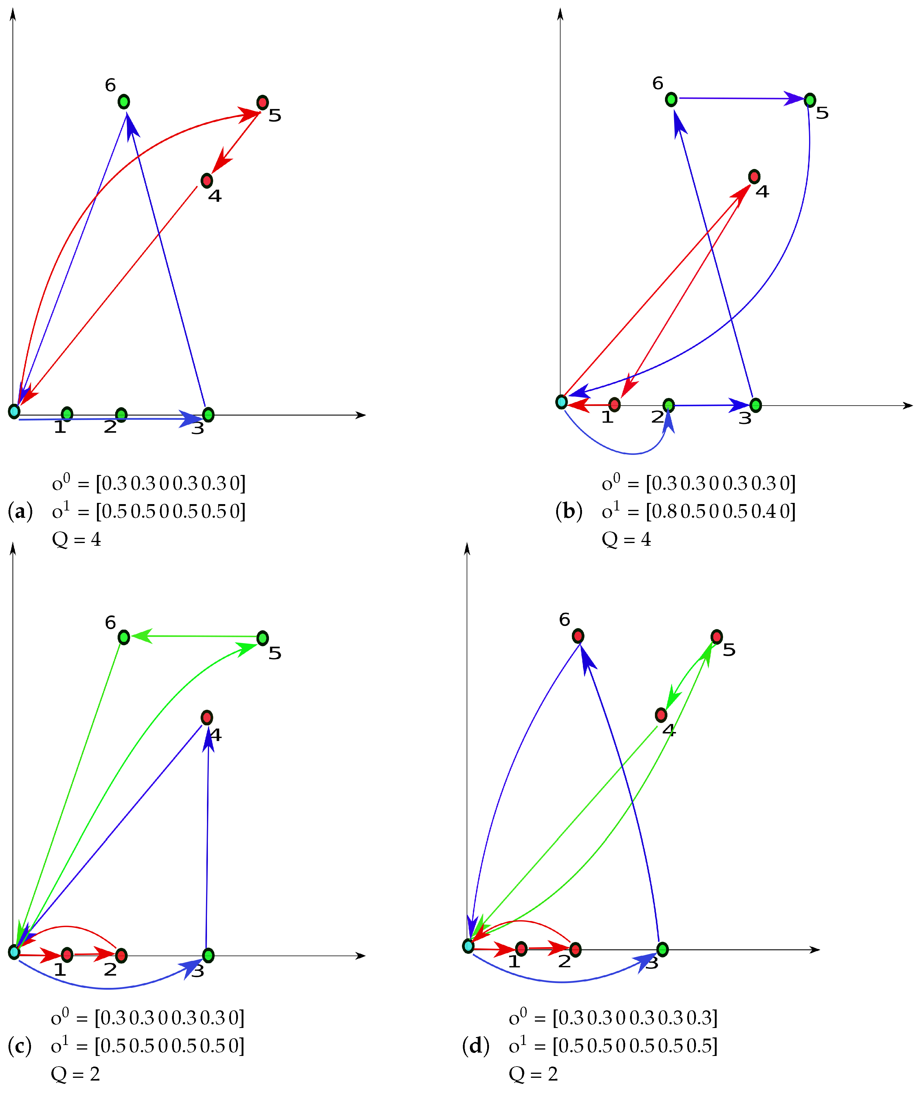
Figure 3 presents four instances indicating six customers’ positions in a graph, the best-constructed routes defined for a scenario where all customers have online orders and no ODs available, and what level of compensation was paid for each customer being outsourced, as in the solution of our $\mathrm{D}\mathrm{R}\mathrm{L}\mathrm{V}1$ algorithm.

For these toy examples, we assume there exist only two levels of compensation, ${\mathrm{f}}^0$, for the lower level, and ${\mathrm{f}}^1$ for the higher level. For compensation fees ${\mathrm{f}}_0$ and ${\mathrm{f}}_1$, we assume the scenarios follow a distribution probability where the Bernoulli marginals of elements ${\mathsf{\xi }}_{\mathrm{i}}=1,\mathrm{i}\in \mathrm{C},\mathrm{i}\le \mathrm{N}$ are equal to 100 %, and the Bernoulli marginals of elements ${\mathsf{\xi }}_{\mathrm{i}}=1,\mathrm{i}\in \mathrm{C},\mathrm{i}>\mathrm{N}$ are equal to ${\mathrm{o}}^0$ and ${\mathrm{o}}^1$, respectively.

The level of compensation paid for each instance is indicated by the color given to the customer location in the graph, referenced by axes, being red for the higher level of compensation and green for the lower level. The depot is located at the origin of the axes. Each route is indicated also by arrows in different colors.

Below each graph, we indicate the assumptions made for vectors ${\mathrm{o}}^0$, ${\mathrm{o}}^1$, and capacity Q.

Our exercise here is to verify how the solution (routes and level of compensation) changes with the assumptions of ${\mathrm{o}}^0$, ${\mathrm{o}}^1$, ${\mathrm{f}}^0$, ${\mathrm{f}}^1$, and Q.

In Figure 3a customers 3 and 6 are fixed to be delivered by the professional fleet (${\mathrm{o}}_3^0={\mathrm{o}}_3^1={\mathrm{o}}_6^0={\mathrm{o}}_6^1=0$). Since in this case $\mathrm{Q}=4$, the solution creates only two routes and leaves the two fixed customers to be delivered in sequence. We note that, since in this instance, a straight path between the depot and customer 3 can always be performed including customers 1 and 2 with no extra cost, then it was not worth offering customers 1 and 2 a higher compensation fee.

The instance in Figure 3b has the same assumptions as in Figure 3a, except that now, for the same ${\mathrm{f}}^1$ we increase the probability ${\mathrm{o}}_1^1$ and decrease ${\mathrm{o}}_5^1$. A naive expectation would be that, in this case, it would continue not to be worth paying extra for customer 1 since we have a straight path to customer 3 still. Different from that, the algorithm is now able to change the route solution and will pay extra for another set of two customers only.

Now in Figure 3c, we also replicate assumptions of Figure 3a, except the capacity $\mathrm{Q}=2$. We see that, in this case, three customers are selected to pay extra instead of two, and the route including in sequence customers 1, 2, and 3 is not worth it anymore due to restrictions in vehicle capacity.

For Figure 3d, we just change the assumption of instance in Figure 3c and make customer 6 not fixed in this case. By doing this, the solution changes and now it is worth paying extra for all customers except the fixed customer 3.

We verify by analyzing these different examples that many things can happen and are not always intuitive. Figure 3 shows the sensitivity of the solution not only to the compensation employed but also to the many parameters used and highlights the challenge of defining an adequate compensation scheme.

5.4. Solution Quality

To assess the performance of the solutions provided by the different algorithms, we simulate these solutions through various episodes using the scenarios created for this purpose, providing an out-of-sample estimate. We compare the algorithms’ total cost output of this simulation.

Table 2. Solution Quality. * Results presented as percentage gap when compared to $\mathrm{D}\mathrm{R}\mathrm{L}\mathrm{F}$. Result = $100\ast \mathrm{A}\mathrm{V}\mathrm{G}((\mathrm{A}\mathrm{l}\mathrm{g}\mathrm{o}\mathrm{r}\mathrm{i}\mathrm{t}\mathrm{h}\mathrm{m}-\mathrm{D}\mathrm{R}\mathrm{L}\mathrm{F})/\mathrm{D}\mathrm{R}\mathrm{L}\mathrm{F})$.

$\left|\mathbf{C}\right|$	$\mathbf{DRLV}1$ *	$\mathbf{DRLV}2$ *
10	−5.1	−5.1
30	−5.4	−5.1
70	−9.6	−7.2
150	−7.6	−7.3
300	−7.1	−6.8

reports, for all instances and by the number of customers, the average percentage gap between total cost values when compared to the $\mathrm{D}\mathrm{R}\mathrm{L}\mathrm{F}$ algorithm total cost. Overall, we observe that all algorithms provide total costs within a range of 10% of the $\mathrm{D}\mathrm{R}\mathrm{L}\mathrm{F}$ total cost for the simulation proposed. This puts in evidence the potential of the flexible compensation scheme to improve savings. As would be expected, we also verify that the $\mathrm{D}\mathrm{R}\mathrm{L}\mathrm{V}1$ exact solution provided larger cost savings when compared to $\mathrm{D}\mathrm{R}\mathrm{L}\mathrm{V}2$.

We also present in

Table 3. Percentage of not accepted ODs.

$\left|\mathbf{C}\right|$	$\mathbf{DRLV}1$	$\mathbf{DRLF}$
10	3.8	3.8
30	2.5	3.1
70	4.6	5.3
150	7.6	5.7
300	7.1	8.5

the average percentage of ODs not accepted to outsource a customer, among those available. We present these numbers for algorithms $\mathrm{D}\mathrm{R}\mathrm{L}\mathrm{V}1$ and $\mathrm{D}\mathrm{R}\mathrm{L}\mathrm{F}$. We want to analyze if possibly increasing the compensation fee, as in the case of $\mathrm{D}\mathrm{R}\mathrm{L}\mathrm{V}1$, leads to an increase in the percentage of ODs not being accepted for outsourcing. An increase in the percentage of ODs not accepted could affect the success of the proposed business model. We verify by Table 3 that there is not a direct relationship between flexible compensation and the percentage of ODs accepted to outsource. Results depend on the configuration setup of each instance.

To verify the quality of the solution, we also estimate an upper bound total cost by running the out-of-sample simulation with a randomly generated first-stage solution as input.

Table 4. $\mathrm{D}\mathrm{R}\mathrm{L}\mathrm{V}1$ Solution Quality. * Results presented as percentage gap when compared to $\mathrm{U}\mathrm{P}\mathrm{P}\mathrm{E}\mathrm{R}\mathrm{B}\mathrm{O}\mathrm{U}\mathrm{N}\mathrm{D}$. Result = $100\ast \mathrm{A}\mathrm{V}\mathrm{G}((\mathrm{D}\mathrm{R}\mathrm{L}\mathrm{V}1-\mathrm{U}\mathrm{P}\mathrm{P}\mathrm{E}\mathrm{R}\mathrm{B}\mathrm{O}\mathrm{U}\mathrm{N}\mathrm{D})/\mathrm{D}\mathrm{R}\mathrm{L}\mathrm{V}1)$.

$\left|\mathbf{C}\right|$	Gap (%) *
10	−3.2
30	−11.8
70	−19.8
150	−17.5
300	−20.1

presents the results as a percentage gap between the upper bound cost ($\mathrm{U}\mathrm{P}\mathrm{P}\mathrm{E}\mathrm{R}\mathrm{B}\mathrm{O}\mathrm{U}\mathrm{N}\mathrm{D}$) and $\mathrm{D}\mathrm{R}\mathrm{L}\mathrm{V}1$ cost. There is an average improvement of 14.48% by running $\mathrm{D}\mathrm{R}\mathrm{L}\mathrm{V}1$ solutions when compared to $\mathrm{U}\mathrm{P}\mathrm{P}\mathrm{E}\mathrm{R}\mathrm{B}\mathrm{O}\mathrm{U}\mathrm{N}\mathrm{D}$.

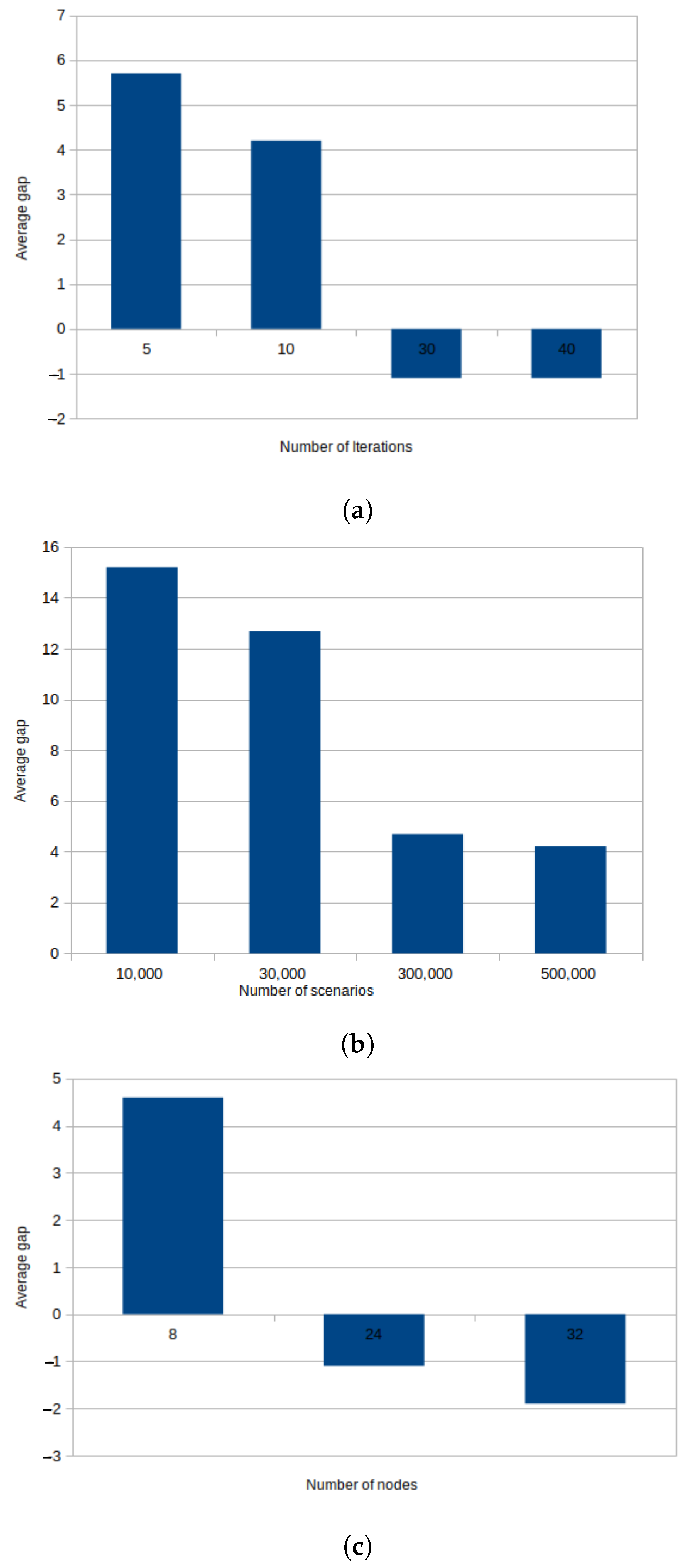
5.5. Sensitivity to Parameters Configuration

In this section, we analyze the effect of changing the number of policy iterations, the number of training scenarios, and the number of the NN hidden layer nodes on the solution quality presented as the percentage average gap between the total cost output of the simulation running the $\mathrm{D}\mathrm{R}\mathrm{L}\mathrm{V}1$ first-stage solution provided with new parameters, as compared to $\mathrm{D}\mathrm{R}\mathrm{L}\mathrm{V}1$ first-stage solution run with default parameters. We change each of the parameters independently while maintaining the other parameters as default. This is reported in Figure 4a–c, respectively.

In Figure 4a,b, we note that decreasing the number of training scenarios can be compensated by increasing the number of policy iterations to maintain solution quality and vice versa. It would be a matter of identifying which combination of both provides the best time performance. Since the policy evaluation phase of our algorithm is very fast, due to the simple recourse, we have opted to increase the number of training scenarios as default.

In Figure 4c, we analyze the effects of increasing NN size on the solution quality. We experience the same effect as with the other experiments. Overall, the number of nodes is a determinant of the solution quality.

5.6. Algorithms Performance

In

Table 5. Time performance in seconds.

$\left|\mathbf{C}\right|$	$\mathbf{DRLV}1$	$\mathbf{DRlV}2$
10	1969.44	2064.23
30	8630.00	8047.11
70	25,114.83	23,515.00
150	64,470.00	62,458.00
300	144,233.00	141,087.00

, we present the time performance of algorithms $\mathrm{D}\mathrm{R}\mathrm{L}\mathrm{V}1$ and $\mathrm{D}\mathrm{R}\mathrm{L}\mathrm{V}2$. It reports the average total time to find offline the first-stage solution, by the number of customers $\left|\mathrm{C}\right|$. We note that the time spent by both algorithms can be further altered by adjusting the solution quality through parameters number of policy iterations, number of training episodes, and number of NN nodes.

Both $\mathrm{D}\mathrm{R}\mathrm{L}\mathrm{V}1$ and $\mathrm{D}\mathrm{R}\mathrm{L}\mathrm{V}2$ scale well for the number of customers and can be used to solve large instances. Since both algorithms run offline, they can be used for dynamic routing decisions when the scenarios are revealed. If time performance is not a critical issue, $\mathrm{D}\mathrm{R}\mathrm{L}\mathrm{V}1$ should be preferred since it provides better quality solutions.

6. Conclusions

In this work, we study an alternative solution approach for a stochastic and dynamic crowdshipping last-mile delivery problem with endogenous uncertainty and solve it approximately using a DRL method. In our approach, it is possible to capture uncertainty related to customers’ online orders and occasional drivers’ availability. The integration of machine learning and operations research optimization techniques have worked as an appropriate alternative to handle the large state and action space.

Computational results demonstrate that the method is capable of making appropriate decisions throughout the day resulting in optimized solutions that reduce total costs when compared to benchmark algorithms implemented. Most importantly, we were able to show the advantages of implementing an alternative to flexible compensation fees, leveraging the power of generative methods to create scenarios and contributing to the advance of knowledge in this topic of the literature.

We foresee directions for future research. The challenge of solving larger instances can motivate the future development of algorithmic methods using a more sophisticated DRL approach, for instance. Many steps of the algorithms can be performed in parallel mode. Action-value learning algorithms, instead of a value-based function approximation approach as we have implemented can be studied. Moreover, different neural network architectures that better capture the sequence dependence nature of the problem can be used to better approximate the DRL method value function. Additionally, in this work we study a flexible compensation scheme, but that is not dynamic. A dynamic compensation scheme would define compensation schemes as a new decision at each stage (decision point). From a business point of view, it would be useful to integrate dynamic decisions with the possibility of online learning, where the data is also offered dynamically. Reinforcement learning methods are natural candidates for online learning, and the challenges associated with this new approach could be studied as an extension of this work.

References

1. ARC Advisory Group. What Are Omni-Channel Fulfillment and Returns Management All about? 2021. Available online: https://www.arcweb.com/industry-best-practices/what-omni-channel-fulfillment-returns-management-all-about (accessed on 18 October 2021).
2. Walmart. Spark Driver Delivery. 2021. Available online: https://drive4spark.walmart.com/ (accessed on 18 October 2021).
3. Doordash. Delivering with Doordash. 2021. Available online: https://www.doordash.com/about/ (accessed on 18 October 2021).
4. JD-Dada. Become a Dada Knight. 2021. Available online: https://www.imdada.cn/ (accessed on 18 October 2021).
5. Archetti, C.; Savelsbergh, M.W.P.; Speranza, M.G. The Vehicle Routing Problem with Occasional Drivers. Eur. J. Oper. Res. 2016, 254, 472–480. [Google Scholar] [CrossRef]
6. Gdowska, K.; Viana, A.; Pedroso, J.P. Stochastic last-mile delivery with crowdshipping. Transp. Res. Procedia 2018, 30, 90–100. [Google Scholar] [CrossRef]
7. Dahle, L.; Andersson, H.; Christiansen, M. The Vehicle Routing Problem with Dynamic Occasional Drivers. In Proceedings of the Computational Logistics; Bektaş, T., Coniglio, S., Martinez-Sykora, A., Voß, S., Eds.; Springer International Publishing: Cham, Switzerland, 2017; pp. 49–63. [Google Scholar]
8. Dayarian, I.; Savelsbergh, M. Crowdshipping and Same-day Delivery: Employing In-store Customers to Deliver Online Orders. Prod. Oper. Manag. 2020, 29, 2153–2174. [Google Scholar] [CrossRef]
9. Arslan, A.M.; Agatz, N.; Kroon, L.; Zuidwijk, R. Crowdsourced Delivery—A Dynamic Pickup and Delivery Problem with Ad Hoc Drivers. Transp. Sci. 2019, 53, 222–235. [Google Scholar] [CrossRef] [Green Version]
10. Barbosa, M. A Data-Driven Compensation Scheme for Last-Mile Delivery with Crowdsourcing. Master’s Thesis, Universidade do Porto, Porto, Portugal, 2019. Available online: https://repositorio-aberto.up.pt/bitstream/10216/124212/2/367287.pdf (accessed on 20 September 2022).
11. Silva, M.; Pedroso, J.P.; Viana, A. Deep Reinforcement Learning for Stochastic Last-Mile Delivery with Crowd Shipping. Available online: https://hal.archives-ouvertes.fr/view/index/docid/3821656 (accessed on 20 September 2022).
12. Dahle, L.; Andersson, H.; Christiansen, M.; Speranza, M.G. The pickup and delivery problem with time windows and occasional drivers. Comput. Oper. Res. 2019, 109, 122–133. [Google Scholar] [CrossRef]
13. Alnaggar, A.; Gzara, F.; Bookbinder, J.H. Crowdsourced delivery: A review of platforms and academic literature. Omega 2019, 98, 102139. [Google Scholar] [CrossRef]
14. Jaillet, P. A Priori Solution of a Traveling Salesman Problem in Which a Random Subset of the Customers Are Visited. Oper. Res. 1988, 36, 929–936. [Google Scholar] [CrossRef] [Green Version]
15. Bertsimas, D.J. A Vehicle Routing Problem with Stochastic Demand. Oper. Res. 1992, 40, 574–585. [Google Scholar] [CrossRef]
16. Laporte, G.; Louveaux, F.V.; Mercure, H. A Priori Optimization of the Probabilistic Traveling Salesman Problem. Oper. Res. 1994, 42, 543–549. [Google Scholar] [CrossRef]
17. Gendreau, M.; Laporte, G.; Séguin, R. An Exact Algorithm for the Vehicle Routing Problem with Stochastic Demands and Customers. Transp. Sci. 1995, 29, 143–155. [Google Scholar] [CrossRef]
18. Laporte, G.; Louveaux, F.V.; van Hamme, L. An Integer L-Shaped Algorithm for the Capacitated Vehicle Routing Problem with Stochastic Demands. Oper. Res. 2002, 50, 415–423. [Google Scholar] [CrossRef] [Green Version]
19. Gauvin, C.; Desaulniers, G.; Gendreau, M. A branch-cut-and-price algorithm for the vehicle routing problem with stochastic demands. Comput. Oper. Res. 2014, 50, 141–153. [Google Scholar] [CrossRef]
20. Amar, M.A.; Khaznaji, W.; Bellalouna, M. An Exact Resolution for the Probabilistic Traveling Salesman Problem under the A Priori Strategy. Procedia Comput. Sci. 2017, 108, 1414–1423. [Google Scholar] [CrossRef]
21. Vaidya, J.; Li, J. A Parallel Branch and Bound Algorithm for the Probabilistic TSP. In Algorithms and Architectures for Parallel Processing, Proceedings of the 18th International Conference, ICA3PP 2018, Guangzhou, China, 15–17 November 2018; Vaidya, J.; Li, J. Springer International Publishing: Cham, Switzerland, 2018; pp. 437–448. [Google Scholar]
22. Lagos, F.; Klapp, M.; Toriello, A. Branch-and-Price for Probabilistic Vehicle Routing. 2017. Available online: http://www.optimization-online.org/DB_HTML/2017/12/6364.html (accessed on 20 September 2022).
23. Novoa, C.; Berger, R.; Linderoth, J.; Storer, R. A Set-Partitioning-Based Model for the Stochastic Vehicle Routing Problem. 2007. Available online: http://www.optimization-online.org/DB_HTML/2006/12/1542.html (accessed on 20 September 2022).
24. Chen, X.; Sim, M.; Sun, P. A Robust Optimization Perspective on Stochastic Programming. Oper. Res. 2007, 55, 1058–1071. [Google Scholar] [CrossRef] [Green Version]
25. Goh, J.; Sim, M. Distributionally Robust Optimization and Its Tractable Approximations. Oper. Res. 2010, 58, 902–917. [Google Scholar] [CrossRef]
26. Delage, E.; Ye, Y. Distributionally Robust Optimization Under Moment Uncertainty with Application to Data-Driven Problems. Oper. Res. 2010, 58, 595–612. [Google Scholar] [CrossRef] [Green Version]
27. Dinh, T.; Fukasawa, R.; Luedtke, J. Exact algorithms for the chance-constrained vehicle routing problem. Math. Program. 2018, 172, 105–138. [Google Scholar] [CrossRef]
28. Ghosal, S.K.; Wiesemann, W. The Distributionally Robust Chance Constrained Vehicle Routing Problem. 2018. Available online: http://www.optimization-online.org/DB_FILE/2018/08/6759.pdf (accessed on 20 September 2022).
29. Bello, I.; Pham, H.; Le, Q.V.; Norouzi, M.; Bengio, S. Neural Combinatorial Optimization with Reinforcement Learning. arXiv 2016, arXiv:1611.09940. [Google Scholar]
30. Nazari, M.; Oroojlooy, A.; Snyder, L.V.; Takác, M. Reinforcement Learning for Solving the Vehicle Routing Problem. In Proceedings of the Advances in Neural Information Processing Systems 31: Annual Conference on Neural Information Processing Systems 2018, NeurIPS 2018, Montréal, QC, Canada, 3–8 December 2018, Montréal, QC, Canada, 3–8 December 2018; Bengio, S., Wallach, H.M., Larochelle, H., Grauman, K., Cesa-Bianchi, N., Garnett, R., Eds.; Curran Associates: New York, NY, USA, 2018; pp. 9861–9871. [Google Scholar]
31. Delarue, A.; Anderson, R.; Tjandraatmadja, C. Reinforcement Learning with Combinatorial Actions: An Application to Vehicle Routing. In Proceedings of the Advances in Neural Information Processing Systems 33: Annual Conference on Neural Information Processing Systems 2020, NeurIPS 2020, Virtual, 6–12 December 2020; Larochelle, H., Ranzato, M., Hadsell, R., Balcan, M., Lin, H., Eds.; 2020. [Google Scholar]
32. Anderson, R.; Huchette, J.; Ma, W.; Tjandraatmadja, C.; Vielma, J.P. Strong mixed-integer programming formulations for trained neural networks. Math. Program. 2020, 183, 3–39. [Google Scholar] [CrossRef] [Green Version]
33. Chen, Y.; Qian, Y.; Yao, Y.; Wu, Z.; Li, R.; Zhou, Y.; Hu, H.; Xu, Y. Can Sophisticated Dispatching Strategy Acquired by Reinforcement Learning?—A Case Study in Dynamic Courier Dispatching System. arXiv 2019, arXiv:cs.AI/1903.02716. [Google Scholar]
34. Chen, X.; Ulmer, M.W.; Thomas, B.W. Deep Q-Learning for Same-Day Delivery with a Heterogeneous Fleet of Vehicles and Drones. arXiv 2019, arXiv:1910.11901. [Google Scholar]
35. Hildebrandt, F.D.; Thomas, B.W.; Ulmer, M.W. Where the Action is: Let’s make Reinforcement Learning for Stochastic Dynamic Vehicle Routing Problems work! arXiv 2021, arXiv:2103.00507. [Google Scholar]
36. Pflug, G.C. On-Line Optimization of Simulated Markovian Processes. Math. Oper. Res. 1990, 15, 381–395. [Google Scholar] [CrossRef]
37. Jonsbraten, T.W.; Wets, R.J.B.; Woodruff, D.L. A Class of Stochastic Programs with Decision Dependent Random Elements. Ann. Oper. Res. 1998, 82, 83–106. [Google Scholar] [CrossRef]
38. Goel, V.; Grossmann, I.E. A stochastic programming approach to planning of offshore gas field developments under uncertainty in reserves. Comput. Chem. Eng. 2004, 28, 1409–1429. [Google Scholar] [CrossRef]
39. Goel, V.; Grossmann, I. A Class of stochastic programs with decision dependent uncertainty. Math. Program. 2006, 108, 355–394. [Google Scholar] [CrossRef] [Green Version]
40. Luo, F.; Mehrotra, S. Distributionally Robust Optimization with Decision Dependent Ambiguity Sets. arXiv 2018, arXiv:1806.09215. [Google Scholar] [CrossRef]
41. Balashov, M.; Kiselev, A.; Kuryleva, A. Reinforcement Learning Approach for Dynamic Pricing. In The Economics of Digital Transformation: Approaching Non-Stable and Uncertain Digitalized Production Systems; Devezas, T., Leitão, J., Sarygulov, A., Eds.; Springer International Publishing: Cham, Switzerland, 2021; pp. 123–141. [Google Scholar] [CrossRef]
42. Liu, J.; Zhang, Y.; Wang, X.; Deng, Y.; Wu, X. Dynamic Pricing on E-commerce Platform with Deep Reinforcement Learning: A Field Experiment. arXiv 2019, arXiv:1912.02572. [Google Scholar]
43. Shorten, C.; Khoshgoftaar, T.M. A survey on Image Data Augmentation for Deep Learning. J. Big Data 2019, 6, 60. [Google Scholar] [CrossRef]
44. Koochali, A.; Dengel, A.; Ahmed, S. If You Like It, GAN It—Probabilistic Multivariate Times Series Forecast with GAN. Eng. Proc. 2021, 5, 40. [Google Scholar]
45. Gneiting, T.; Katzfuss, M. Probabilistic Forecasting. Annu. Rev. Stat. Its Appl. 2014, 1, 125–151. [Google Scholar] [CrossRef]
46. Goodfellow, I.; Pouget-Abadie, J.; Mirza, M.; Xu, B.; Warde-Farley, D.; Ozair, S.; Courville, A.; Bengio, Y. Generative Adversarial Networks. Adv. Neural Inf. Process. Syst. 2014, 3, 2672–2680. [Google Scholar] [CrossRef]
47. Mirza, M.; Osindero, S. Conditional Generative Adversarial Nets. arXiv 2014, arXiv:1411.1784. [Google Scholar]
48. Smith, K.E.; Smith, A.O. Conditional GAN for timeseries generation. arXiv 2020, arXiv:2006.16477. [Google Scholar]
49. Hochreiter, S.; Schmidhuber, J. Long Short-term Memory. Neural Comput. 1997, 9, 1735–17380. [Google Scholar] [CrossRef]
50. Weiler, C.; Biesinger, B.; Hu, B.; Raidl, G.R. Heuristic Approaches for the Probabilistic Traveling Salesman Problem. In Computer Aided Systems Theory—EUROCAST 2015, Proceedings of the 15th International Conference, Las Palmas de Gran Canaria, Spain, 8–13 February 2015; Moreno-Díaz, R., Pichler, F., Quesada-Arencibia, A., Eds.; Springer International Publishing: Cham, Switzerland, 2015; pp. 342–349. [Google Scholar]
Figure 1. Fully connected neural network with one hidden layer and linear output.
Mathematics 10 03902 g001
Figure 2. Conditional GAN.
Mathematics 10 03902 g002
Figure 3. Initial Insights: (a) Instance a and optimal 2 routes; (b) Instance b and optimal 2 routes; (c) Instance c and optimal 3 routes; (d) Instance a and optimal 3 routes.
Mathematics 10 03902 g003
Figure 4. Sensitivity to key parameters: (a) Effect of number of policy iterations; (b) Effect of number of training scenarios; (c) Effect of number of NN hidden layer nodes.
Mathematics 10 03902 g004