
Survey on Synthetic Data Generation, Evaluation Methods and GANs


Abstract
:1. Introduction
2. Literature Review
| Listing 1. Query used to search the WoS, Scopus, IEEE, and ACM databases. |
 |
3. Generative Adversarial Networks
3.1. GANs under the Hood
3.2. Main Drawbacks
3.3. GANs Come in a Lot of Flavours
3.4. GANs for Tabular Data
3.4.1. TGAN
3.4.2. CTGAN
3.4.3. TabFairGAN
4. Methods for the Generation of Synthetic Samples
4.1. Standard Methods
4.1.1. Random Oversampling (ROS)
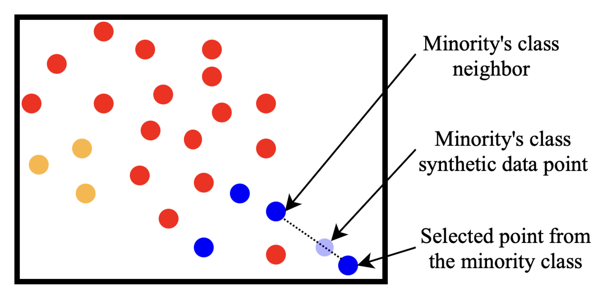
4.1.2. Synthetic Minority Oversampling Technique (SMOTE)
4.1.3. Borderline-SMOTE
4.1.4. Safe-Level-SMOTE
4.1.5. ADASYN
4.1.6. K-Means SMOTE
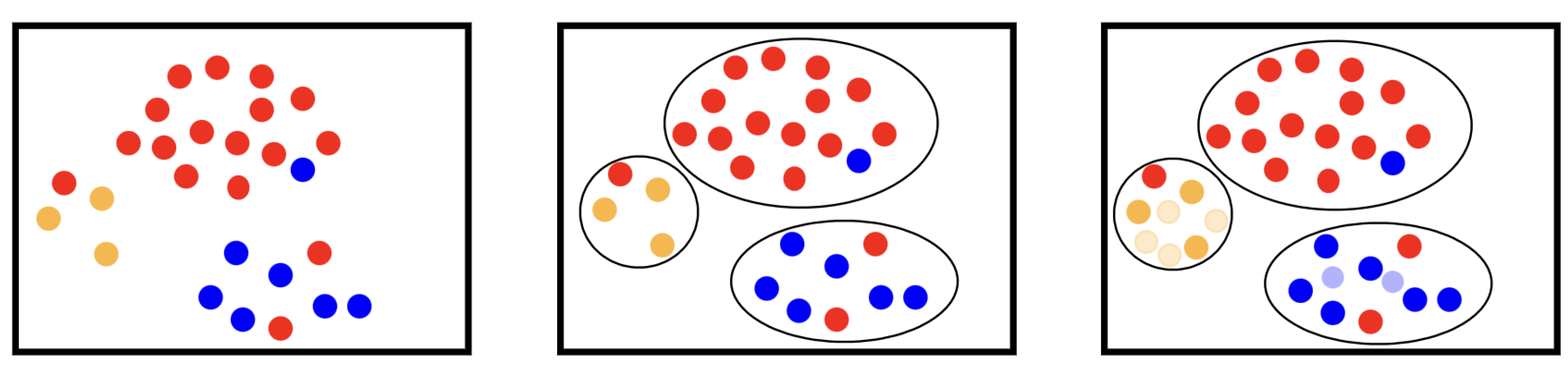
4.1.7. Cluster-Based Oversampling
4.1.8. Gaussian Mixture Model
4.2. Deep Learning Methods
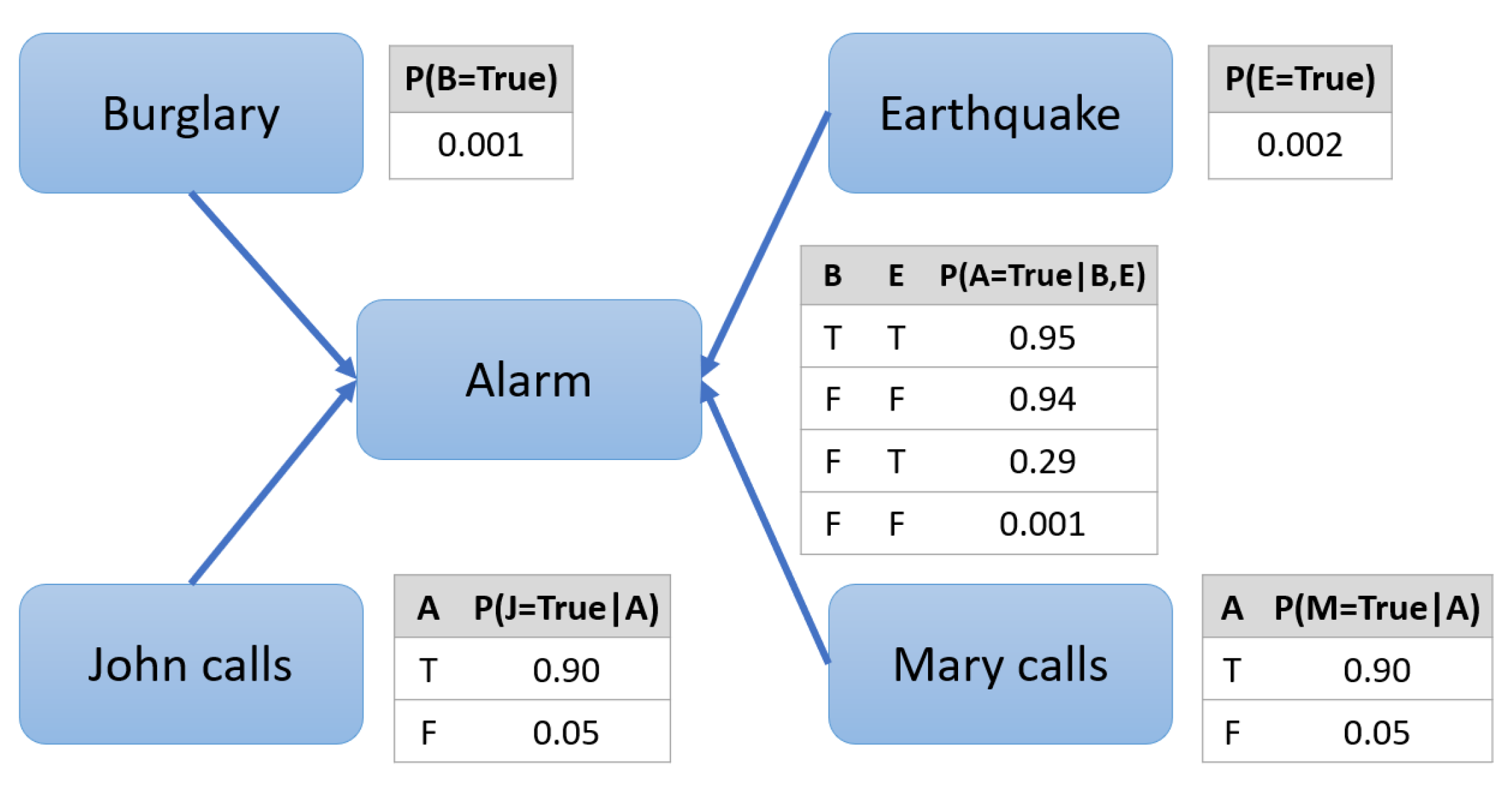
4.2.1. Bayesian Networks
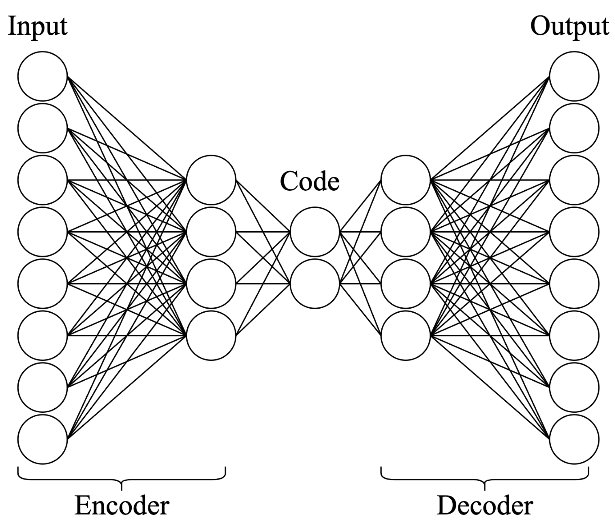
4.2.2. Autoencoders
4.2.3. Generative Adversarial Networks
4.3. Thoughts on the Algorithms
5. Synthetic Sample Quality Evaluation
6. Discussion
7. Conclusions
Author Contributions
Funding
Institutional Review Board Statement
Informed Consent Statement
Data Availability Statement
Acknowledgments
Conflicts of Interest
References
- Emam, K.; Mosquera, L.; Hoptroff, R. Chapter 1: Introducing Synthetic Data Generation. In Practical Synthetic Data Generation: Balancing Privacy and the Broad Availability of Data; O’Reilly Media, Inc.: Sebastopol, CA, USA, 2020; pp. 1–22. [Google Scholar]
- Chawla, N.V.; Bowyer, K.W.; Hall, L.O.; Kegelmeyer, W.P. SMOTE: Synthetic minority over-sampling technique. J. Artif. Intell. Res. 2002, 16, 321–357. [Google Scholar] [CrossRef]
- Han, H.; Wang, W.Y.; Mao, B.H. Borderline-SMOTE: A new over-sampling method in imbalanced data sets learning. In Proceedings of the International Conference on Intelligent Computing, Hefei, China, 23–26 August 2005; pp. 878–887. [Google Scholar]
- Bunkhumpornpat, C.; Sinapiromsaran, K.; Lursinsap, C. Safe-level-smote: Safe-level-synthetic minority over-sampling technique for handling the class imbalanced problem. In Proceedings of the Pacific-Asia Conference on Knowledge Discovery and Data Mining, Bangkok, Thailand, 27–30 April 2009; pp. 475–482. [Google Scholar]
- He, H.; Bai, Y.; Garcia, E.A.; Li, S. ADASYN: Adaptive synthetic sampling approach for imbalanced learning. In Proceedings of the 2008 IEEE International Joint Conference on Neural Networks (IEEE World Congress on Computational Intelligence), Hong Kong, China, 1–8 June 2008; pp. 1322–1328. [Google Scholar]
- Douzas, G.; Bacao, F.; Last, F. Improving imbalanced learning through a heuristic oversampling method based on k-means and SMOTE. Inf. Sci. 2018, 465, 1–20. [Google Scholar] [CrossRef] [Green Version]
- Kingma, D.P.; Welling, M. Auto-encoding variational bayes. arXiv 2013, arXiv:1312.6114. [Google Scholar]
- Goodfellow, I.; Pouget-Abadie, J.; Mirza, M.; Xu, B.; Warde-Farley, D.; Ozair, S.; Courville, A.; Bengio, Y. Generative adversarial nets. In Proceedings of the Advances in Neural Information Processing Systems 27 (NIPS 2014), Montreal, QC, Canada, 8–13 December 2014; Volume 27. [Google Scholar]
- Siddani, B.; Balachandar, S.; Moore, W.C.; Yang, Y.; Fang, R. Machine learning for physics-informed generation of dispersed multiphase flow using generative adversarial networks. Theor. Comput. Fluid Dyn. 2021, 35, 807–830. [Google Scholar] [CrossRef]
- Coutinho-Almeida, J.; Rodrigues, P.P.; Cruz-Correia, R.J. GANs for Tabular Healthcare Data Generation: A Review on Utility and Privacy. In Discovery Science; Soares, C., Torgo, L., Eds.; Springer International Publishing: Cham, Switzerland, 2021; pp. 282–291. [Google Scholar]
- Gupta, A.; Vedaldi, A.; Zisserman, A. Synthetic data for text localisation in natural images. In Proceedings of the IEEE Conference on Computer Vision and Pattern Recognition, Las Vegas, NV, USA, 26 June–1 July 2016; pp. 2315–2324. [Google Scholar]
- Bolón-Canedo, V.; Sánchez-Maroño, N.; Alonso-Betanzos, A. A review of feature selection methods on synthetic data. Knowl. Inf. Syst. 2013, 34, 483–519. [Google Scholar] [CrossRef]
- Frid-Adar, M.; Klang, E.; Amitai, M.; Goldberger, J.; Greenspan, H. Synthetic data augmentation using GAN for improved liver lesion classification. In Proceedings of the 2018 IEEE 15th International Symposium on Biomedical Imaging (ISBI 2018), Washington, DC, USA, 4–7 April 2018; pp. 289–293. [Google Scholar]
- Koch, B. Status and future of laser scanning, synthetic aperture radar and hyperspectral remote sensing data for forest biomass assessment. ISPRS J. Photogramm. Remote Sens. 2010, 65, 581–590. [Google Scholar] [CrossRef]
- Wu, X.; Liang, L.; Shi, Y.; Fomel, S. FaultSeg3D: Using synthetic data sets to train an end-to-end convolutional neural network for 3D seismic fault segmentation. Geophysics 2019, 84, IM35–IM45. [Google Scholar] [CrossRef]
- Nikolenko, S.I. Synthetic Data Outside Computer Vision. In Synthetic Data for Deep Learning; Springer: Berlin/Heidelberg, Germany, 2021; pp. 217–226. [Google Scholar]
- Pan, Z.; Yu, W.; Yi, X.; Khan, A.; Yuan, F.; Zheng, Y. Recent progress on generative adversarial networks (GANs): A survey. IEEE Access 2019, 7, 36322–36333. [Google Scholar] [CrossRef]
- Di Mattia, F.; Galeone, P.; De Simoni, M.; Ghelfi, E. A survey on gans for anomaly detection. arXiv 2019, arXiv:1906.11632. [Google Scholar]
- Saxena, D.; Cao, J. Generative adversarial networks (GANs) challenges, solutions, and future directions. ACM Comput. Surv. (CSUR) 2021, 54, 1–42. [Google Scholar] [CrossRef]
- Wang, Q.; Gao, J.; Lin, W.; Yuan, Y. Learning from synthetic data for crowd counting in the wild. In Proceedings of the IEEE/CVF Conference on Computer Vision and Pattern Recognition, Long Beach, CA, USA, 16–17 June 2019; pp. 8198–8207. [Google Scholar]
- Atapour-Abarghouei, A.; Breckon, T.P. Real-time monocular depth estimation using synthetic data with domain adaptation via image style transfer. In Proceedings of the IEEE Conference on Computer Vision and Pattern Recognition, Salt Lake City, UT, USA, 18–23 June 2018; pp. 2800–2810. [Google Scholar]
- Liu, J.; Qu, F.; Hong, X.; Zhang, H. A small-sample wind turbine fault detection method with synthetic fault data using generative adversarial nets. IEEE Trans. Ind. Inform. 2018, 15, 3877–3888. [Google Scholar] [CrossRef]
- Zhang, L.; Gonzalez-Garcia, A.; Van De Weijer, J.; Danelljan, M.; Khan, F.S. Synthetic data generation for end-to-end thermal infrared tracking. IEEE Trans. Image Process. 2018, 28, 1837–1850. [Google Scholar] [CrossRef] [PubMed] [Green Version]
- Wang, Q.; Gao, J.; Lin, W.; Yuan, Y. Pixel-wise crowd understanding via synthetic data. Int. J. Comput. Vis. 2021, 129, 225–245. [Google Scholar] [CrossRef]
- Chen, Y.; Li, W.; Chen, X.; Gool, L.V. Learning semantic segmentation from synthetic data: A geometrically guided input-output adaptation approach. In Proceedings of the IEEE/CVF Conference on Computer Vision and Pattern Recognition, Long Beach, CA, USA, 15–20 June 2019; pp. 1841–1850. [Google Scholar]
- Dunn, K.W.; Fu, C.; Ho, D.J.; Lee, S.; Han, S.; Salama, P.; Delp, E.J. DeepSynth: Three-dimensional nuclear segmentation of biological images using neural networks trained with synthetic data. Sci. Rep. 2019, 9, 18295. [Google Scholar] [CrossRef] [PubMed] [Green Version]
- Kim, K.; Myung, H. Autoencoder-combined generative adversarial networks for synthetic image data generation and detection of jellyfish swarm. IEEE Access 2018, 6, 54207–54214. [Google Scholar] [CrossRef]
- Torkzadehmahani, R.; Kairouz, P.; Paten, B. Dp-cgan: Differentially private synthetic data and label generation. In Proceedings of the IEEE/CVF Conference on Computer Vision and Pattern Recognition Workshops, Long Beach, CA, USA, 16–17 June 2019. [Google Scholar]
- Mirza, M.; Osindero, S. Conditional generative adversarial nets. arXiv 2014, arXiv:1411.1784. [Google Scholar]
- Radford, A.; Metz, L.; Chintala, S. Unsupervised representation learning with deep convolutional generative adversarial networks. arXiv 2015, arXiv:1511.06434. [Google Scholar]
- Chen, X.; Duan, Y.; Houthooft, R.; Schulman, J.; Sutskever, I.; Abbeel, P. Infogan: Interpretable representation learning by information maximizing generative adversarial nets. In Proceedings of the 30th International Conference on Neural Information Processing Systems, Barcelona, Spain, 5–10 December 2016; pp. 2180–2188. [Google Scholar]
- Liu, M.Y.; Tuzel, O. Coupled generative adversarial networks. Adv. Neural Inf. Process. Syst. 2016, 29, 469–477. [Google Scholar]
- Odena, A.; Olah, C.; Shlens, J. Conditional image synthesis with auxiliary classifier gans. In Proceedings of the International Conference on Machine Learning, PMLR, Sydney, Australia, 6–11 August 2017; pp. 2642–2651. [Google Scholar]
- Zhang, H.; Xu, T.; Li, H.; Zhang, S.; Wang, X.; Huang, X.; Metaxas, D.N. Stackgan: Text to photo-realistic image synthesis with stacked generative adversarial networks. In Proceedings of the IEEE International Conference on Computer Vision, Venice, Italy, 22–29 October 2017; pp. 5907–5915. [Google Scholar]
- Arjovsky, M.; Chintala, S.; Bottou, L. Wasserstein generative adversarial networks. In Proceedings of the International Conference on Machine Learning, PMLR, Sydney, Australia, 6–11 August 2017; pp. 214–223. [Google Scholar]
- Zhu, J.Y.; Park, T.; Isola, P.; Efros, A.A. Unpaired image-to-image translation using cycle-consistent adversarial networks. In Proceedings of the IEEE International Conference on Computer Vision, Venice, Italy, 22–29 October 2017; pp. 2223–2232. [Google Scholar]
- Dong, H.W.; Hsiao, W.Y.; Yang, L.C.; Yang, Y.H. MuseGAN: Multi-track Sequential Generative Adversarial Networks for Symbolic Music Generation and Accompaniment. arXiv 2017, arXiv:1709.06298. [Google Scholar] [CrossRef]
- Karras, T.; Aila, T.; Laine, S.; Lehtinen, J. Progressive growing of gans for improved quality, stability, and variation. arXiv 2017, arXiv:1710.10196. [Google Scholar]
- Zhang, H.; Goodfellow, I.; Metaxas, D.; Odena, A. Self-attention generative adversarial networks. In Proceedings of the International Conference on Machine Learning, PMLR, Long Beach, CA, USA, 9–15 June 2019; pp. 7354–7363. [Google Scholar]
- Salimans, T.; Goodfellow, I.; Zaremba, W.; Cheung, V.; Radford, A.; Chen, X. Improved Techniques for Training GANs. arXiv 2016, arXiv:1606.03498. [Google Scholar]
- Heusel, M.; Ramsauer, H.; Unterthiner, T.; Nessler, B.; Hochreiter, S. GANs Trained by a Two Time-Scale Update Rule Converge to a Local Nash Equilibrium. arXiv 2018, arXiv:1706.08500. [Google Scholar]
- Brock, A.; Donahue, J.; Simonyan, K. Large scale GAN training for high fidelity natural image synthesis. arXiv 2018, arXiv:1809.11096. [Google Scholar]
- Karras, T.; Laine, S.; Aila, T. A style-based generator architecture for generative adversarial networks. In Proceedings of the IEEE/CVF Conference on Computer Vision and Pattern Recognition, Long Beach, CA, USA, 15–20 June 2019; pp. 4401–4410. [Google Scholar]
- Park, T.; Liu, M.Y.; Wang, T.C.; Zhu, J.Y. Semantic image synthesis with spatially-adaptive normalization. In Proceedings of the IEEE/CVF Conference on Computer Vision and Pattern Recognition, Long Beach, CA, USA, 15–20 June 2019; pp. 2337–2346. [Google Scholar]
- Cai, W.; Wei, Z. PiiGAN: Generative adversarial networks for pluralistic image inpainting. IEEE Access 2020, 8, 48451–48463. [Google Scholar] [CrossRef]
- Prangemeier, T.; Reich, C.; Wildner, C.; Koeppl, H. Multi-StyleGAN: Towards Image-Based Simulation of Time-Lapse Live-Cell Microscopy. arXiv 2021, arXiv:2106.08285. [Google Scholar]
- Xu, L.; Veeramachaneni, K. Synthesizing tabular data using generative adversarial networks. arXiv 2018, arXiv:1811.11264. [Google Scholar]
- Xu, L.; Skoularidou, M.; Cuesta-Infante, A.; Veeramachaneni, K. Modeling tabular data using conditional gan. arXiv 2019, arXiv:1907.00503. [Google Scholar]
- Chow, C.; Liu, C. Approximating discrete probability distributions with dependence trees. IEEE Trans. Inf. Theory 1968, 14, 462–467. [Google Scholar] [CrossRef] [Green Version]
- Zhang, J.; Cormode, G.; Procopiuc, C.M.; Srivastava, D.; Xiao, X. Privbayes: Private data release via bayesian networks. ACM Trans. Database Syst. (TODS) 2017, 42, 1–41. [Google Scholar] [CrossRef]
- Choi, E.; Biswal, S.; Malin, B.; Duke, J.; Stewart, W.F.; Sun, J. Generating multi-label discrete patient records using generative adversarial networks. In Proceedings of the Machine Learning for Healthcare Conference, PMLR, Boston, MA, USA, 18–19 August 2017; pp. 286–305. [Google Scholar]
- Srivastava, A.; Valkov, L.; Russell, C.; Gutmann, M.U.; Sutton, C. Veegan: Reducing mode collapse in gans using implicit variational learning. In Proceedings of the Advances in Neural Information Processing Systems 30 (NIPS 2017), Long Beach, CA, USA, 4–9 December 2017; Volume 30. [Google Scholar]
- Park, N.; Mohammadi, M.; Gorde, K.; Jajodia, S.; Park, H.; Kim, Y. Data synthesis based on generative adversarial networks. arXiv 2018, arXiv:1806.03384. [Google Scholar] [CrossRef] [Green Version]
- Rajabi, A.; Garibay, O.O. TabFairGAN: Fair Tabular Data Generation with Generative Adversarial Networks. arXiv 2021, arXiv:2109.00666. [Google Scholar] [CrossRef]
- Andrews, G. What Is Synthetic Data? 2021. Available online: https://blogs.nvidia.com/blog/2021/06/08/what-is-synthetic-data/ (accessed on 14 February 2022).
- Alanazi, Y.; Sato, N.; Ambrozewicz, P.; Blin, A.N.H.; Melnitchouk, W.; Battaglieri, M.; Liu, T.; Li, Y. A survey of machine learning-based physics event generation. arXiv 2021, arXiv:2106.00643. [Google Scholar]
- Assefa, S. Generating synthetic data in finance: Opportunities, challenges and pitfalls. In Proceedings of the International Conference on AI in Finance, New York, NY, USA, 15–16 October 2020. [Google Scholar]
- Lan, L.; You, L.; Zhang, Z.; Fan, Z.; Zhao, W.; Zeng, N.; Chen, Y.; Zhou, X. Generative Adversarial Networks and Its Applications in Biomedical Informatics. Front. Public Health 2020, 8, 164. [Google Scholar] [CrossRef] [PubMed]
- Chen, J.; Little, J.J. Sports camera calibration via synthetic data. In Proceedings of the IEEE/CVF Conference on Computer Vision and Pattern Recognition Workshops, Long Beach, CA, USA, 16–20 June 2019. [Google Scholar]
- Barth, R.; IJsselmuiden, J.; Hemming, J.; van Henten, E.J. Optimising realism of synthetic agricultural images using cycle generative adversarial networks. In Proceedings of the IEEE IROS Workshop on Agricultural Robotics, Vancouver, BC, Canada, 28 September 2017; pp. 18–22. [Google Scholar]
- Tremblay, J.; To, T.; Sundaralingam, B.; Xiang, Y.; Fox, D.; Birchfield, S. Deep object pose estimation for semantic robotic grasping of household objects. arXiv 2018, arXiv:1809.10790. [Google Scholar]
- Nikolenko, S.I. Synthetic data for deep learning. arXiv 2019, arXiv:1909.11512. [Google Scholar]
- Batuwita, R.; Palade, V. Efficient resampling methods for training support vector machines with imbalanced datasets. In Proceedings of the 2010 International Joint Conference on Neural Networks (IJCNN), Barcelona, Spain, 18–23 July 2010; pp. 1–8. [Google Scholar]
- Drummond, C.; Holte, R.C. C4. 5, class imbalance, and cost sensitivity: Why under-sampling beats over-sampling. Workshop Learn. Imbalanced Datasets II 2003, 11, 1–8. [Google Scholar]
- Lusa, L. Evaluation of smote for high-dimensional class-imbalanced microarray data. In Proceedings of the 2012 11th International Conference on Machine Learning and Applications, Boca Raton, FL, USA, 12–15 December 2012; Volume 2, pp. 89–94. [Google Scholar]
- Sun, J.; Lang, J.; Fujita, H.; Li, H. Imbalanced enterprise credit evaluation with DTE-SBD: Decision tree ensemble based on SMOTE and bagging with differentiated sampling rates. Inf. Sci. 2018, 425, 76–91. [Google Scholar] [CrossRef]
- Sun, J.; Li, H.; Fujita, H.; Fu, B.; Ai, W. Class-imbalanced dynamic financial distress prediction based on Adaboost-SVM ensemble combined with SMOTE and time weighting. Inf. Fusion 2020, 54, 128–144. [Google Scholar] [CrossRef]
- Lee, T.; Kim, M.; Kim, S.P. Data augmentation effects using borderline-SMOTE on classification of a P300-based BCI. In Proceedings of the 2020 8th International Winter Conference on Brain-Computer Interface (BCI), Gangwon, Korea, 26–28 February 2020; pp. 1–4. [Google Scholar]
- Riafio, D. Using Gabriel graphs in Borderline-SMOTE to deal with severe two-class imbalance problems on neural networks. In Artificial Intelligence Research and Development, Proceedings of the 15th International Conference of the Catalan Association for Artificial Intelligence, Alicante, Spain, 24–26 October 2012; IOS Press: Amsterdam, The Netherlands, 2012; Volume 248, p. 29. [Google Scholar]
- Siriseriwan, W.; Sinapiromsaran, K. The effective redistribution for imbalance dataset: Relocating safe-level SMOTE with minority outcast handling. Chiang Mai J. Sci. 2016, 43, 234–246. [Google Scholar]
- Lu, C.; Lin, S.; Liu, X.; Shi, H. Telecom fraud identification based on ADASYN and random forest. In Proceedings of the 2020 5th International Conference on Computer and Communication Systems (ICCCS), Guangzhou, China, 21–24 April 2020; pp. 447–452. [Google Scholar]
- Aditsania, A.; Saonard, A.L. Handling imbalanced data in churn prediction using ADASYN and backpropagation algorithm. In Proceedings of the 2017 3rd International Conference on Science in Information Technology (ICSITech), Bandung, Indonesia, 25–26 October 2017; pp. 533–536. [Google Scholar]
- Chen, S. Research on Extreme Financial Risk Early Warning Based on ODR-ADASYN-SVM. In Proceedings of the 2017 International Conference on Humanities Science, Management and Education Technology (HSMET 2017), Taiyuan, China, 25–26 February 2017; pp. 1132–1137. [Google Scholar]
- MacQueen, J. Classification and analysis of multivariate observations. In Proceedings of the 5th Berkeley Symposium on Mathematical Statistics and Probability; University of California Press: Berkeley, CA, USA, 1967; pp. 281–297. [Google Scholar]
- Sarkar, S.; Pramanik, A.; Maiti, J.; Reniers, G. Predicting and analyzing injury severity: A machine learning-based approach using class-imbalanced proactive and reactive data. Saf. Sci. 2020, 125, 104616. [Google Scholar] [CrossRef]
- Jo, T.; Japkowicz, N. Class imbalances versus small disjuncts. ACM Sigkdd Explor. Newsl. 2004, 6, 40–49. [Google Scholar] [CrossRef]
- Learn, S. Gaussian Mixture Models. 2022. Available online: https://scikit-learn.org/stable/modules/mixture.html (accessed on 23 February 2022).
- Chokwitthaya, C.; Zhu, Y.; Mukhopadhyay, S.; Jafari, A. Applying the Gaussian Mixture Model to Generate Large Synthetic Data from a Small Data Set. In Construction Research Congress 2020: Computer Applications; American Society of Civil Engineers: Reston, VA, USA, 2020; pp. 1251–1260. [Google Scholar]
- A Comprehensive Introduction to Bayesian Deep Learning. Available online: https://jorisbaan.nl/2021/03/02/introduction-to-bayesian-deep-learning (accessed on 11 February 2022).
- Soni, D. Introduction to Bayesian Networks. 2019. Available online: https://towardsdatascience.com/introduction-to-bayesian-networks-81031eeed94e (accessed on 29 January 2022).
- Russell, S.J.; Norvig, P.; Chang, M.W. Chapter 13: Probabilistic Reasoning. In Artificial Intelligence: A Modern Approach; Pearson: London, UK, 2022; pp. 430–478. [Google Scholar]
- Goodfellow, I.; Bengio, Y.; Courville, A. Chapter 20: Deep Generative Models. In Depp Learning; MIT Press: Cambridge, MA, USA, 2016; pp. 654–720. [Google Scholar]
- Foster, D. Chapter 3: Variational Autoencoders. In Generative Deep Learning: Teaching Machines to Paint, Write, Compose, and Play; O’Reilly: Sebastopol, CA, USA, 2019; pp. 61–96. [Google Scholar]
- Goodfellow, I.; Bengio, Y.; Courville, A. Chapter 14: Autoencoders. In Depp Learning; MIT Press: Cambridge, MA, USA, 2016; pp. 502–525. [Google Scholar]
- Zhang, X.; Fu, Y.; Zang, A.; Sigal, L.; Agam, G. Learning classifiers from synthetic data using a multichannel autoencoder. arXiv 2015, arXiv:1503.03163. [Google Scholar]
- Wan, Z.; Zhang, Y.; He, H. Variational autoencoder based synthetic data generation for imbalanced learning. In Proceedings of the 2017 IEEE Symposium Series on Computational Intelligence (SSCI), Honolulu, HI, USA, 27 November–1 December 2017; pp. 1–7. [Google Scholar]
- Islam, Z.; Abdel-Aty, M.; Cai, Q.; Yuan, J. Crash data augmentation using variational autoencoder. Accid. Anal. Prev. 2021, 151, 105950. [Google Scholar] [CrossRef] [PubMed]
- Fahimi, F.; Zhang, Z.; Goh, W.B.; Ang, K.K.; Guan, C. Towards EEG generation using GANs for BCI applications. In Proceedings of the 2019 IEEE EMBS International Conference on Biomedical & Health Informatics (BHI), Chicago, IL, USA, 19–22 May 2019; pp. 1–4. [Google Scholar]
- Patel, M.; Wang, X.; Mao, S. Data augmentation with Conditional GAN for automatic modulation classification. In Proceedings of the 2nd ACM Workshop on Wireless Security and Machine Learning, Linz, Austria, 13 July 2020; pp. 31–36. [Google Scholar]
- Ali-Gombe, A.; Elyan, E. MFC-GAN: Class-imbalanced dataset classification using multiple fake class generative adversarial network. Neurocomputing 2019, 361, 212–221. [Google Scholar] [CrossRef]
- Ali-Gombe, A.; Elyan, E.; Savoye, Y.; Jayne, C. Few-shot classifier GAN. In Proceedings of the 2018 International Joint Conference on Neural Networks (IJCNN), Rio de Janeiro, Brazil, 8–13 July 2018; pp. 1–8. [Google Scholar]
- Sushko, V.; Gall, J.; Khoreva, A. One-shot gan: Learning to generate samples from single images and videos. In Proceedings of the IEEE/CVF Conference on Computer Vision and Pattern Recognition, Nashville, TN, USA, 20–25 June 2021; pp. 2596–2600. [Google Scholar]
- Niu, M.Y.; Zlokapa, A.; Broughton, M.; Boixo, S.; Mohseni, M.; Smelyanskyi, V.; Neven, H. Entangling quantum generative adversarial networks. Phys. Rev. Lett. 2022, 128, 220505. [Google Scholar] [CrossRef]
- Zhang, W.; Ma, Y.; Zhu, D.; Dong, L.; Liu, Y. MetroGAN: Simulating Urban Morphology with Generative Adversarial Network. arXiv 2022, arXiv:2207.02590. [Google Scholar]
- Yann LeCun Quora Session Overview. Available online: https://www.kdnuggets.com/2016/08/yann-lecun-quora-session.html (accessed on 2 February 2022).
- Anscombe, F.J. Graphs in statistical analysis. Am. Stat. 1973, 27, 17–21. [Google Scholar]
- Zhou, Y.; Dong, F.; Liu, Y.; Li, Z.; Du, J.; Zhang, L. Forecasting emerging technologies using data augmentation and deep learning. Scientometrics 2020, 123, 1–29. [Google Scholar] [CrossRef] [Green Version]
- Shmelkov, K.; Schmid, C.; Alahari, K. How good is my GAN? In Proceedings of the European Conference on Computer Vision (ECCV), Munich, Germany, 8–14 September 2018; pp. 213–229. [Google Scholar]
- Alaa, A.M.; van Breugel, B.; Saveliev, E.; van der Schaar, M. How Faithful is your Synthetic Data? Sample-level Metrics for Evaluating and Auditing Generative Models. arXiv 2021, arXiv:2102.08921. [Google Scholar]


| Database | No Filters | Field = Title | Date = 1 January 2010 to 31 December 2022 | Language = English |
|---|---|---|---|---|
| WoS | 167,419 | 2460 | 1699 | 1681 |
| Scopus | 1,168,662 | 3625 | 2457 | 2401 |
| IEEE | 44,887 | 731 | 562 | No filter |
| ACM | 31,463 | 65 | 57 | No filter |
| Unique authors | 10,100 |
| Average number of authors per document | 4.37 |
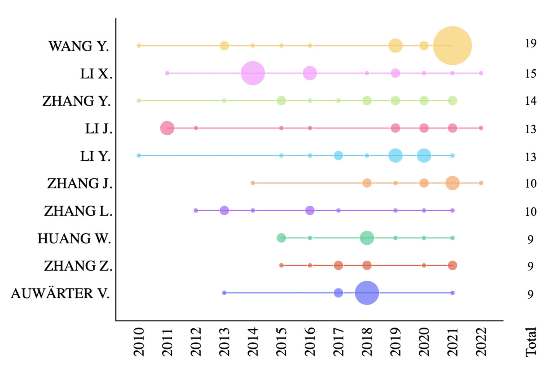
| Most published works | Wang Y. (19 works) Li X. (15 works) |
| Most published works (≥2020) | Wang Y. (6 works) Nikolenko S. I. (4 works) |
| Most cited | Gupta A., Zisserman A., Vedaldi A. (676 citations) Alonso A., Sánchex N., Bolón V. (392 citations) |
| Title | GAN Architecture | Dataset | Year | Citations |
|---|---|---|---|---|
| Synthetic Data Augmentation using GAN for Improved Liver Lesion Classification [13] | DCGAN | Computed tomography (CT) images of 182 liver lesions | 2018 | 173 |
| Learning from Synthetic Data for Crowd Counting in the Wild [20] | SSIM embedding (SE) Cycle GAN | GCC dataset, UCF CC 50, Shanghai Tech A/B, UCF-QNRF, WorldExpo’10 | 2019 | 94 |
| Real-Time Monocular Depth Estimation using Synthetic Data with Domain Adaptation via Image Style Transfer [21] | DCGAN | KITTI, Make3D | 2018 | 53 |
| A Small-Sample Wind Turbine Fault Detection Method with Synthetic Fault Data using Generative Adversarial Nets [22] | CGAN | Wind turbine data collected from a wind farm in northern China | 2019 | 44 |
| Synthetic Data Generation for End-to-End Thermal Infrared Tracking [23] | CycleGAN, Pix2pix | KAIST, CVC-14, OSU Color Thermal, OTB, VAP Trimodal, Bilodeau, LITIV2012, VOT2016, VOT2017, ASL, Long-termInfAR | 2019 | 40 |
| Pixel-Wise Crowd Understanding via Synthetic Data [24] | SE CycleGAN | GCC dataset, UCF CC 50, Shanghai Tech A/B, UCF-QNRF | 2021 | 33 |
| Learning Semantic Segmentation from Synthetic Data: A Geometrically Guided Input-Output Adaptation Approach [25] | PatchGAN | KITTI, Virtual KITTI, SYNTHIA Cityscapes | 2019 | 25 |
| DeepSynth: Three-dimensional Nuclear Segmentation of Biological Images using Neural Networks Trained with Synthetic Data [26] | Spatially Constrained (SP) CycleGAN | 3D biological images | 2019 | 23 |
| Autoencoder-Combined Generative Adversarial Networks for Synthetic Image Data Generation and Detection of Jellyfish Swarm [27] | GAN | Jellyfish images | 2018 | 13 |
| DP-CGAN: Differentially Private Synthetic Data and Label Generation [28] | Differentially Private Conditional GAN (DP-CGAN) | MNIST | 2019 | 10 |
| Methods | Method Type | References |
|---|---|---|
| Random Oversampling (ROS) | Standard | [63,64] |
| SMOTE | Standard | [2,65,66,67] |
| Borderline-SMOTE | Standard | [3,68,69] |
| Safe-Level-SMOTE | Standard | [4,70] |
| K-Means SMOTE | Standard | [6,75] |
| ADASYN | Standard | [5,71,72,73] |
| Cluster-Based Oversampling | Standard | [76] |
| GMM | Standard | [77,78] |
| Bayesian Networks | Deep Learning | [50,80,81,82] |
| Autoencoders | Deep Learning | [7,83,84,85,86,87] |
| GANs | Deep Learning | [8,13,20,21,22,23,24,25,26,27,28,29,30,31,32,33,34,35,36,37,38,39,42,43,44,45,46,47,48,54,88,89,90,92,93,94] |
Publisher’s Note: MDPI stays neutral with regard to jurisdictional claims in published maps and institutional affiliations. |
© 2022 by the authors. Licensee MDPI, Basel, Switzerland. This article is an open access article distributed under the terms and conditions of the Creative Commons Attribution (CC BY) license (https://creativecommons.org/licenses/by/4.0/).
Share and Cite
Figueira, A.; Vaz, B. Survey on Synthetic Data Generation, Evaluation Methods and GANs. Mathematics 2022, 10, 2733. https://doi.org/10.3390/math10152733
Figueira A, Vaz B. Survey on Synthetic Data Generation, Evaluation Methods and GANs. Mathematics. 2022; 10(15):2733. https://doi.org/10.3390/math10152733
Chicago/Turabian StyleFigueira, Alvaro, and Bruno Vaz. 2022. "Survey on Synthetic Data Generation, Evaluation Methods and GANs" Mathematics 10, no. 15: 2733. https://doi.org/10.3390/math10152733