

Active Disturbance Rejection Strategy for Distance and Formation Angle Decentralized Control in Differential-Drive Mobile Robots

 , , , and
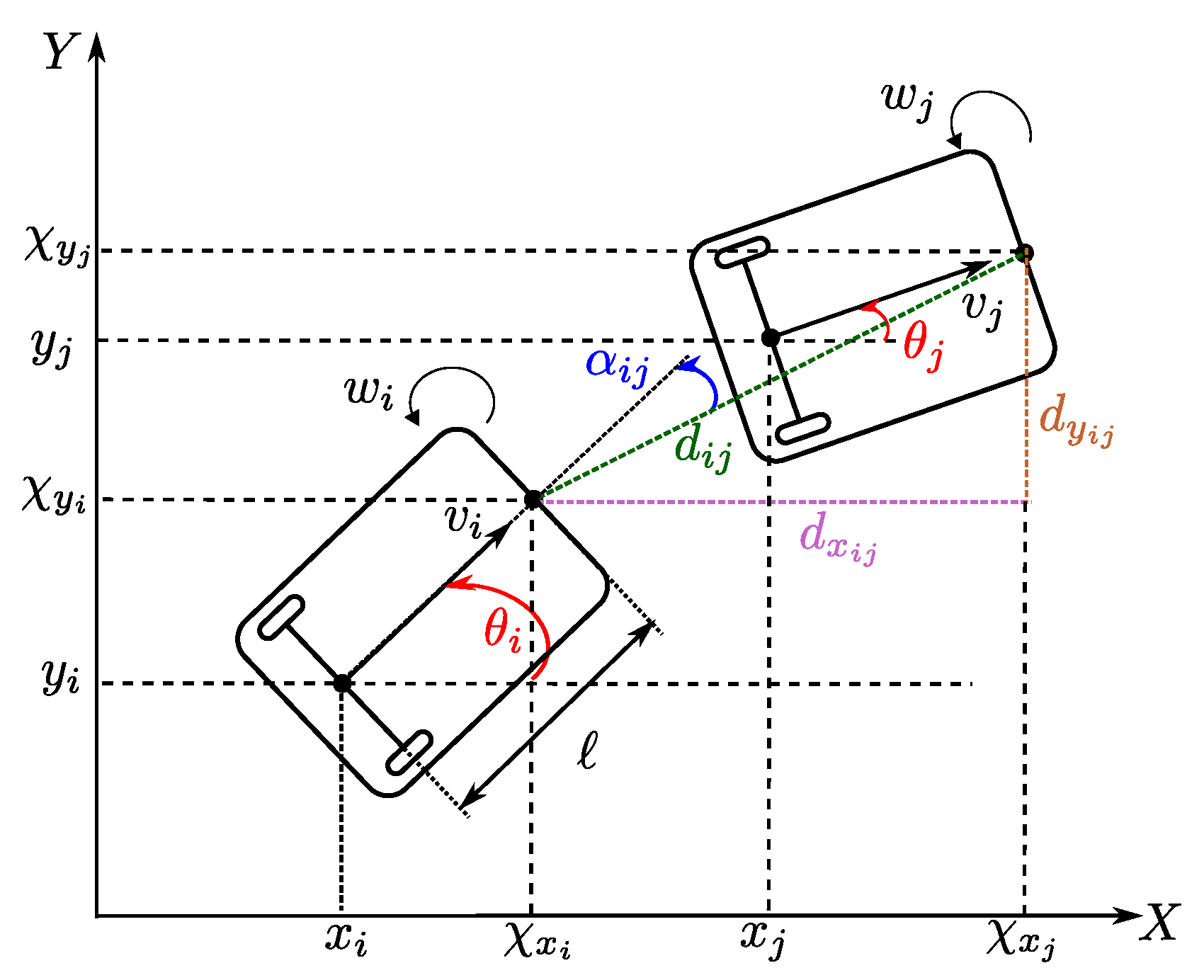
Abstract
:1. Introduction
1.1. Motivation
1.2. Related Works
1.3. Contribution
- It utilizes the robust ADRC scheme (with a custom error-based high-order ESO) that allows the follower agent to keep a desired distance and formation angle with respect to its own leader in spite the external disturbances, i.e., linear and lateral slipping parameters as well as unknown leader dynamics and velocities.
- It only depends on the distance and formation angle measurements.
- It is developed using solely a kinematic model based on the distance and the formation angle between a pair of robots, taking into account the front point of the differential-drive mobile robots.
2. Leader–Follower Problem
2.1. Considered Class of Systems
2.2. Problem Statement
- Leader tracks a prescribed trajectory, i.e.,where is the desired trajectory;
- Agent maintains a desired distance and a desired formation angle with respect to the agent , i.e.,where is the vector that contains the desired distance and the desired formation angle .
3. Proposed Control System
3.1. Leader–Follower Scheme Based on Distance and Formation Angle between the Agents
3.2. Followers Control Strategy
3.3. Leader Control Strategy
4. Experimental Validation
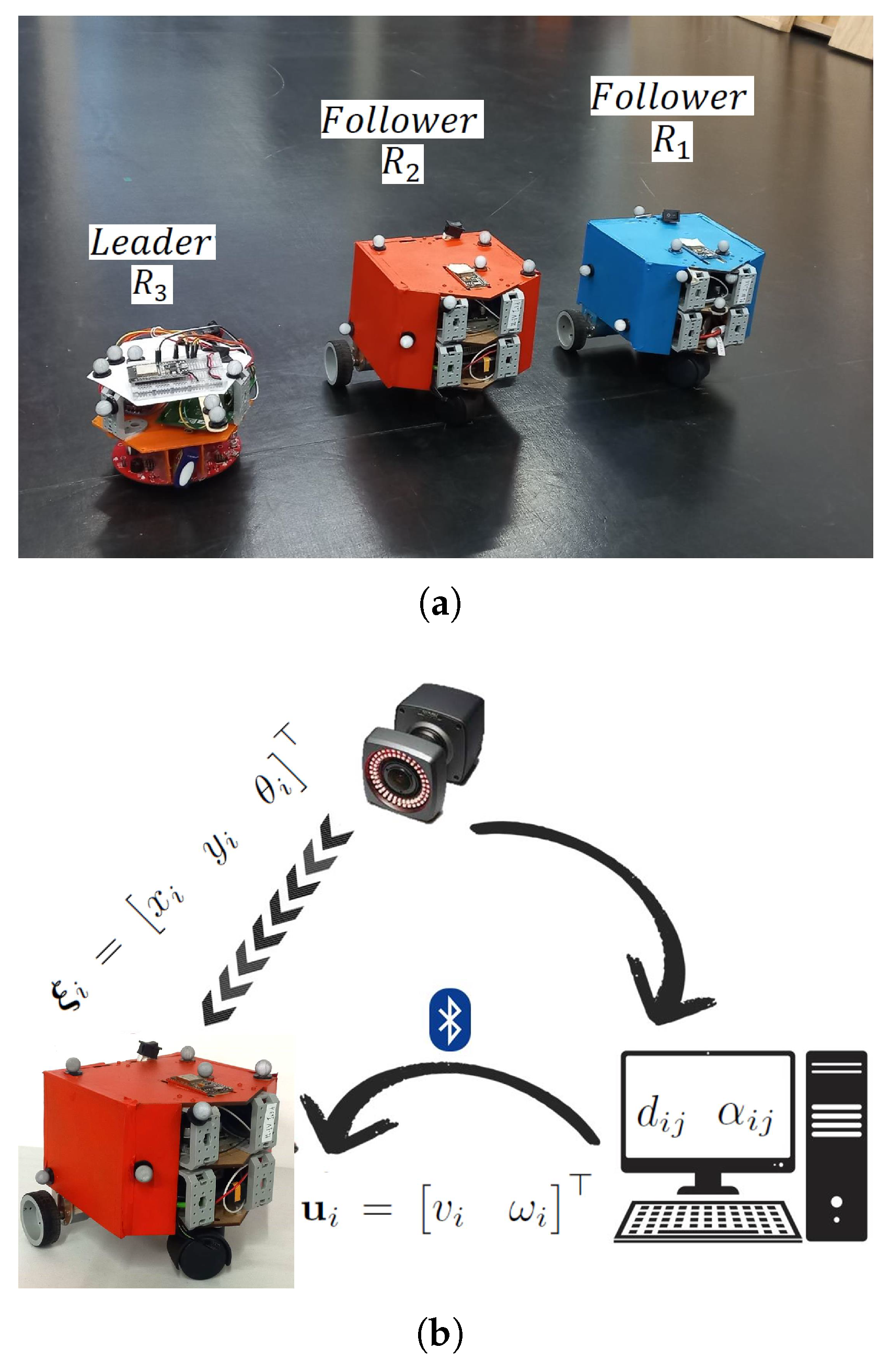
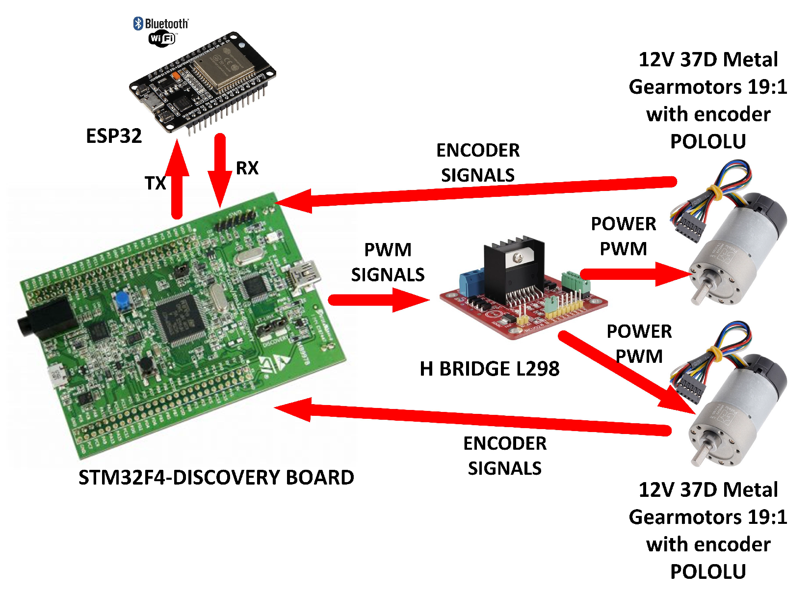
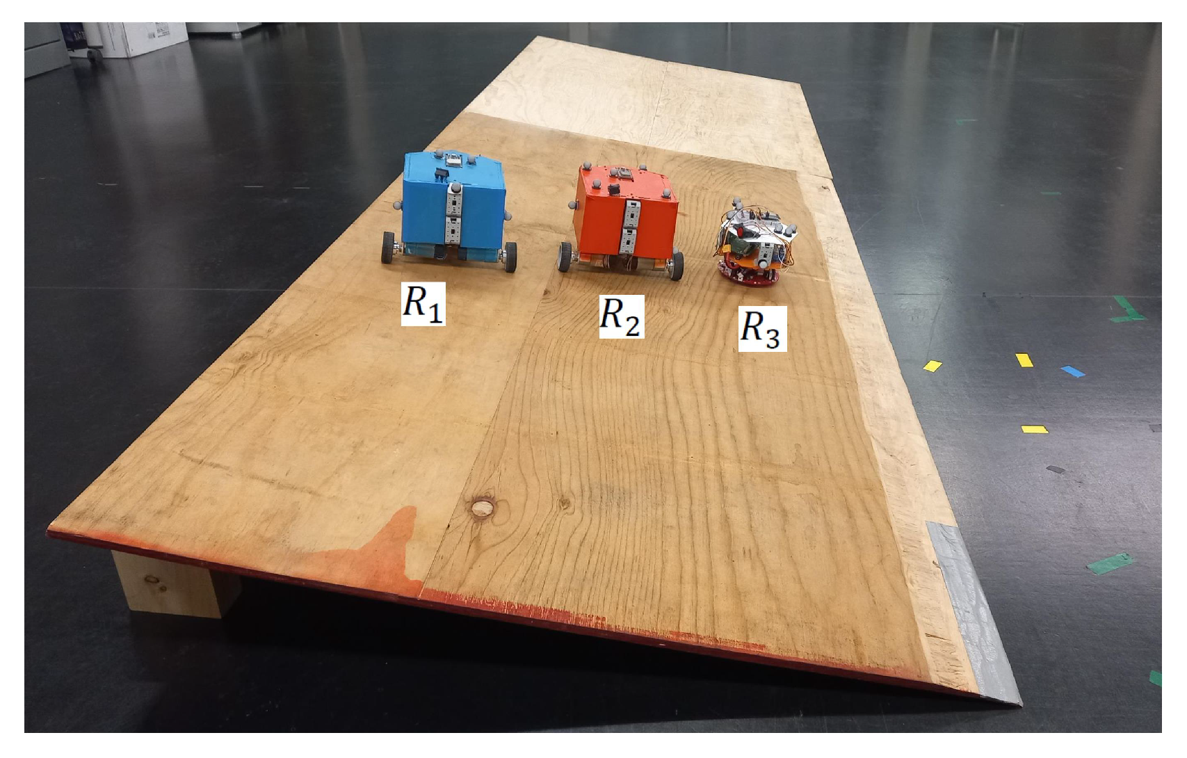
4.1. Experimental Platform
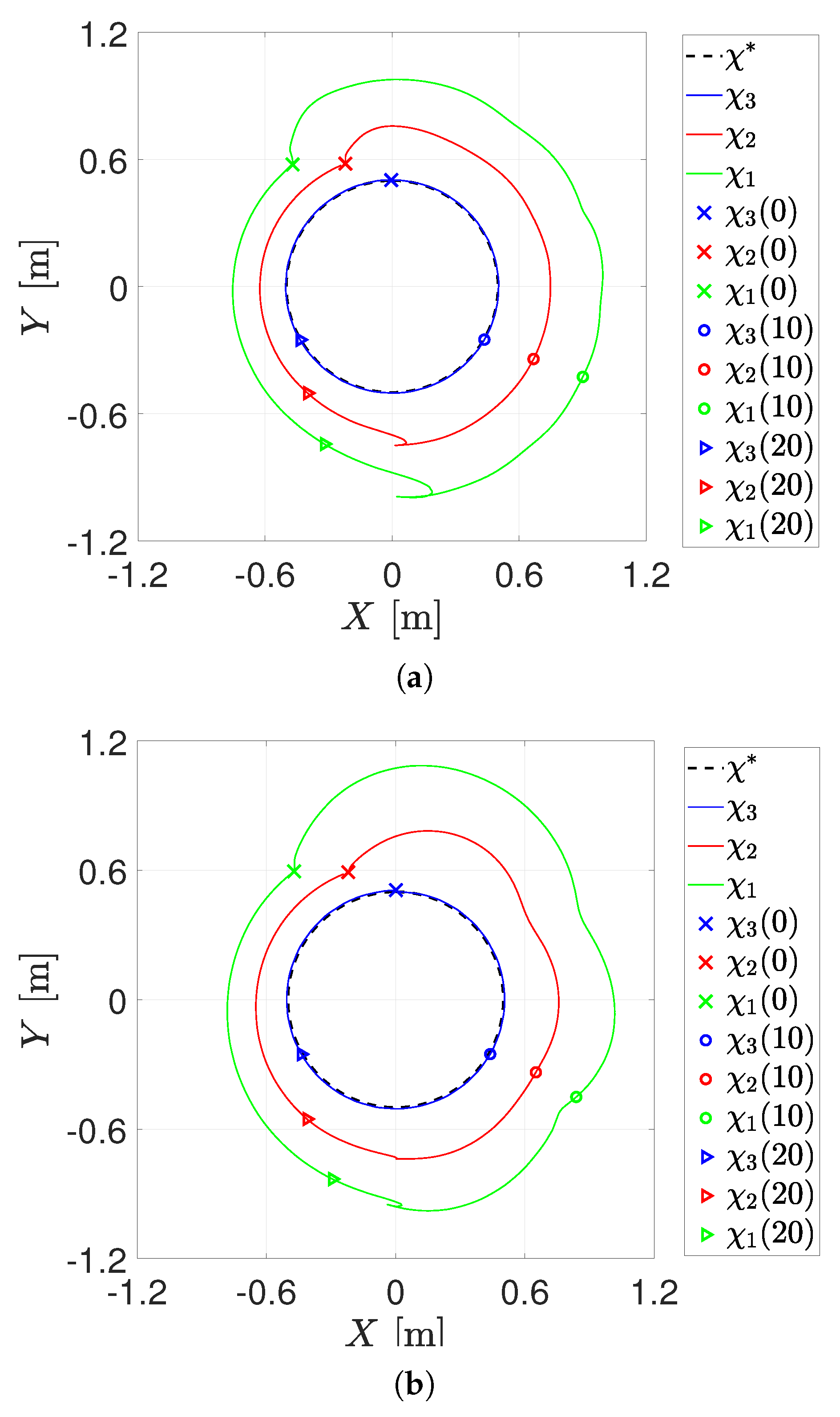
4.2. First Experiment
4.3. Second Experiment
5. Conclusions
Supplementary Materials
Author Contributions
Funding
Data Availability Statement
Conflicts of Interest
Abbreviations
| ADRC | Active Disturbance Rejection Control |
| PID | Proportional Integral Derivative Control |
| ESO | Extended State Observer |
| GPIO | Generalized Proportional Integral Observer |
References
- Yan, Z.; Jouandeau, N.; Cherif, A.A. A survey and analysis of multi-robot coordination. Int. J. Adv. Robot. Syst. 2013, 10, 399. [Google Scholar] [CrossRef]
- Feng, Z.; Hu, G.; Sun, Y.; Soon, J. An overview of collaborative robotic manipulation in multi-robot systems. Annu. Rev. Control 2020, 49, 113–127. [Google Scholar] [CrossRef]
- Ren, W.; Beard, R.W. Distributed Consensus in Multi-Vehicle Cooperative Control; Springer: Berlin/Heidelberg, Germany, 2008. [Google Scholar]
- Wang, X.; Li, S.; Yu, X.; Yang, J. Distributed active anti-disturbance consensus for leader-follower higher-order multi-agent systems with mismatched disturbances. IEEE Trans. Autom. Control 2016, 62, 5795–5801. [Google Scholar] [CrossRef]
- González-Sierra, J.; Hernández-Martínez, E.G.; Ferreira-Vazquez, E.D.; Flores-Godoy, J.J.; Fernandez-Anaya, G.; Paniagua-Contro, P. Leader-follower control strategy with rigid body behavior. IFAC-PapersOnLine 2018, 51, 184–189. [Google Scholar] [CrossRef]
- Wang, X.; Liu, W.; Wu, Q.; Li, S. A Modular Optimal Formation Control Scheme of Multiagent Systems With Application to Multiple Mobile Robots. IEEE Trans. Ind. Electron. 2022, 69, 9331–9341. [Google Scholar] [CrossRef]
- Hernández-Martínez, E.G.; Aranda-Bricaire, E. Trajectory tracking for groups of unicycles with convergence of the orientation angles. In Proceedings of the IEEE Conference on Decision and Control, Atlanta, GA, USA, 15–17 December 2010; pp. 6323–6328. [Google Scholar]
- Desai, J.P.; Ostrowski, J.P.; Kumar, V. Modeling and control of formations of nonholonomic mobile robots. IEEE Trans. Robot. Autom. 2001, 17, 905–908. [Google Scholar] [CrossRef] [Green Version]
- Deghat, M.; Shames, I.; Anderson, B.D.O.; Yu, C. Localization and Circumnavigation of a Slowly Moving Target Using Bearing Measurements. IEEE Trans. Autom. Control 2014, 59, 2182–2188. [Google Scholar] [CrossRef]
- Shames, I.; Dasgupta, S.; Fidan, B.; Anderson, B.D.O. Circumnavigation Using Distance Measurements Under Slow Drift. IEEE Trans. Autom. Control 2012, 57, 889–903. [Google Scholar] [CrossRef]
- Shao, J.; Tian, Y.P. Multi-target localization and circumnavigation control by a group of moving agents. In Proceedings of the IEEE International Conference on Control Automation, Ohrid, Macedonia, 3–6 July 2017; pp. 606–611. [Google Scholar]
- Boccia, A.; Adaldo, A.; Dimarogonas, D.V.; di Bernardo, M.; Johansson, K.H. Tracking a mobile target by multi-robot circumnavigation using bearing measurements. In Proceedings of the IEEE Conference on Decision and Control, Melbourne, Australia, 12–15 December 2017; pp. 1076–1081. [Google Scholar]
- Zhong, H.; Miao, Y.; Tan, Z.; Li, J.; Zhang, H.; Fierro, R. Circumnavigation of a Moving Target in 3D by Multi-agent Systems with Collision Avoidance: An Orthogonal Vector Fields-based Approach. Int. J. Control Autom. Syst. 2019, 17, 212–224. [Google Scholar] [CrossRef]
- Shen, D.; Sun, Z.; Sun, W. Leader-follower formation control without leader’s velocity information. Sci. China Inf. Sci. 2014, 57, 1–12. [Google Scholar] [CrossRef]
- Zhao, Y.; Zhang, Y.; Lee, J. Lyapunov and Sliding Mode Based Leader-follower Formation Control for Multiple Mobile Robots with an Augmented Distance-angle Strategy. Int. J. Control Autom. Syst. 2019, 17, 1314–1321. [Google Scholar] [CrossRef]
- Hua, C.C.; Liu, X.P. Delay-Dependent Stability Criteria of Teleoperation Systems with Asymmetric Time-Varying Delays. IEEE Trans. Robot. 2010, 26, 925–932. [Google Scholar] [CrossRef]
- Saha, O.; Dasgupta, P. A comprehensive survey of recent trends in cloud robotics architectures and applications. Robotics 2018, 7, 47. [Google Scholar] [CrossRef] [Green Version]
- Toris, R.; Kammerl, J.; Lu, D.V.; Lee, J.; Jenkins, O.C.; Osentoski, S.; Wills, M.; Chernova, S. Robot web tools: Efficient messaging for cloud robotics. In Proceedings of the IEEE/RSJ International Conference on Intelligent Robots and Systems (IROS), Hamburg, Germany, 28 September–3 October 2015; pp. 4530–4537. [Google Scholar]
- Diddeniya, I.; Wanniarachchi, I.; Gunasinghe, H.; Premachandra, C.; Kawanaka, H. Human–Robot Communication System for an Isolated Environment. IEEE Access 2022, 10, 63258–63269. [Google Scholar] [CrossRef]
- Panchi, F.; Hernández, K.; Chávez, D. MQTT Protocol of IoT for Real Time Bilateral Teleoperation Applied to Car-Like Mobile Robot. In Proceedings of the 2018 IEEE Third Ecuador Technical Chapters Meeting (ETCM), Cuenca, Ecuador, 15–19 October 2018; pp. 1–6. [Google Scholar]
- Han, J. From PID to active disturbance rejection control. IEEE Trans. Ind. Electron. 2009, 56, 900–906. [Google Scholar] [CrossRef]
- Sira-Ramírez, H.; Luviano-Juárez, A.; Ramírez-Neria, M.; Zurita-Bustamante, E.W. Active Disturbance Rejection Control of Dynamic Systems: A Flatness Based Approach; Butterworth-Heinemann: Oxford, UK, 2018. [Google Scholar]
- Herbst, G. Practical Active Disturbance Rejection Control: Bumpless Transfer, Rate Limitation, and Incremental Algorithm. IEEE Trans. Ind. Electron. 2016, 63, 1754–1762. [Google Scholar] [CrossRef] [Green Version]
- Madonski, R.; Shao, S.; Zhang, H.; Gao, Z.; Yang, J.; Li, S. General error-based active disturbance rejection control for swift industrial implementations. Control Eng. Pract. 2019, 84, 218–229. [Google Scholar] [CrossRef]
- Gao, Z.; Zheng, Q. Active disturbance rejection control: Some recent experimental and industrial case studies. Control Theory Technol. 2018, 16, 301–313. [Google Scholar]
- Madonski, R.; Herman, P. Survey on methods of increasing the efficiency of extended state disturbance observers. ISA Trans. 2015, 56, 18–27. [Google Scholar] [CrossRef]
- Wu, Z.H.; Zhou, H.C.; Guo, B.Z.; Deng, F. Review and new theoretical perspectives on active disturbance rejection control for uncertain finite-dimensional and infinite-dimensional systems. Nonlinear Dyn. 2020, 101, 935–959. [Google Scholar] [CrossRef]
- Zhang, X.; Zhang, X.; Xue, W.; Xin, B. An overview on recent progress of extended state observers for uncertain systems: Methods, theory, and applications. Adv. Control Appl. 2021, 3, e89. [Google Scholar] [CrossRef]
- Sira-Ramírez, H.; López-Uribe, C.; Velasco-Villa, M. Linear Observer-Based Active Disturbance Rejection Control of the Omnidirectional Mobile Robot. Asian J. Control 2013, 15, 51–63. [Google Scholar] [CrossRef]
- Ren, C.; Liu, R.; Ma, S.; Hu, C.; Cao, L. ESO Based Model Predictive Control of an Omnidirectional Mobile Robot with Friction Compensation. In Proceedings of the Chinese Control Conference, Wuhan, China, 25–27 July 2018; pp. 3943–3948. [Google Scholar]
- Ren, C.; Zhang, M.; Ma, S.; Wei, D. Trajectory Tracking Control of an Omnidirectional Mobile Manipulator Based on Active Disturbance Rejection Control. In Proceedings of the World Congress on Intelligent Control and Automation, Changsha, China, 4–8 July 2018; pp. 1537–1542. [Google Scholar]
- Fliess, M.; Lévine, J.; Martin, P.; Rouchon, P. Flatness and defect of non-linear systems: Introductory theory and examples. Int. J. Control 1995, 61, 1327–1361. [Google Scholar] [CrossRef] [Green Version]
- Michalek, M.M. Robust trajectory following without availability of the reference time-derivatives in the control scheme with active disturbance rejection. In Proceedings of the American Control Conference, Boston, MA, USA, 6–8 July 2016; pp. 1536–1541. [Google Scholar]
- Ramirez-Neria, M.; Madonski, R.; Shao, S.; Gao, Z. Robust tracking in underactuated systems using flatness-based ADRC with cascade observers. J. Dyn. Syst. Meas. Control 2020, 142, 091002. [Google Scholar] [CrossRef]
- Stankovic, M.; Madonski, R.; Manojlovic, S.; Lechekhab, T.E.; Mikluc, D. Error-Based Active Disturbance Rejection Altitude/Attitude Control of a Quadrotor UAV. In Advanced, Contemporary Control; Springer: Berlin/Heidelberg, Germany, 2020; pp. 1348–1358. [Google Scholar]
- Chen, S.; Chen, Z.; Zhao, Z. An error-based active disturbance rejection control with memory structure. Meas. Control 2021, 54, 724–736. [Google Scholar] [CrossRef]
- Ramírez-Neria, M.; Madonski, R.; Luviano-Juárez, A.; Gao, Z.; Sira-Ramírez, H. Design of ADRC for Second-Order Mechanical Systems without Time-Derivatives in the Tracking Controller. In Proceedings of the American Control Conference, Denver, CO, USA, 1–3 July 2020; pp. 2623–2628. [Google Scholar]
- Cui, M.; Huang, R.; Liu, H.; Liu, X.; Sun, D. Adaptive tracking control of wheeled mobile robots with unknown longitudinal and lateral slipping parameters. Nonlinear Dyn. 2014, 2014, 1811–1826. [Google Scholar] [CrossRef]
- Wang, D.; Low, C.B. Modeling and Analysis of Skidding and Slipping in Wheeled Mobile Robots: Control Design Perspective. IEEE Trans. Robot. 2008, 24, 676–687. [Google Scholar] [CrossRef]
- Li, Z.; Canny, J. Nonholonomic Motion Planning; Springer Science & Business Media: Berlin/Heidelberg, Germany, 1993. [Google Scholar]
- Spong, M.W.; Hutchinson, S.; Vidyasagar, M. Robot Modeling and Control; John Wiley & Sons: Hoboken, NJ, USA, 2020. [Google Scholar]
- Fareh, R.; Khadraoui, S.; Abdallah, M.Y.; Baziyad, M.; Bettayeb, M. Active disturbance rejection control for robotic systems: A review. Mechatronics 2021, 80, 102671. [Google Scholar] [CrossRef]
- Rouchon, P.; Fliess, M.; Lévine, J.; Martin, P. Flatness and motion planning: The car with n trailers. In Proceedings of the ECC’93, Groningen, The Netherlands, 28 June–1 July 1993; pp. 1518–1522. [Google Scholar]
- Gao, Z. Scaling and bandwidth-parameterization based controller tuning. In Proceedings of the American Control Conference, Denver, CO, USA, 4–6 June 2003; Volume 6, pp. 4989–4996. [Google Scholar]
- Ochoa-Ortega, G.; Villafuerte-Segura, R.; Luviano-Juárez, A.; Ramírez-Neria, M.; Lozada-Castillo, N. Cascade Delayed Controller Design for a Class of Underactuated Systems. Complexity 2020, 2020, 2160743. [Google Scholar] [CrossRef]
- Villafuerte, R.; Mondié, S.; Garrido, R. Tuning of proportional retarded controllers: Theory and experiments. IEEE Trans. Control Syst. Technol. 2012, 21, 983–990. [Google Scholar] [CrossRef]


Publisher’s Note: MDPI stays neutral with regard to jurisdictional claims in published maps and institutional affiliations. |
© 2022 by the authors. Licensee MDPI, Basel, Switzerland. This article is an open access article distributed under the terms and conditions of the Creative Commons Attribution (CC BY) license (https://creativecommons.org/licenses/by/4.0/).
Share and Cite
Ramírez-Neria, M.; González-Sierra, J.; Luviano-Juárez, A.; Lozada-Castillo, N.; Madonski, R. Active Disturbance Rejection Strategy for Distance and Formation Angle Decentralized Control in Differential-Drive Mobile Robots. Mathematics 2022, 10, 3865. https://doi.org/10.3390/math10203865
Ramírez-Neria M, González-Sierra J, Luviano-Juárez A, Lozada-Castillo N, Madonski R. Active Disturbance Rejection Strategy for Distance and Formation Angle Decentralized Control in Differential-Drive Mobile Robots. Mathematics. 2022; 10(20):3865. https://doi.org/10.3390/math10203865
Chicago/Turabian StyleRamírez-Neria, Mario, Jaime González-Sierra, Alberto Luviano-Juárez, Norma Lozada-Castillo, and Rafal Madonski. 2022. "Active Disturbance Rejection Strategy for Distance and Formation Angle Decentralized Control in Differential-Drive Mobile Robots" Mathematics 10, no. 20: 3865. https://doi.org/10.3390/math10203865