Kinematic Modelling for Hyper-Redundant Robots—A Structured Guide

Abstract

Obtaining mathematical equations to model the kinematics of a hyper-redundant robot is not intuitive and of greater difficulty than for traditional robots. Depending on the characteristics of the robot, the most appropriate methodology to approach the modelling may be one or another. This article provides a general overview of the different approaches there are when modelling a hyper-redundant cable-driven robot, while proposing a guide to help the novel researcher that approaches this field decide which methodology to apply when modelling a robot. After providing some definitions, a simple framework to understand all the underlying models is presented. Afterwards, the mathematical equations for the most important methods of modelling are developed. Finally, the proposal for a step-by-step tutorial is included, and it is exemplified by applying it to three real robots.

1. Introduction, Motivation and Definitions

In the 1960s, works with large robotic kinematic chains that involve a high number of degrees of freedom, also named hyper-redundant robots, had already started. The increase in the number of degrees of freedom allowed new configurations and innovative solutions for tasks. An example of the beginnings of hyper-redundant robotics was the Scripps Tensor Arm (1968) [1]. However, the increased difficulty in the control algorithms caused the investigation inside the field to stop in the 1970s. Once again, in the 1980s, Professor Hirose started developing new techniques and robots [2]. In 1990, the modal approximation method (based on approximating the robot’s backbone to a mathematically describable curve) appeared [3].

Between the years 2000 and 2010, the investigation continued, both in the theoretical approach (for example, some works of Walker: [4,5,6]) and the applications, which can be found in the bibliography revisions made by Webster, Jones and Bryan [7]. Currently, the work that is being conducted in the hyper-redundant robotics field continues with this tendency. For example, new algorithms are being searched in order to efficiently solve their kinematics [8,9,10,11,12] while new applications are also being proposed [13,14].

The number of publications for the novel researcher in this field may be overwhelming. Some concepts might be confusing, due to the wide range of configurations that exist. There are many mathematical proposals to obtain different models, either spread around publications or treated without any apparent similarities. It is not difficult to imagine that some might wonder where to begin when modelling a hyper-redundant robotic arm. Some efforts are being made to provide a classification of the different kinematic models, comparing them through some benchmark studies [15] or providing a brief comparison between kinematic models for soft robots [16]. However, a framework for novel researchers is not provided, and they rely on some previous knowledge of how modelling is tackled.

Therefore, this article tries to give an overview of the most relevant and efficient techniques that currently exist and to provide a certain general framework to approach this task. It also proposes some criteria to select the most appropriate modelling methodology and applies them in some real examples.

To do so, a simple classification of hyper-redundant robots is adopted as one of the main criteria for choosing a certain method. Afterwards, some generalities on cable-driven hyper-redundant modelling are described. Then, these generalities are analysed on certain algorithms: Denavit–Hartenberg, the PCC (Piecewise Constant Curvature) method or the LSK (Linearised Segment Kinematics) equations. Additionally, and for completeness, a possible algorithm for solving the inverse kinematics is also explained: the Natural-CCD algorithm. Finally, the proposal of the flow diagram is explained and validated.

1.1. Definitions

In order to establish a kinematic model for “hyper-redundant robots”, it must first be established what is considered as such. For this tutorial, the criterion proposed by Martin et al. [8] is accepted, which distinguishes between discreet robots, redundant robots and hyper-redundant robots. Other authors do not offer a numerical difference between such cases [17].

To completely define the position and orientation of a rigid body in a vector space defined in ${\mathbb{R}}^m$, the number of degrees of freedom required is given by Equation (1).

$$DO{F}_{{\mathbb{R}}^m}=\frac{m(m+1)}{2}$$

(1)

In particular, for the 2D space ${\mathbb{R}}^2$, $m=2\Rightarrow DOF=3$, and for the 3D space ${\mathbb{R}}^3$, in which most robots work, $m=3\Rightarrow DOF=6$.

Taking this into account, a possible classification of robots can be established:

• Nonredundant robot: Any robot whose degrees of freedom are fewer than or equal to $DO{F}_{{\mathbb{R}}^m}$, that is, the minimal number of degrees of freedom to completely define the position and orientation of the robot endpoint.
• Redundant robot: A robot with more than $DO{F}_{{\mathbb{R}}^m}$ degrees of freedom. They are ensured to be capable of reaching a certain state through different joint configurations since there are infinite solutions for each state.
• Hyper-redundant robots: A robot with more than twice the minimal degrees of freedom required to completely define the endpoint state ($DOF\ge 2·DO{F}_{{\mathbb{R}}^m}$).

This work focuses exclusively on hyper-redundant robots. However, given the exceptional breadth of this field, it exclusively refers to cable-driven hyper-redundant robots (from now on, CDHR). These particular robotic arms are formed by a series of sections delimited by discs, to some of which several cables are fixated. The modification of the cables’ length, mostly achieved by motors, are the actuators responsible for the robot’s movement. Hyper-redundancy is achieved by combining different sections with several cables attached to them.

1.2. Classification of CDHR

Once the concept of hyper-redundant cable-driven robots can be clearly delimited, it is desirable to establish a classification of which types can be found inside this set. To do so, several approaches could be adopted. Nevertheless, due to the final objective of achieving a step-by-step methodology to obtain a model for the robot, the following classification is used, which later makes it easier to find the desired equations for each case.

To do so, the concept of backbone should be introduced. The backbone of a CDHR is the internal support that joins the different discs together and that holds the weight of the robot itself. Using this new definition, three big sets of robots are suggested: discreet hyper-redundant robots, constant curvature continuous robots and other continuous robots. The features that distinguish each group are:

(1)

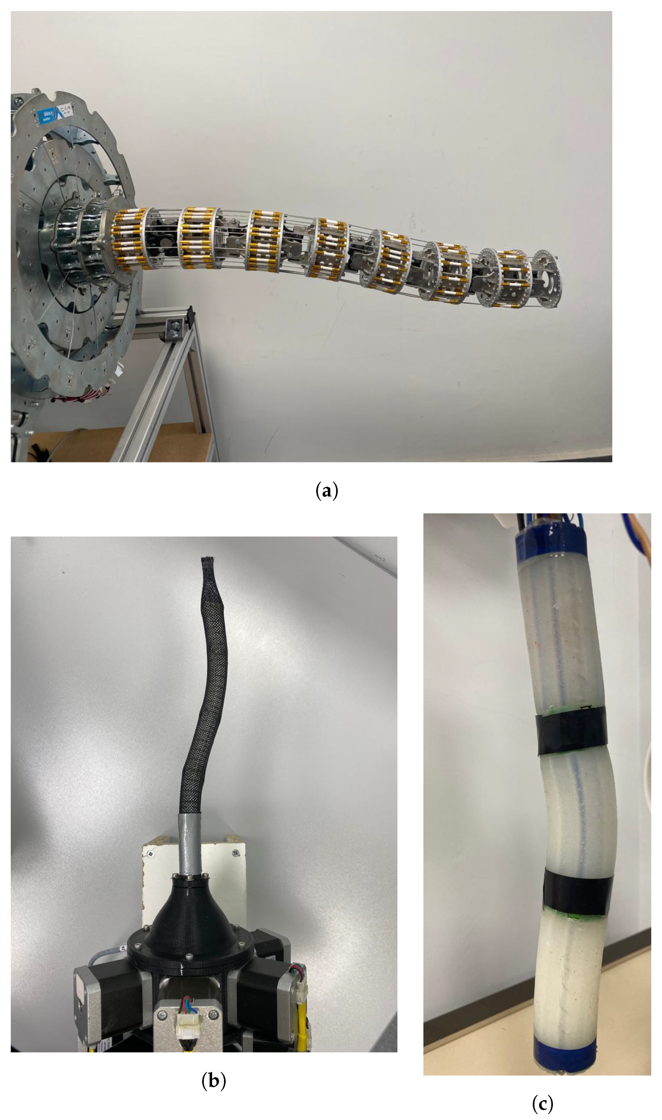
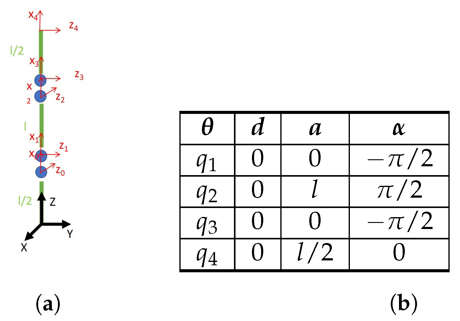
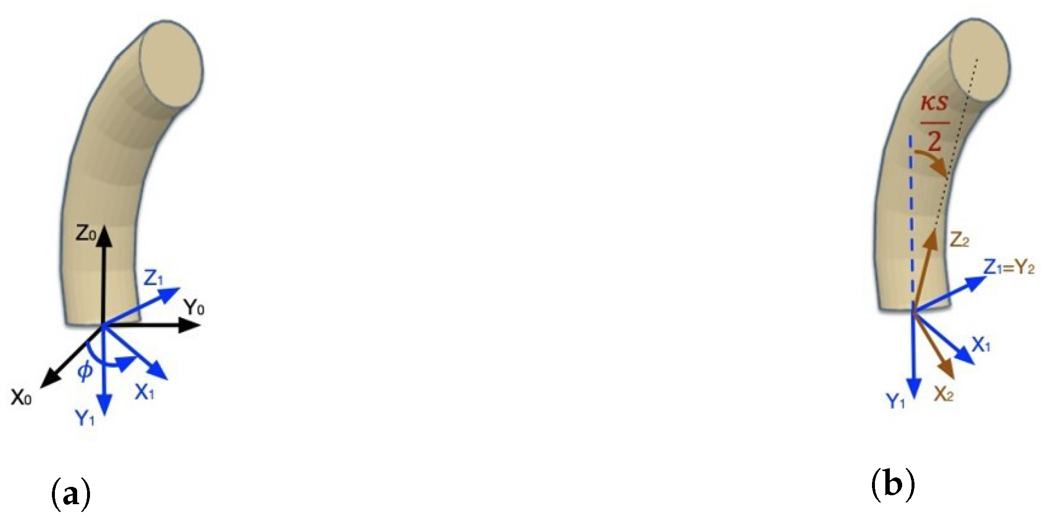
Discreet Hyper-Redundant Robots: The classical set of hyper-redundant robots and the most used in the origins of this field. Its main characteristic is that discreet robots are composed of a succession of rigid sections, joined together by, normally, one or two degree-of-freedom joints. The rigidity of the sections makes it possible to use traditional robotics techniques to obtain their kinematic model. MACH-I [14] (see Figure 1a) or Series II, X125 System from OC Robotics [18] are two examples of discreet hyper-redundant robots.

(2)

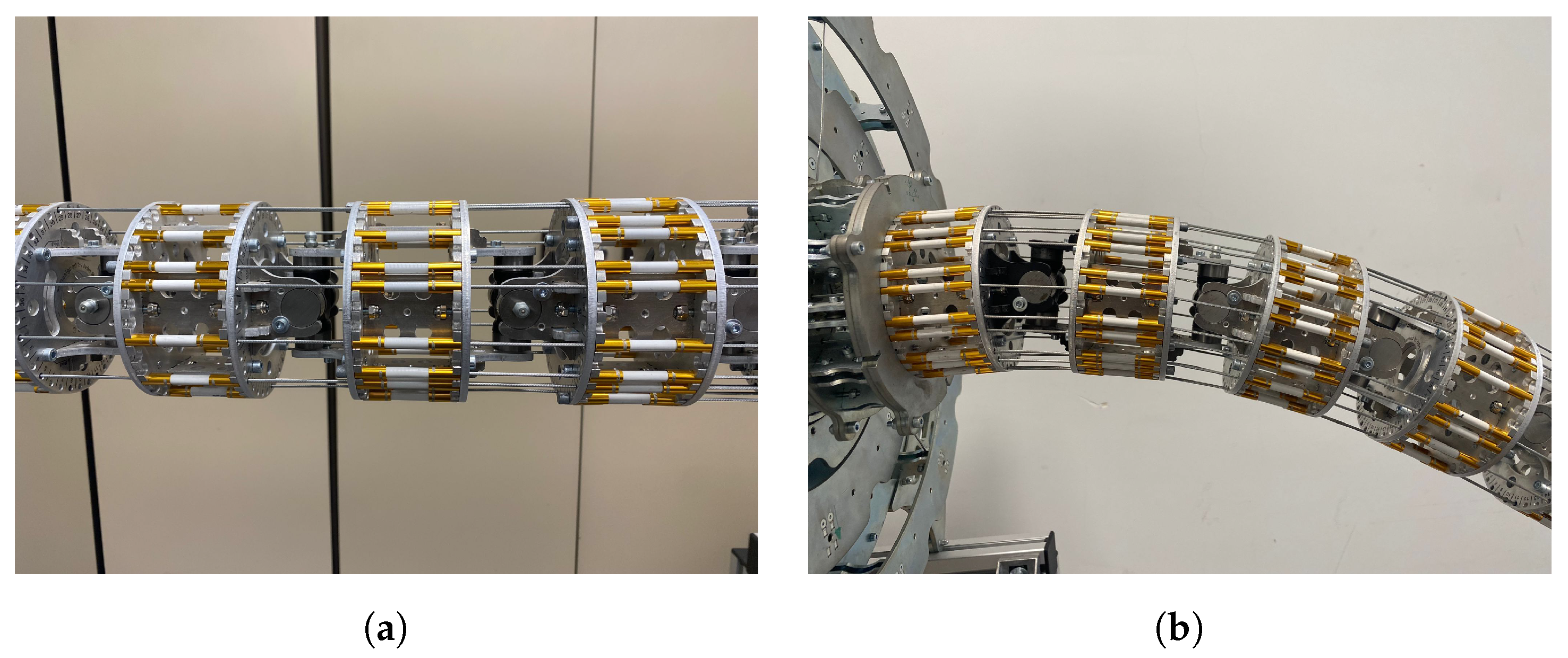
Constant Curvature Continuous Robots: in this group, we include any robot whose sections’ backbone can be mathematically modelled as a constant curvature segment. Therefore, actual continuous robots (soft robots, for example) might be included in this group, but also robots with discreet joints and deformable sections that form a curve. They are mathematically more challenging, but due to the assumption of constant curvature, their equations can be analytically obtained. Examples of this group of robots are the Elephant Trunk by Hannan and Walker [19] or Pylori-I (see Figure 1b), a pivotal discs CDHR [20].

(3)

Other Continuous Robots: In some cases, due to an excess of forces either in the backbone of the robot (excessive distributed weight) or in the endpoint, the constant curvature hypothesis cannot be applied. These cases are more difficult to manage, and they often imply using numerical methods to solve the constitutive equations of the robot. However, since this is a dynamic condition, they are morphologically equivalent to constant curvature robots (either with joints and deformable sections or soft robots). Most soft robots (such as Ruan [21], see Figure 1c, or Kyma [22]), specially those made by polymeric materials, need this kind of kinematic model.

2. Kinematic Modelling Stages for CDHR

In order to have an adequate base for CDHR robots’ kinematic modelling, several general aspects must be taken into account. Robot kinematics are affected by the characteristics they have. Once the previous classification is clear, general knowledge of the different steps for kinematic modelling is given so as to ease the introduction to the topic for newcomers.

2.1. Definitions and Nomenclature for the Kinematic Problem

The final objective of kinematic modelling is establishing the mathematical relationship between the state of the global robot’s structure at time t with the cable lengths at the same time instant. In the end, the degrees of freedom that can be managed are the lengths of these cables, and through them, the robot is positioned.

Some basic definitions are needed for developing the mathematical equations for hyper-redundant robots:

• The definition of the whole robot’s structure (the position of each of its points in space) is named the robot configuration.
• The discs (or equivalent physical structures) of the robot to which the cables are fixed are called active discs.
• The discs with no cables attached but that are crossed by them are called passive discs.
• Except as otherwise specified, the section of the robot is considered as the portion of the robot between two consecutive active discs.
• The determination of the position of each one of the infinite points of a certain section is named the section’s state. It can be represented in different ways depending on the type of robot or the chosen model (a vector, a matrix, etc.).
• The endpoint of a section is the theoretical point that represents the ending of a certain section of the robot. Although it could be arbitrarily defined, in this work the usual convention of the geometric centre of the ending disc is chosen. The endpoint of the robot would then be the last section’s endpoint.

Using these basic concepts, the kinematic problem can be mathematically presented as a transformation between reference systems. One global reference frame can be defined at the centre of the robot’s first disc, with its z axis perpendicular to it and pointing towards the next disc. Afterwards, a reference frame can be defined for each active disc, as well as for the endpoint of the robot. As sections are delimited by active discs, these reference frames represent the beginning and the end of a certain section.

The transformation between these reference frames is the essential tool to solve the kinematics: the simplifying hypotheses of many models, by approximating the robot to a defined shape, enables representing the state of the whole section through the information of its endpoint relative to its origin.

In addition to these concepts and definitions, a general naming convention is presented here, which is maintained throughout the whole article:

• The total number of sections of the robot is named n.
• The index k is used when referring to any particular section.
• The total number of cables or tendons the robot uses is named f.
• The endpoint of the robot is indicated with a subindex e.

2.2. Direct Kinematics

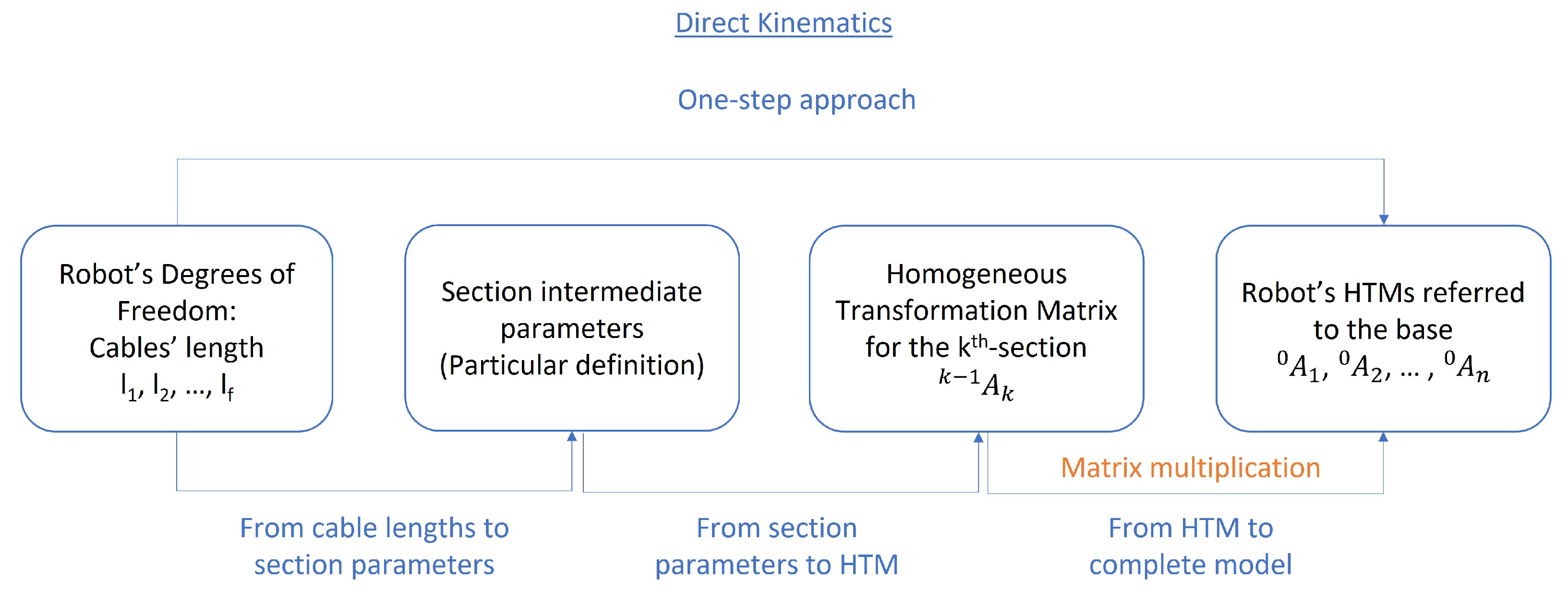
Direct kinematics in CDHR robots tries to find the relationship between the existing degrees of freedom (cables’ length) with the complete robot state at each moment. Let $\overrightarrow{x_1},\overrightarrow{x_2},\cdots ,\overrightarrow{x_n}$ be the states of each of the sections for a CDHR, represented as vectors of parameters. Due to hyper-redundancy, finding a direct solution in one step (from $l_1,l_2,\cdots ,l_n$ to $\overrightarrow{x_1},\overrightarrow{x_2},\cdots ,\overrightarrow{x_n}$) is a very complex task. Often, either simplification hypotheses must be assumed or numerical methods are applied [8]. Therefore, in most cases, the simplification hypotheses allow dividing the model into several steps.

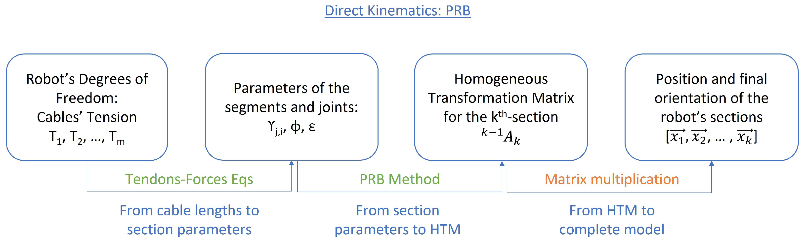
These simplifications usually make it possible to represent the state of the section with a finite set of intermediate parameters. For example, sometimes the pose (position and orientation) of the endpoint of a section is enough, considering a certain hypothesis, to represent the position of all its infinite points. The intermediate parameters can finally be inserted into a Homogeneous Transformation Matrix (HTM) between the origin of the section and its endpoint to have the mathematical representation of such section’s state. The set of all the HTMs for each section then represents the robot configuration. Therefore, this is the system used throughout the paper (unless specifically stated otherwise), ${}^i{A}_j$ being the HTM for section j referenced to section i.

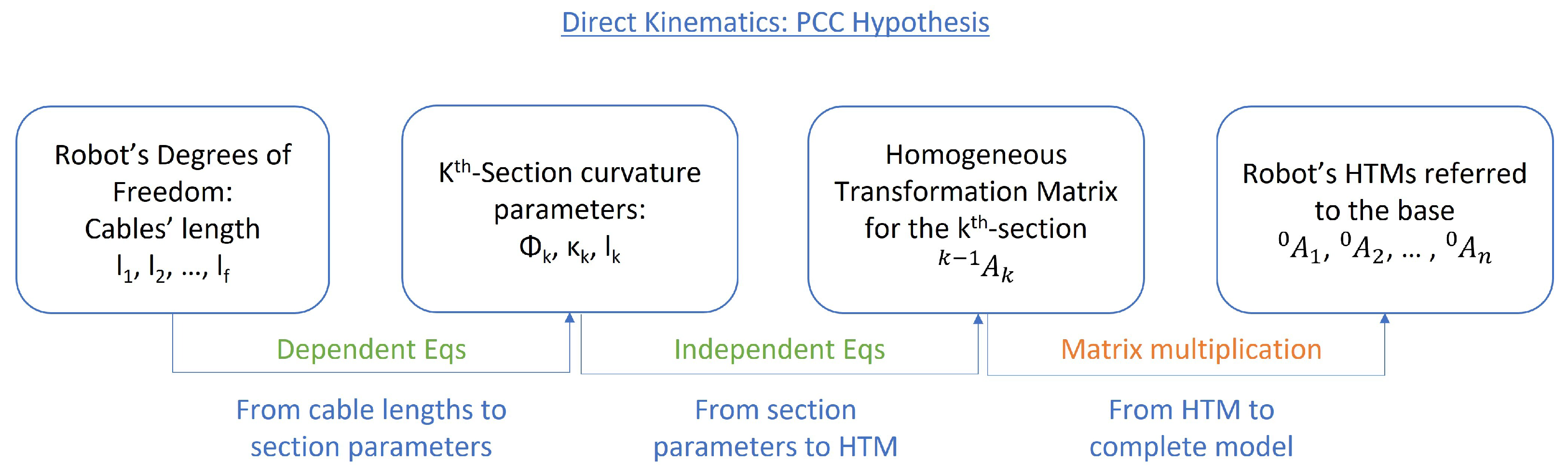
For this article, the schematic found in Figure 2 is used as a basis to classify the different direct-kinematic models. As stated, the last step of this theoretical framework is based on multiplying Homogeneous Transformation Matrices (HTMs) to obtain each section’s state referenced to the global frame. The other two steps are conditioned by the simplification hypothesis applied to the robot.

Usually, the first step is completely dependent on the robot being modelled (and as such, it relies on the engineer’s skills to obtain a mathematical relationship). The second step is frequently standard, and equations are already available in the bibliography. Throughout this paper, it is explained how each one of the mathematical hypothesis are fitted into this view of hyper-redundant kinematics.

2.3. Inverse Kinematics

The inverse kinematic problem consists in obtaining the necessary cable lengths required to achieve a certain robot configuration. As far as this article is concerned, inverse kinematics also involve determining a possible configuration for the robot when only the endpoint’s position, given certain spatial coordinates, is known. Inverse kinematics are inherently complex in robots with a high number of serial degrees of freedom: the state or configuration of each joint (that is, the angle rotated by each DOF about a certain origin) affects the configuration of all subsequent joints. Due to the nature of hyper-redundant robots, which have many degrees of freedom, inverse kinematics is a challenge [7].

The first question that might be asked is which spatial coordinates should be used for the inverse kinematics. Representing the pose (position and orientation) of a rigid solid in space requires six degrees of freedom. However, most models presented here use certain hypotheses that reduce the number of degrees of freedom per section. Moreover, the most common robotic morphologies currently studied used, at most, three or four cables per section.

In this work, we use a three degrees of freedom standard as the input of the inverse kinematics. Many morphologies use three independent cables, and those who use four cables usually involve redundancies between them, effectively reducing this number. For simplicity, the three Cartesian coordinates are used (${\left[\begin{array}{ccc}x& y& z\end{array}\right]}^t$), but orientation parameters could also be considered. Geometric relationships could then be applied to transform the equations between these two cases. In robots with fewer degrees of freedom per section, further restrictions have to be applied, as addressed in Section 7.

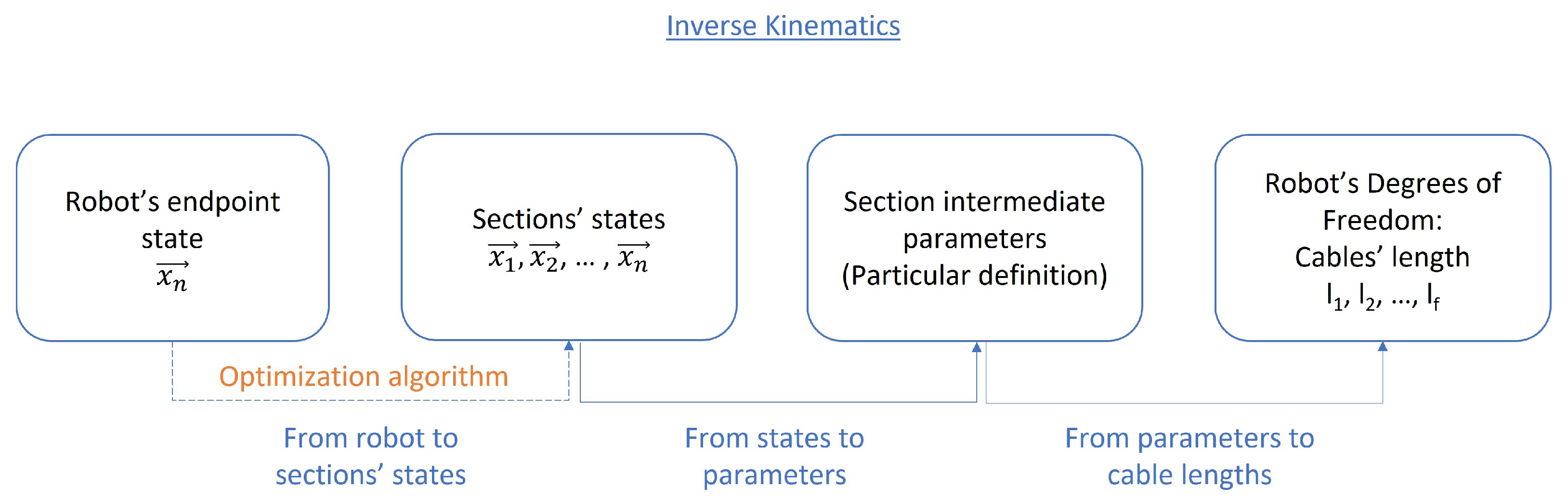
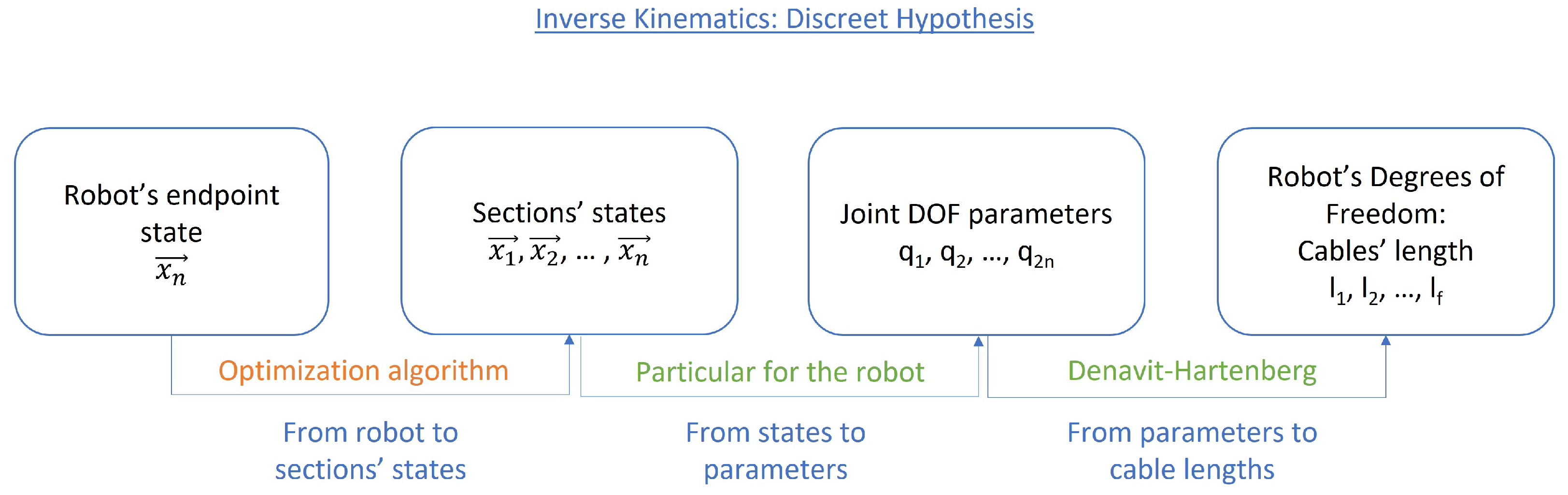
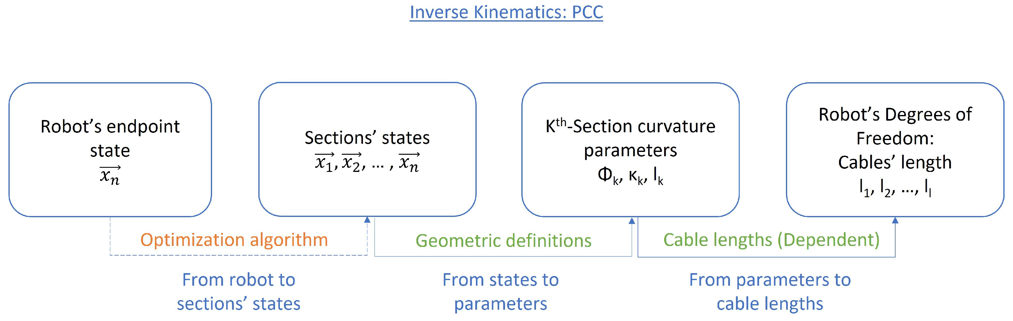
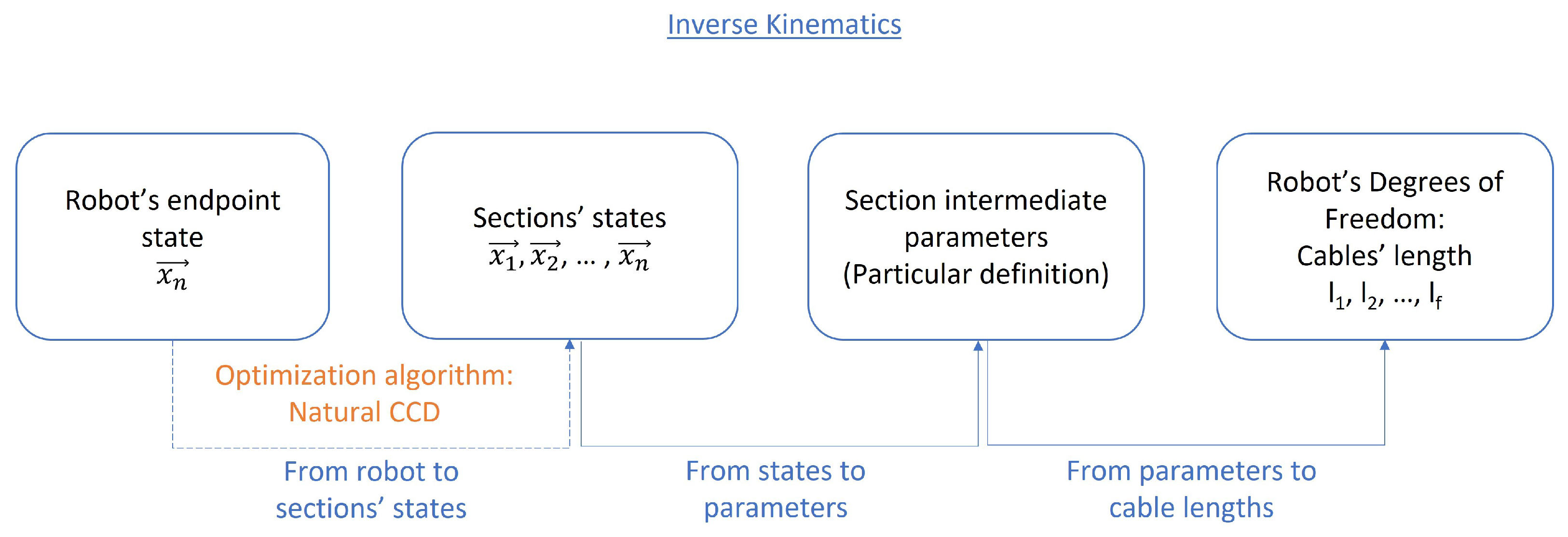
To obtain the inverse kinematic equations, an equivalent process to that of the direct kinematics is followed. The global problem is divided into various steps, which are particularised depending on the chosen simplifying hypothesis (See Figure 3). Once again, this diagram is used as the main guideline throughout the article for inverse kinematics.

The first step, the optimisation algorithm, is completely independent of the other tasks. It has been thoroughly studied in many papers, using many different techniques ([23,24,25]). The objective is to obtain a series of orientations and positions for each robot section that allows the robot to reach the endpoint goal.

In general, this step uses algorithms that work independently of the robot’s configuration definition (how the generalised coordinates are defined), since they model sections as reference systems and do not need specific information. Since the problem has infinite solutions, these algorithms typically try to optimise a certain value iteratively to obtain one solution. One example of such algorithms is the CCD algorithm or its improved version, the Natural-CCD [26], which is described further on. If the robot configuration is already given for a certain problem, this first step can be omitted.

The further steps depend on the chosen model for each particular robot. They are detailed for each hypothesis but include a transformation from the section’s state (usually the endpoint’s pose is enough, as stated in Section 2.1), to certain intermediate parameters. By using them, the cable lengths are found.

3. Discreet Hypothesis: Denavit–Hartenberg Method

3.1. Applying the Hypothesis

The first simplification hypothesis that is introduced is the discreet hypothesis. It is based on modelling the robot as a succession of perfectly distinguished 1 DOF or 2 DOF joints. It is the simplest of models, but it can be applied to many hyper-redundant robots. In particular, whenever the discreet hypothesis is acceptable, the Denavit–Hartenberg method is a very useful tool to obtain the equations: it is a systematic and well-known technique [27].

The method, which is briefly explained below, directly affects the second step for direct kinematics (see Figure 4). It fixes each of the joints’ DOF as the section parameters, and it gives a relationship from state parameters to HTMs. Only the first step is left unspecified: as stated in Section 2.2, it is highly dependent on the specific geometry of the robot, and cannot be presented in a completely general method.

Inverse kinematics are also affected by the discreet hypothesis, and the Denavit–Hartenberg method can also be used to obtain a procedure for inverse kinematics (see Figure 5). In this case, the relationship from states to parameters has to be obtained for the particular robot. However, once the parameters are available, the HTMs can be obtained for each section using the Denavit–Hartenberg method. Applying successive transformations to the cables’ endpoints in each section gives their position in space, which can be used to deduce their lengths. This procedure is applied to an example in Section 8.1.

3.2. Method Explanation

The Denavit–Hartenberg algorithm was proposed by Denavit and Hartenberg in the 20th century and used matrix linear algebra to obtain a kinematic model for a joint chain [27]. It is based on selecting a series of reference systems that have a simple relationship between them, reducing the six DOF of a 3-D space into four basic transformations. Using this method, a direct kinematic model can easily be found for a discreet succession of joints.

The key to applying this method is defining several reference systems: one for the robot’s base and one for each of the links between joints. Then, the transformation between successive reference systems is obtained by the combination of four movements: rotation of $\theta$ around the z axis, translation of d along the z axis, translation of a along the x axis and rotation of $\alpha$ around the x axis. The variable affected by the joint would be $\theta$ in the case of a rotation joint or d for a translation joint, the other three parameters being dependent on the robot’s geometry.

This algorithm is very popular in industrial robots, as serial configurations are very frequent in this field. The application to discreet hyper-redundant robots is direct since they are usually built as several serial one or two DOF joints. The method is independent of the final number of joints, and thus can be considered a general methodology for such discreet robots.

For the two DOF joints, it is common to divide it into two Denavit–Hartenberg reference systems but with the same origin (only the orientation would change). For each one DOF joint, a transformation matrix would then be obtained:

$$\begin{array}{c}\hfill {}^{k-1}{\mathit{A}}_k={\mathit{Rot}}_z\left({\theta }_k\right)\mathit{T}(0,0,d_k)\mathit{T}(a_k,0,0){\mathit{Rot}}_x\left({\alpha }_k\right)\\ \hfill =\left[\begin{array}{cccc}cos{\theta }_k& -cos{\alpha }_{k}sin{\theta }_k& sin\left({\alpha }_k\right)sin{\theta }_k& a_{k}cos{\theta }_k\\ sin{\theta }_k& cos{\alpha }_{k}cos{\theta }_k& -sin{\alpha }_{k}cos{\theta }_k& a_{k}sin{\theta }_k\\ 0& sin{\alpha }_k& cos{\alpha }_k& d_k\\ 0& 0& 0& 1\end{array}\right]\end{array}$$

(2)

Afterwards, by multiplying the matrices for each joint one after the other, the various endpoints would be achieved. This is very useful since it allows to combine these matrices in different ways, so that positions or velocities might be directly transformed from an arbitrary joint to another one, only multiplying by the desired transformations.

Since the Denavit–Hartenberg method is extensively described in the academic world (for example, in Ref. [28] or in Ref. [7]), the method is not thoroughly explained here. However, a simple example is shown, and it could be easily extended for discreet hyper-redundant robots. A robot with two joints, each of them with two DOF, would be then modelled as seen in Figure 6a,b.

With these parameters, the different equations for the reference systems would be obtained as:

$${}^B{\mathit{A}}_0=\mathit{T}(0,0,l/2){\mathit{Rot}}_y(-\pi /2)$$

$${}^0{\mathit{A}}_1={\mathit{Rot}}_z\left(q_1\right)\mathit{T}(0,0,0)\mathit{T}(0,0,0){\mathit{Rot}}_x(-\pi /2)$$

$${}^1{\mathit{A}}_2={\mathit{Rot}}_z\left(q_2\right)\mathit{T}(0,0,l)\mathit{T}(0,0,0){\mathit{Rot}}_x(\pi /2)$$

$${}^2{\mathit{A}}_3={\mathit{Rot}}_z\left(q_3\right)\mathit{T}(0,0,0)\mathit{T}(0,0,0){\mathit{Rot}}_x(-\pi /2)$$

$${}^3{\mathit{A}}_4={\mathit{Rot}}_z\left(q_4\right)\mathit{T}(0,0,l)\mathit{T}(0,0,0){\mathit{Rot}}_x\left(0\right)$$

$${}^B{\mathit{A}}_4{=}^B{\mathit{A}}_0{·}^0{\mathit{A}}_1{·}^1{\mathit{A}}_2{·}^2{\mathit{A}}_3{·}^3{\mathit{A}}_4$$

(3)

As stated before, this method is perfectly valid when joints can be easily distinguished, therefore classifying the robot as a discreet hyper-redundant robot. However, continuous robots such as Ruan [22] need further mathematical mechanisms to model their state.

4. PCC Hypothesis—Piecewise Constant Curvature

Piecewise Constant Curvature (PCC) kinematics is based on the assumption that the robot can be divided into a finite number of constant curvature arcs [7]. This is a desirable hypothesis in continuous hyper-redundant robots and can be successfully applied to many of them. Generally, the conditions for accepting such a hypothesis are, firstly, negligible effects of the gravity force and secondly, assuming the sections to which cables are attached are fixed to the backbone, allowing the robot to bend and producing a negligible friction [29].

Each of the robot’s constant curvature arcs is called the robot’s sections (as opposed to slices, which refer to the area defined by the slice of the robot at a certain point of the backbone). These sections usually correspond to the extent of the robot between two active slices.

4.1. Direct Kinematics

In Figure 7, the application of the PCC hypothesis to the theoretical framework previously established for direct kinematics is presented. The first determination that can be made is the parameters for the hypothesis. When accepting the constant curvature hypothesis, each of the robot’s sections can be modelled through three values: curvature $\kappa$, azimuthal angle $\varphi$ and the arc length l.

Having determined the section parameters, the two transformations that are left are a robot-dependent transformation (from cable lengths to section parameters), highly dependent on the morphology, and some robot-independent equations (from state parameters to HTM) that are valid for any robot. Both are examined in more detail.

4.1.1. Independent Transformation—Geometric Method

In this section, the second transformation is obtained: the mathematical equations for the kinematic model of a single section k are found by using geometrical relationships [7,30], even though alternative methods could be used to reach the same mathematical result (as seen in the next section). For clarity, given these formulae refer to a single section, the subindex k is omitted in the equations.

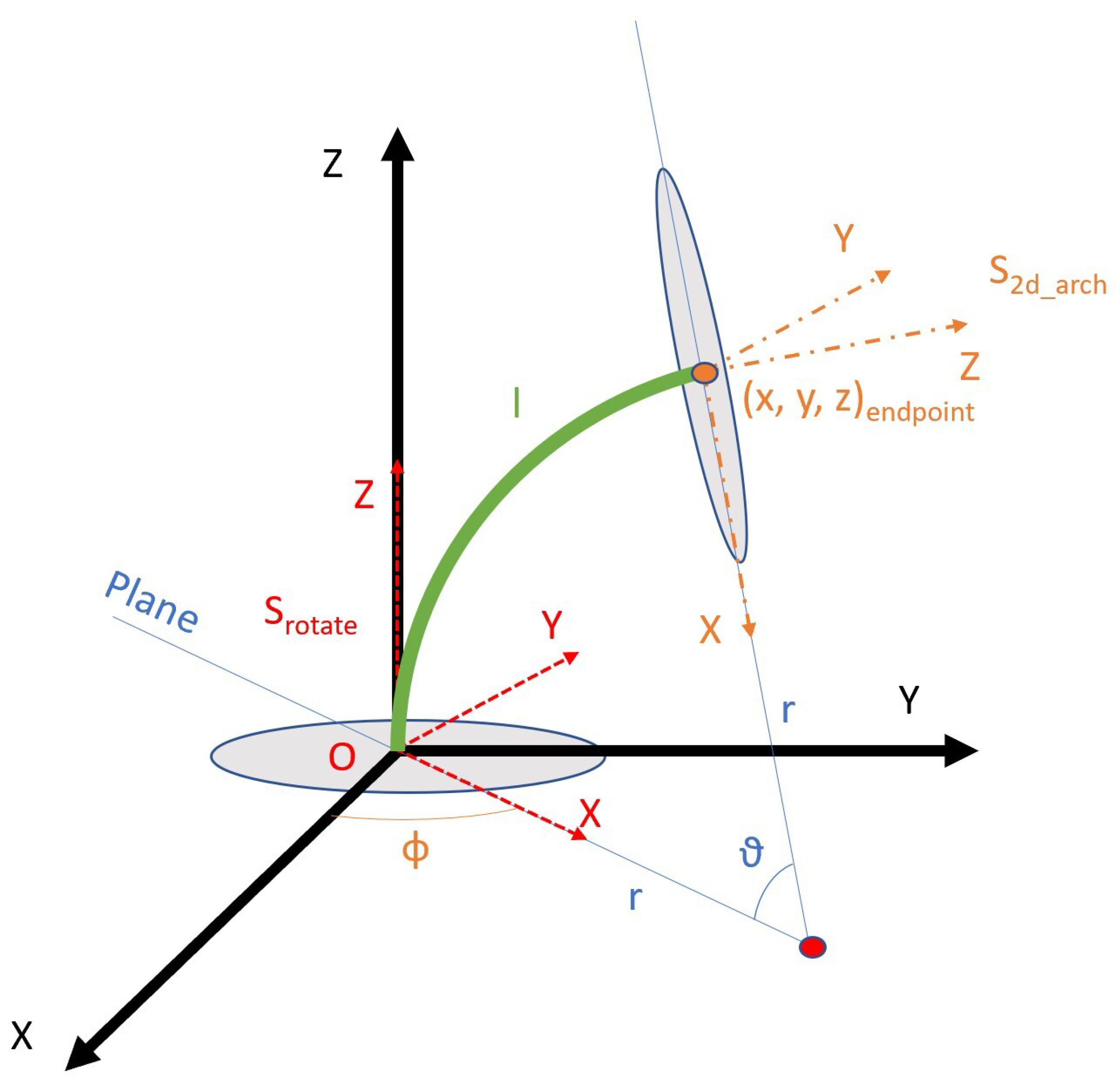
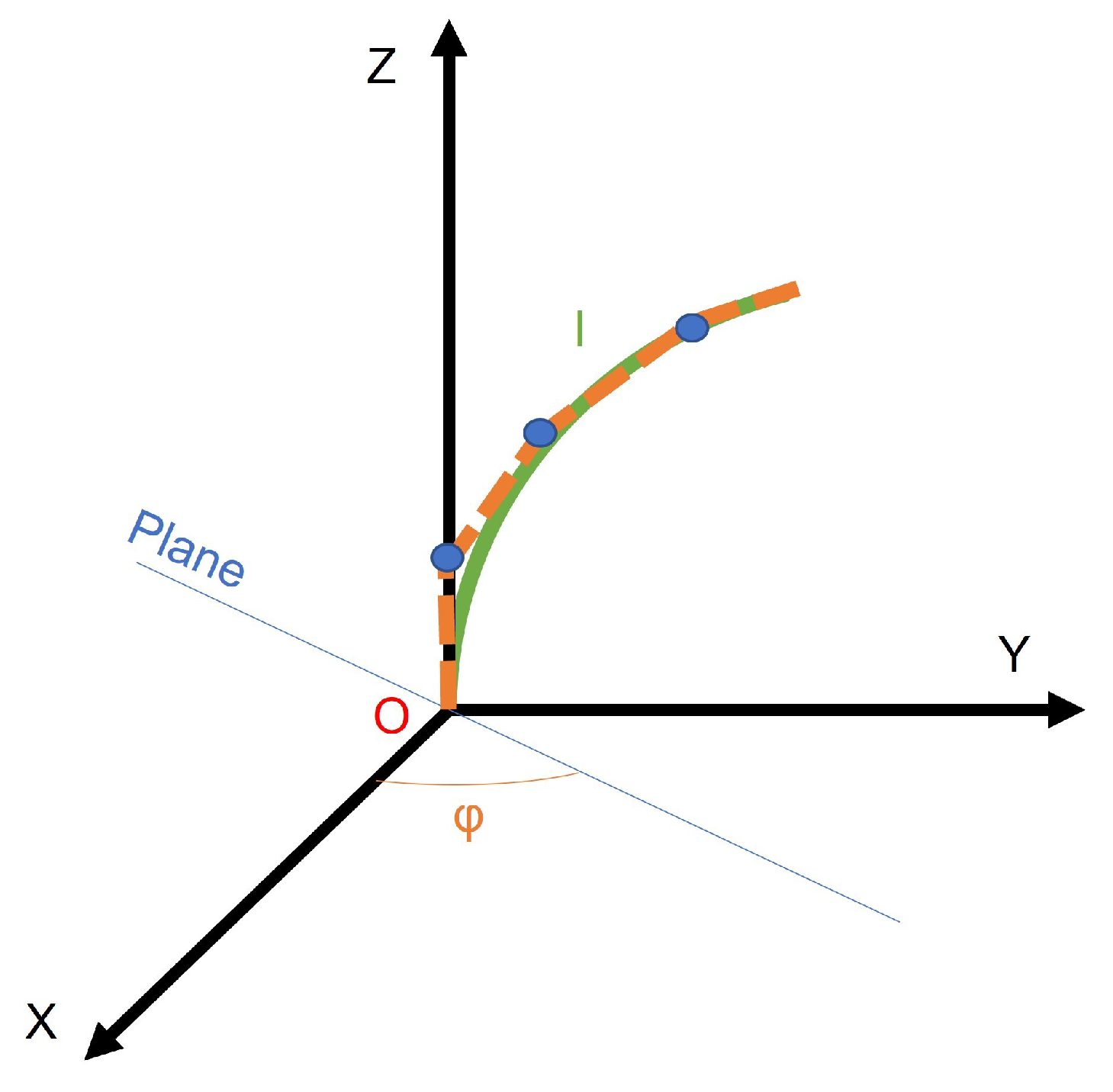
A 3-D arc can be defined in space, with the origin O of the reference system located in the centre of its inferior base (see Figure 8). The z axis is defined as orthogonal to such section, tangent to the curve of the arc. It would be desirable that the x axis is pointed to the centre of the arc, as in the $S_{rotate}$ reference frame in Figure 8, but this is not always possible in all instances. Therefore, to not lose generality, the x axis can be arbitrarily defined, as long as it is orthogonal to the z axis. The y axis is then obtained by the cross product, maintaining the requirements of orthogonality.

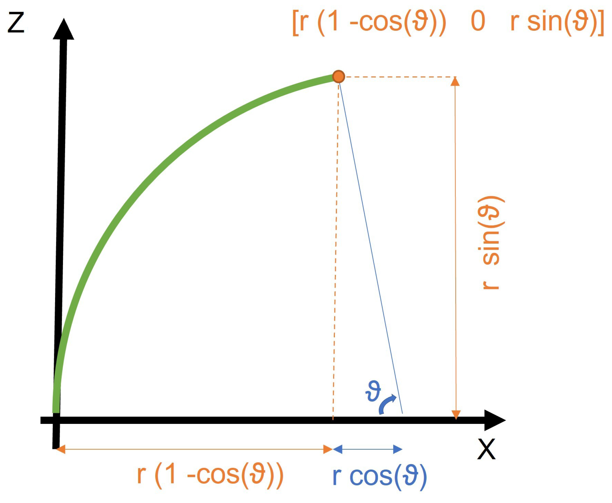
The arch itself uses geometric parameters: its length l, the curvature $\kappa$ (which is easily transformed into the angle $\theta$) and the orientation of the plane that contains the arch defined by the angle $\varphi$. The problem consists of obtaining the relationships between curvature parameters $\kappa ,\varphi$ and l and the endpoint of the arc $x_e,y_e$ and $z_e$.

This objective may be achieved by combining two movements (see Equation (4)): firstly, a rotation of $\varphi$ degrees around the Z axis can be applied, therefore obtaining the desired $S_{rotate}$ reference frame. Afterwards, the second transformation includes both a translation and a rotation alongside the arch. The translation sets the endpoint in the final point of the section, while the rotation leaves the Z axis tangent to the section and the X axis pointing to the centre of rotation.

$${}^{k-1}{A}_k=T_{rotate}\left(\varphi \right)·T_{2d\_arch}(\varphi ,\kappa ,l)$$

(4)

Obtaining $T_{rotate}\left(\varphi \right)$ is simple, since it is a rotation matrix around the z axis of ${\varphi }_k$ degrees:

$$T_{rotate}=\left[\begin{array}{cccc}cos\varphi & -sin\varphi & 0& 0\\ sin\varphi & cos\varphi & 0& 0\\ 0& 0& 1& 0\\ 0& 0& 0& 1\end{array}\right]$$

(5)

As far as the plane arch representation is concerned, a homogeneous transformation between two reference frames can be used. Following the arch means translating the origin of the transformed reference frame to its endpoint, while also rotating the axis so that z is kept parallel to the arch’s tangent and x points to its centre. In order to represent the whole arch, and not only its endpoint, a new variable s is defined: $s\in [0,l]$.

The arch contained in the plane has a radius that can be obtained from its curvature ($r=\frac{1}{\kappa }$), and the total angle it rotates around the positive axis y (see $\theta$ in Figure 9) would be defined as in Equation (6).

$$\theta =\kappa s$$

(6)

Using these two parameters, and seeing the geometry in Figure 9, the total translation could then be geometrically obtained:

$$t=\left[\begin{array}{ccc}r(1-cos\theta )& 0& rsin\theta \end{array}\right]=\left[\begin{array}{ccc}\frac{1-cos\kappa s}{\kappa }& 0& \frac{sin\kappa s}{\kappa }\end{array}\right]$$

(7)

Combining both the translation and the rotation in the same homogeneous transformation matrix:

$$T_{2d\_arch}=\left[\begin{array}{cccc}cos\kappa s& 0& sin\kappa s& \frac{1-cos\kappa s}{\kappa }\\ 0& 1& 0& 0\\ -sin\kappa s& 0& cos\kappa s& \frac{sin\kappa s}{\kappa }\\ 0& 0& 0& 1\end{array}\right]$$

(8)

The resulting kinematic equations are then given by multiplying matrices resulting from Equations (7) and (8), giving a general matrix ${}^{k-1}{A}_k$, that can be particularised at l:

$${}^{k-1}{A}_k\left(l\right)=\left[\begin{array}{cccc}cos\varphi cos\kappa l& -sin\varphi & cos{\varphi }_{k}sin\kappa l& \frac{cos\varphi (1-cos\kappa l)}{\kappa }\\ sin\varphi cos\kappa l& cos\varphi & sin\varphi sin\kappa l& \frac{sin\varphi (1-cos\kappa l)}{\kappa }\\ -sin\kappa l& 0& cos\kappa l& \frac{sin\kappa l}{\kappa }\\ 0& 0& 0& 1\end{array}\right]$$

(9)

4.1.2. Alternatives to Geometric Method

When assuming the PCC hypothesis, it is possible to apply the Denavit–Hartenberg method in order to obtain the equations, even though there are no discreet joints in the kinematic chain [7]. A recent example from the National University of Singapore has successfully used the Denavit–Hartenberg algorithm to estimate a flexible and continuous robot’s kinematic model actuated by cables [9]. In this work, MATLAB was used to calculate the mathematical equations through this method, demonstrating its efficiency and simplicity.

To do so, it is necessary to define a series of virtual joints that, altogether, allow to express the same mathematical model as the geometric method. Using these fictitious joints, it is possible to find a group of transformations following the rules of Denavit–Hartenberg which, through a finite number of parameters, represent the robotic section. As an example, several alternatives can be studied [5,7].

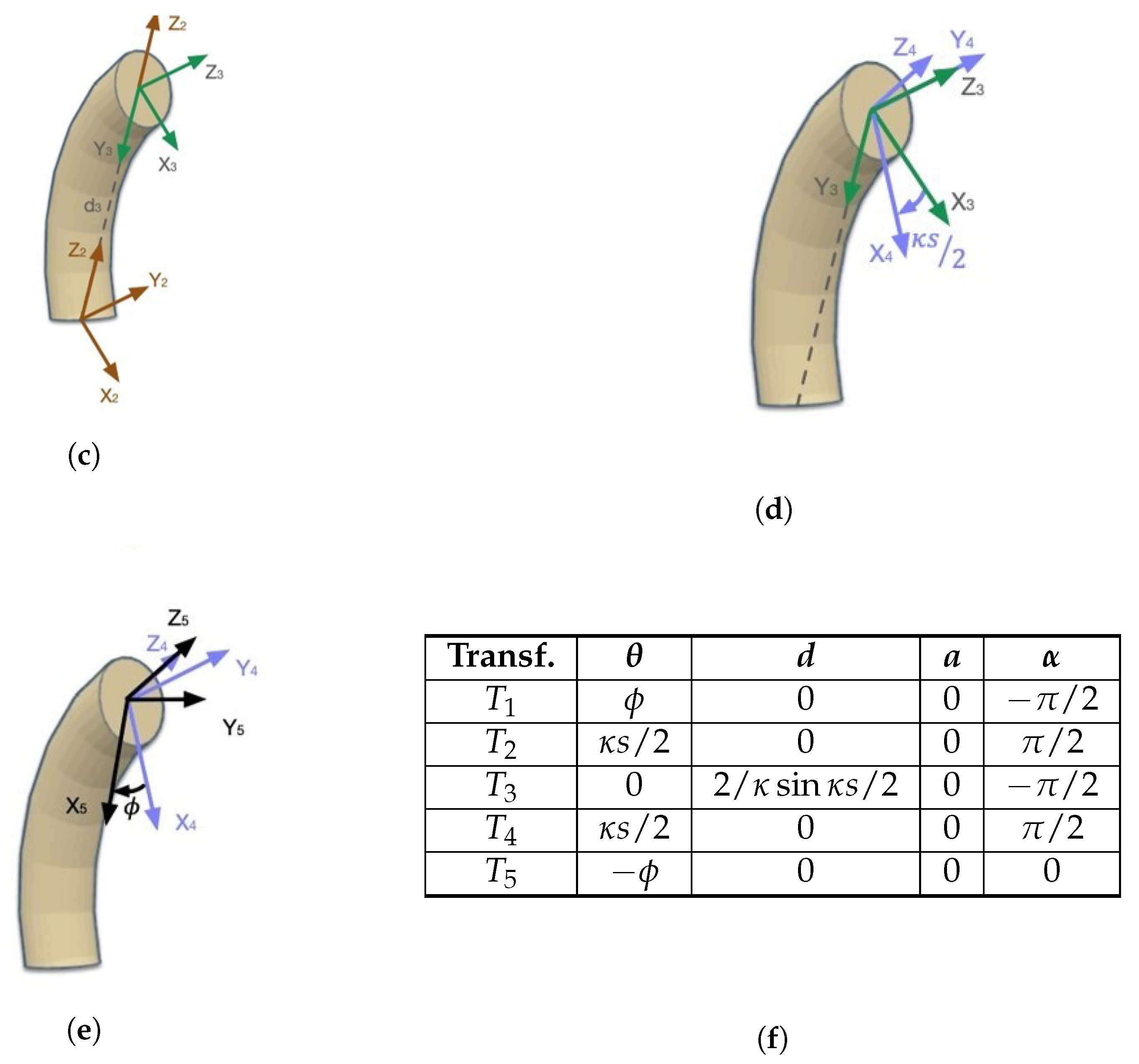
In order to show some continuity, and since this parameter definition allows the obtention of the same transformation as Equation (9), this section presents the Walker and Hannan proposal [31], modified by Webster [7] to match the previously stated reference systems. In it, five virtual joints are defined per section, which in Figure 10 are represented as different reference systems:

(1)

The first transformation is used to transform the problem in a two-dimensional curve, using the rotation $\varphi$.

(2)

The second transformation represents a rotation of ${\theta }_2=\frac{1}{2}\kappa s$ degrees, which is used to obtain a reference system pointing to the section’s endpoint.

(3)

The third transformation introduces the translation from the origin to the endpoint of the section curve $d_3=\frac{2}{\kappa }sin\frac{\kappa s}{2}$.

(4)

The fourth transformation rotates again ${\theta }_4=\frac{1}{2}\kappa s$ degrees to return the tangency to the curve in the endpoint.

(5)

Finally, the fifth transformation undoes the first transformation, returning to a three-dimensional problem.

Having defined these transformations, the Denavit–Hartenberg table can easily be filled, as seen in Figure 10f. Afterwards, the mathematical equations (the full transformation matrix) can be obtained by applying these parameters to the same method explained in Section 3.

In addition to this method, several additional algorithms can be used to obtain the same result: using differential geometry [19], Frenet’s curvature [7], the integral method [3], etc. In each of these methods, an equivalent matrix transformation would be obtained, as Webster’s article presents [7], which is why they can also be considered as PCC methods. Afterwards, the same relationship between cables and section curvature parameters as previously obtained must be added, in order to obtain a complete kinematic model.

This perfect equivalency between methods when obtaining the equations implies that choosing the deduction method is indifferent. The mathematical equations that conform the kinematic model are all valid, and the only difference when studying all these processes may be the reference systems. Therefore, it is possible to choose the most intuitive method for the designer.

4.1.3. Dependent Transformation

The other required transformation is the one dependent on the robot’s geometry, that is, the transformation from the cables’ length to the curvature parameters, which is particular for each robot. This means that a completely general method for any hyper-redundant continuous robot cannot be given. However, for some of the most frequent cases, such as three or four cables per section robots (a higher number would not allow additional DOF) symmetrically distributed around the section; the equations have already been thoroughly studied and obtained in various articles. For example, the three-cable section placed equidistant to the backbone (forming an equilateral triangle) can be obtained following [5]. In ref. [7], this is explained for three and four cables with a similar mathematical process.

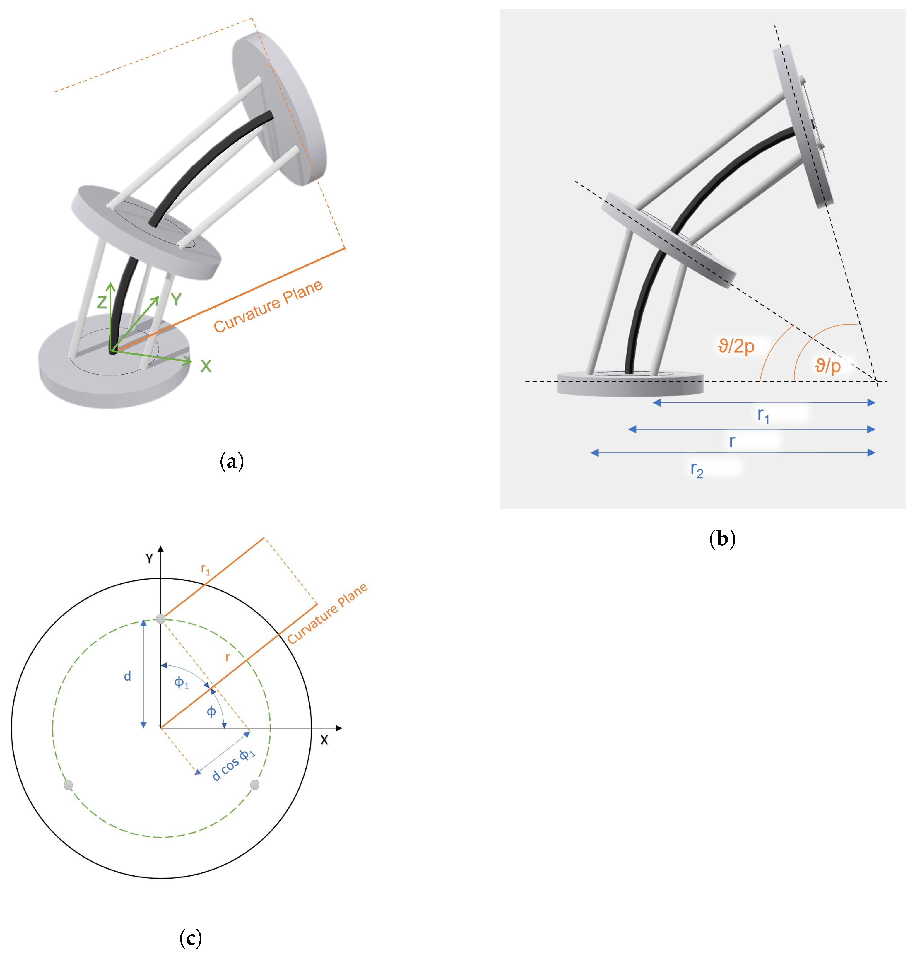
In this section, this last procedure is explained. Let us suppose a robot in which every section has three active cables, homogeneously and equidistantly distributed around the section’s centre, with a radius d (see Figure 11a). In that same robot’s section, several passive discs are used to guide the cables alongside the backbone (which follows the constant curvature hypothesis; therefore, the PCC model provides the position of each of the discs’ centres). These cables are modelled with the hypothesis that they join these passive discs with a straight line (see Figure 11b).

In Figure 11c, the projection in the plane of one of the section’s discs can be observed. In it, the curvature plane (which contains the circumference sector the backbone draws in space) can be seen, as well as the parallel plane that contains the curve that cable 1 follows (both in orange). If the three cables (grey) are equidistant to the section centre with a radius d, and homogeneously distributed, each of the cables i can be positioned by the angle ${\varphi }_i$. It can be easily deduced from the figure that:

$$r_i=r-dcos{\varphi }_i$$

(10)

The demonstration that these relationships are valid independently of the number of cables is simple, as long as the robot is compliant with the hypothesis of equidistant and homogeneous distribution.

Turning back to Figure 11b, the expressions for the hypothetical length of the section’s backbone ($l_c$) as well as the length of each of the cables $l_i$ can be derived; p being the number of passive discs in a section:

$$l_c=2·p·rsin(\theta /2p)$$

(11)

$$l_i=2·p·r_{i}sin(\theta /2p)$$

(12)

Multiplying Equation (10) by $2psin(\theta /2p)$, substituting in Equations (11) and (12), and solving it, the following expression is obtained:

$$l_c=l_i+d2p·sin(\theta /2p)·cos\left({\varphi }_i\right)$$

(13)

From this last expression, an important property can be deduced. Since cables are homogeneously distributed around the circumference, the total sum of angles ${\varphi }_i$ is zero. Using trigonometric relations, if Equation (13) is added for each of the cables, then the total length of the backbone could be calculated as the arithmetic average of the real cables’ lengths (independently of the number of cables that section has $f_k$).

$$l_c=\sum _{i=1}^{f_k}\frac{l_i}{f_k}$$

(14)

Going back to the three-cable example, applying Equation (13) to two cables and given that they must give the same $l_c$, then Equation (15) is obtained.

$$d2psin(\theta /2p)=(l_2-l_1)/(cos{\varphi }_1-cos{\varphi }_2)$$

(15)

This same step can be applied to cables two and three. Afterwards, joining together both expressions:

$$\varphi ={tan}^{-1}\left(\frac{\sqrt{3}(l_2+l_3-2l_1)}{3(l_2-l_3)}\right)$$

(16)

Finally, the curvature parameters are obtained through Equations (11) and (12) by which:

$$sin(\theta /2p)=l_c/2pr=l_i/2p{r}_i$$

(17)

Then, for each cable i:

$$r_i=\frac{l_i}{\kappa l_c}$$

(18)

If Equation (10) is applied, then:

$$\kappa =\frac{(l_c-l_i)}{l_{c}dcos\left({\varphi }_i\right)}$$

(19)

Given the reference that has previously been defined:

$$\kappa =\frac{l_2+l_3-2l_1}{(l_1+l_2+l_3)dsin\left(\varphi \right)}$$

(20)

An expression that calculates $\kappa$ using the problem’s data can be deduced if substituting $\varphi$ with Equation (16) and the trigonometric expression $sin\left({tan}^{-1}(y/x)\right)=y/\sqrt{x^2+y^2}$ is applied:

$$\kappa =\frac{2\sqrt{{l_1}^2+{l_2}^2+{l_3}^2-l_1{l}_2-l_1{l}_3-l_2{l}_3}}{d(l_1+l_2+l_3)}$$

(21)

To obtain the actual length of the curve (only the cable length has been calculated), applying the geometric definitions to Equation (11):

$$l=\frac{2p}{\kappa }{sin}^{-1}\left(\frac{l_c\kappa }{2p}\right)$$

(22)

Finally, applying Equations (21) and (14):

$$l=\frac{pd(l_1+l_2+l_3)}{2\sqrt{l_1^2+l_2^2+l_3^2-l_1{l}_2-l_1{l}_3-l_2{l}_3}}{sin}^{-1}\left(\frac{\sqrt{l_1^2+l_2^2+l_3^2-l_1{l}_2-l_1{l}_3-l_2{l}_3}}{3pd}\right)$$

(23)

Combining the two steps (cables → curvature parameters and curvature parameters → robot state), a direct kinematic model is completely defined for a hyper-redundant continuous robot with PCC hypothesis. If the expression for a multisection robot is desired, then the different transformations for the series of sections should be combined. Nevertheless, it must be taken into account that some corrections may be needed in these cases, since some sections may affect the others. Iterative algorithms [32] or optimisation may be used to improve the model [33].

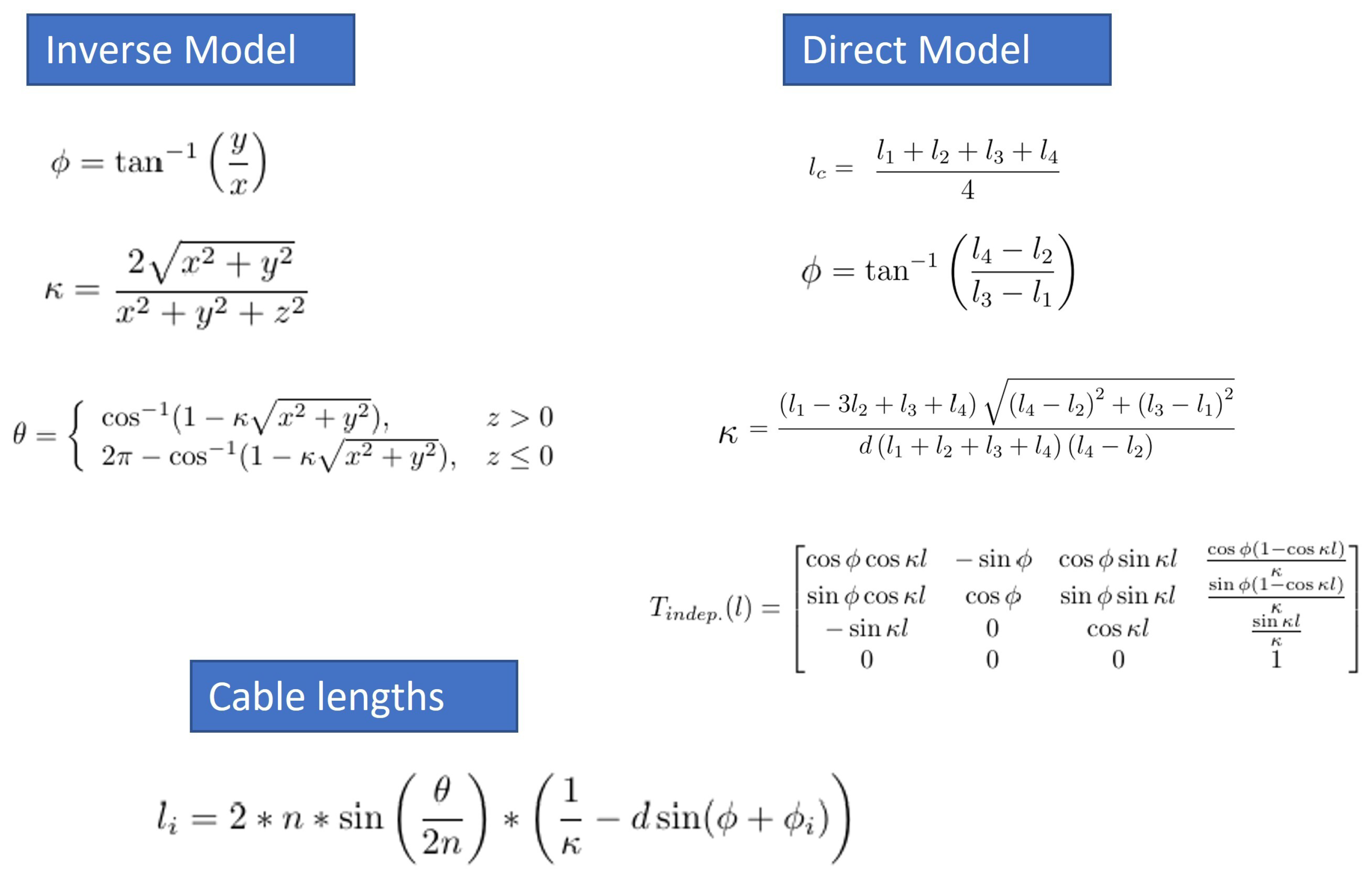
4.2. Inverse Kinematics

In this section, a possible approach to inverse kinematics is explained. The methodology assumes that the state for each section is already fixed (that is, the optimisation algorithm has already been applied). The objective when applying these equations is, therefore, once the sections have been positioned in space for a certain configuration, to obtain the geometric parameters and translate them to cable lengths that each section requires.

Mathematically this is translated as obtaining $l_1,l_2,\cdots ,l_f$ when introducing ${\left[\begin{array}{ccc}x& y& z\end{array}\right]}^t$ into the equations. The reason for using the Cartesian coordinates was discussed in Section 2.3: the PCC hypothesis describes the configuration of a section using three curvature parameters. Therefore, there are three degrees of freedom with which both the position and the orientation are perfectly defined. Choosing the Cartesian coordinates is an arbitrary decision, but the orientation could also be used (and the geometric transformations could be found analytically).

As in previous models, once the section state has been defined, two transformations are needed (see Figure 12). One of them is the geometric definition of the curvature parameters to extract them from the sections’ states. Afterwards, a robot-dependent transformation is needed, equivalent to that in direct kinematics. The relationship between curvature parameters and cable lengths is not general for all cases and must be examined individually.

Firstly, and given the assumption of the constant curvature hypothesis, it is necessary to obtain the curvature parameters given a certain endpoint ${\left[\begin{array}{ccc}x& y& z\end{array}\right]}^t$ for each robot section. Orientation is fixed when three parameters are given, as curvature parameters imply the robot only has three degrees of freedom per section. To do so, the method in [30] is followed. Beginning with the azimuthal angle $\varphi$, it can be obtained by a simple relationship:

$$\varphi ={tan}^{-1}\left(\frac{y}{x}\right)$$

(24)

Curvature is then obtained by analysing the robot’s arch in the vertical plane that contains it and searching for its radius (because $\kappa =1/r$). In this case, the endpoint of the section can be found in coordinates $x^{\prime }=\sqrt{x^2+y^2}$, $z^{\prime }=z$. Then, the radius can be equalled to the distance from the centre of the arch to its endpoint.

$${(\sqrt{x^2+y^2}-r)}^2+z^2=r^2$$

Finding r and inverting:

$$\kappa =\frac{2\sqrt{x^2+y^2}}{x^2+y^2+z^2}$$

(25)

Finally, to obtain the value of the arch’s length l, the $\theta$ angle must be used. Analysing again the arch contained in a plane, the following values can be extracted:

$$\theta =\left\{\begin{array}{cc}{cos}^{-1}(1-\kappa \sqrt{x^2+y^2}),\hfill & z>0\\ 2\pi -{cos}^{-1}(1-\kappa \sqrt{x^2+y^2}),\hfill & z\le 0\end{array}\right.$$

(26)

Lastly, the transformation to obtain l is purely geometrical: $l=r\theta$ = $\theta /\kappa$.

When obtaining an inverse kinematic model, it is essential to pay attention to the possible singularities such a model might have, which may cause further problems when trying to apply the equations. In this case, singularities for both $\kappa$ and $\varphi$ appear when the endpoint is located in the vertical axis [30]:

• $\varphi$: Vertical axis z corresponds to the set of points in which $x=0$ and $y=0$, so that in those cases when the robot’s endpoint is in the z axis, any value of $\varphi$ can be set.
• $\kappa$: In this case, two possibilities must be taken into account. Whenever $z\ne 0$, then $\kappa =0$ and $l=z$ can be used, as long as the robot’s length can be varied and z has a positive value (other cases should be studied individually). On the other hand, if $z=0$, then the robot’s endpoint should be located precisely in the origin, thus forming a perfect circle. There could be many mathematical solutions to do so, choosing, as an example, $\kappa =0$, $\varphi =0$ and $\theta =2\pi$. It should be noted, though, that this situation is, in most cases, mechanically impossible to reach.

After obtaining the curvature parameters of a section, the following step would be to obtain the cables’ length that are required to achieve such configuration. As said before, it is a robot-dependant transformation, so the following equations must not be taken as true for every robot. However, in order to complete the kinematic model, the three-cable robot is studied. To do so, it is enough to combine Equations (12) and (13), presented in Section 4.1, which defined the cables’ length. Doing so, it is obtained that:

$$l_i=2·p·r_{i}sin(\theta /2p)$$

(27)

In the bibliography, other approaches to obtain this equation can be found through a different geometric deduction, which can afterwards be transformed into this expression through the definition of $r_i$ [5]:

$$l_i=2·p·sin\left(\frac{\theta }{2p}\right)·\left(\frac{1}{\kappa }-dsin(\varphi +{\varphi }_i)\right)$$

(28)

Another aspect that should be taken into account when working with the inverse kinematic model is relative to multisection robots. The extension of these equations of the cables’ length can be made with those relationships, as long as the strict order of the sections is followed when calculating the cables’ lengths. This is due to the fact that, whenever a cable crosses a certain section, its length through it should also be obtained (as a passive cable) with such sections’ curvature parameters.

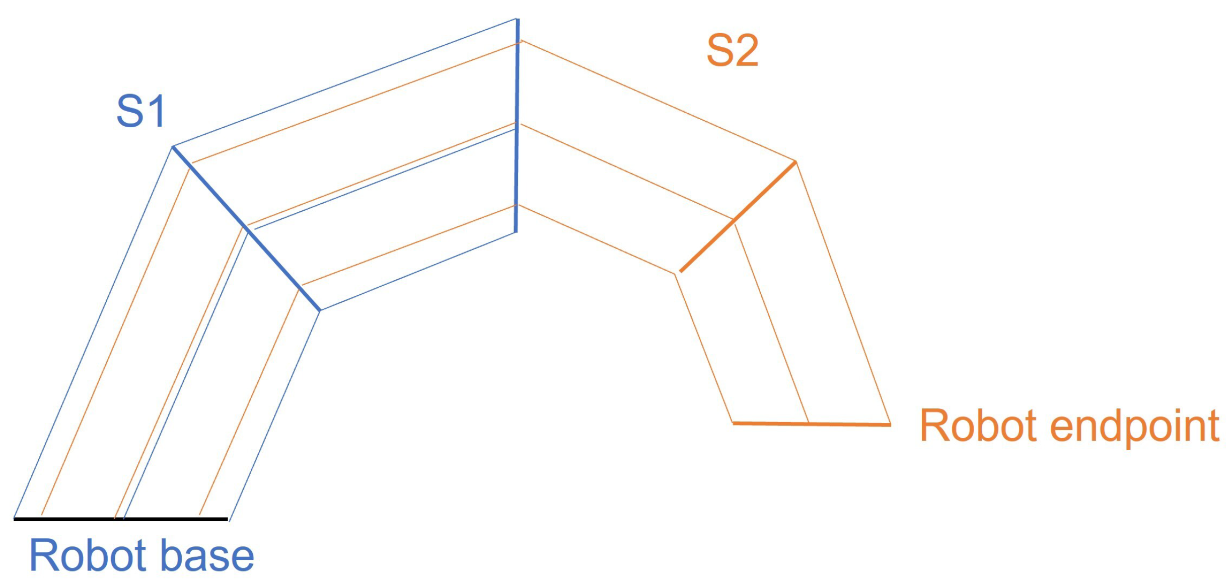
This is justified when looking at Figure 13. In it, a two-section robot is modelled. The second section $S2$ has a slightly reduced radius, while its cables have been rotated about those in section $S1$ to allow their simultaneity. Clearly, if the second section is to be positioned, in order to establish the cables’ length, both the segment of cable that is active in section $S2$ and the passive segment that goes through $S1$ should be taken into account.

As an example, for the robot in Figure 13, with $l_{ik}$ being the length of cable i for section k:

$$l_{i1}=2·p_1·sin\left(\frac{{\theta }_1}{2p_1}\right)·\left(\frac{1}{{\kappa }_1}-d_{1}sin(\varphi +{\varphi }_i)\right)$$

(29)

$$l_{i^{\prime }2}=2·p_1·sin\left(\frac{{\theta }_1}{2p_1}\right)·\left(\frac{1}{{\kappa }_1}-d_{1}sin(\varphi +{\varphi }_{i^{\prime }})\right)+2·p_2·sin\left(\frac{{\theta }_2}{2p_2}\right)·\left(\frac{1}{{\kappa }_2}-d_{2}sin(\varphi +{\varphi }_{i^{\prime }})\right)$$

(30)

In particular, the previous formulae should be applied thrice. Once to calculate the $S1$ cables’ length, directly as it was explained above (as a single-section robot). Then, and still using curvature parameters for $S1$ but changing d and ${\varphi }_i$, they should be applied again to the $S2$ cables. Finally, to that length, the values obtained by applying the formulae to an “isolated” $S2$ must be added.

Generalising for n sections, it can be easily verified that, in the first section of the robot, the formulae must be applied for each of the cables that manage the whole n sections. In the second section, they must be applied again to all but one section. Extrapolating this to all sections and assuming $f_k$ cables per section, the total number of operations that must be computed for n sections is:

$$f_k(n+(n-1)+\cdots +2+1)=f_k\sum _{j=1}^{n}j=f_k\frac{n(n+1)}{2}$$

It should be noted, though, that even if these equations have been obtained geometrically (and therefore should be applicable to any robot that follows the constant curvature hypothesis) they cannot be directly applied to all robots. Currently, much work is being put into variable-length robots, that is, that can grow larger or become smaller depending on the task being done. Other robots, such as soft continuous robots, can retract to diminish their length. In these cases, it may be possible to work with the inverse kinematics hereby presented but with some adjustments being made.

On the other hand, most current continuous robots have a rigid backbone, which implies that the length between sections must be practically constant. In these cases, it must be taken into account that the state space is not completely controllable. One of its degrees of freedom (the length between sections) is already fixed, and therefore the 3-D space is not completely reachable. As a result, these restrictions must be included in the kinematic equations for similar reasons to those explained in Section 2.2.

Finally, another effect should be considered. The coupling of sections may affect changes in shape in sections next to the base when trying to modify further segments of the robot. Although they may sometimes be neglected, a tangle/untangle algorithm designed by Jones and Walker may be used to improve accuracy [32].

4.3. Differential Kinematics

The differential model is the one that relates the velocities of the global reference system with those for each of the actionable degrees of freedom. That is, it would relate the change rate of the cables’ lengths to the velocities of the robot’s joints. It is an alternative to the direct kinematic model, as its integration would also give the position and orientation of the robot.

The obtention of a differential kinematic model can be achieved in two different ways. The first option could be deriving the direct kinematic model equations. However, it is frequently not desirable to use this method, as derivation is not computationally efficient. This could be solved with a similar method as the ones already explained, which separates the independent kinematics and those equations that explicitly depend on the robot being used.

Therefore, the most common solution is to derive separately the two transformations already described in Figure 7. This would lead to a specific expression of the relationship between the curvature’s parameters rate change and the section’s curvature parameter velocities, and another one between the curvature and the joints’ speeds.

There are several ways of obtaining the first Jacobian matrix. Some works, such as [31], do so by using the direct transformation matrices of the Denavit–Hartenberg method. The main problem with using traditional calculations (see [34]) for differential real-time kinematics is the extremely high number of operations they involve, especially when the reference points of the robot are constantly changing (due to its reconfigurable feature) [35]. The most common alternative approach uses screw theory to obtain a more computationally efficient representation [36].

However, in a work by Chembrammel and Kesavadas [35], a novel algorithm for calculating the Jacobian of a manipulator is proposed while applying it to a hyper-redundant robot. It is based on decomposing the Jacobian as the product of two matrices: L and P. Although it is directly applied to discreet robots, it can easily be adjusted to be useful in our PCC method. The article demonstrates the algorithm and applies it to a 2-DOF robot. In this work, the needed adaptation is explained.

In order to use the algorithm, the Kronecker product for matrices must be defined:

$$A\otimes B=\left[\begin{array}{ccc}{a}_{11}& \cdots & a_{1n}\\ \cdots & \cdots & \cdots \\ a_{m1}& \cdots & a_{mn}\end{array}\right]\otimes \left[\begin{array}{ccc}{b}_{11}& \cdots & b_{1n^{\prime }}\\ \cdots & \cdots & \cdots \\ b_{m^{\prime }1}& \cdots & b_{m^{\prime }{n}^{\prime }}\end{array}\right]=\left[\begin{array}{ccc}{a}_{11}B& \cdots & a_{1n}B\\ \cdots & \cdots & \cdots \\ a_{m1}B& \cdots & a_{mn}B\end{array}\right]=\left[\begin{array}{ccccccc}{a}_{11}{b}_{11}& \cdots & a_{11}{b}_{1n^{\prime }}& \cdots & a_{1n}{b}_{11}& \cdots & a_{1n}{b}_{1n^{\prime }}\\ \cdots & \cdots & \cdots & \cdots & \cdots & \cdots & \cdots \\ a_{11}{b}_{m^{\prime }1}& \cdots & a_{11}{b}_{m^{\prime }{n}^{\prime }}& \cdots & a_{1n}{b}_{m^{\prime }1}& \cdots & a_{1n}{b}_{m^{\prime }{n}^{\prime }}\\ \cdots & \cdots & \cdots & \cdots & \cdots & \cdots & \cdots \\ a_{m1}{b}_{11}& \cdots & a_{m1}{b}_{1n^{\prime }}& \cdots & a_{mn}{b}_{11}& \cdots & a_{mn}{b}_{1n^{\prime }}\\ \cdots & \cdots & \cdots & \cdots & \cdots & \cdots & \cdots \\ a_{m1}{b}_{m^{\prime }1}& \cdots & a_{m1}{b}_{m^{\prime }{n}^{\prime }}& \cdots & a_{mn}{b}_{m^{\prime }1}& \cdots & a_{mn}{b}_{m^{\prime }{n}^{\prime }}\end{array}\right]$$

(31)

To be more clear, $I_2$ being the identity of dimension 2 × 2 and A another 2 × 2 matrix:

$$I_2\otimes A=\left[\begin{array}{cccc}1·a_{11}& 1·a_{12}& 0·a_{11}& 0·a_{12}\\ 1·a_{21}& 1·a_{22}& 0·a_{21}& 0·a_{22}\\ 0·a_{11}& 0·a_{12}& 1·a_{11}& 0·a_{12}\\ 0·a_{21}& 0·a_{22}& 1·a_{21}& 0·a_{22}\end{array}\right]=\left[\begin{array}{cccc}{a}_{11}& a_{12}& 0& 0\\ a_{21}& a_{22}& 0& 0\\ 0& 0& a_{11}& a_{12}\\ 0& 0& a_{21}& a_{22}\end{array}\right]$$

(32)

Having defined the Kronecker product, to begin the algorithm, the transformation matrix from the base to the endpoint of the section is needed. It was calculated in Equation (9). The three variables that are used to calculate the differential equations are l, $\varphi$ and $\kappa$. Afterwards, the matrices $L_i$ are calculated using:

$$L_i=\frac{\partial T_{indep}\left(q\right)}{\partial q_i}$$

(33)

$q_i$ being the generalised coordinates already mentioned. The three matrices are:

$$L_l=\left[\begin{array}{cccc}-\kappa cos\varphi sin\kappa l& 0& \kappa cos\varphi cos\kappa l& cos\varphi sin\kappa l\\ -\kappa sin\varphi sin\kappa l& 0& \kappa sin\varphi cos\kappa l& sin\varphi cos\kappa l\\ -\kappa cos\kappa l& 0& -\kappa sin\kappa l& cos\kappa l\\ 0& 0& 0& 0\end{array}\right]$$

(34)

$$L_{\varphi }=\left[\begin{array}{cccc}-sin\varphi cos\kappa l& -cos\varphi & -sin\varphi sin\kappa l& \left(\right(cos\kappa l-1)sin\varphi )/\kappa \\ cos\varphi cos\kappa l& -sin\varphi & cos\varphi sin\kappa l& -\left(\right(cos\kappa l-1)cos\varphi )/\kappa \\ 0& 0& 0& 0\\ 0& 0& 0& 0\end{array}\right]$$

(35)

$$L_{\kappa }=\left[\begin{array}{cccc}-lcos\varphi sin\kappa l& 0& lcos\varphi sin\kappa l& (cos\varphi (cos\kappa l-1))/{\kappa }^2+lcos\varphi sin\kappa l/\kappa \\ -lsin\varphi sin\kappa l& 0& lsin\varphi sin\kappa l& (sin\varphi (cos\kappa l-1))/{\kappa }^2+lsin\varphi sin\kappa l/\kappa \\ -lcos\kappa l& 0& -lsin\kappa l& (lcos\kappa l)/\kappa -sin\kappa l/{\kappa }^2\\ 0& 0& 0& 0\end{array}\right]$$

(36)

Then, the matrix L is built by joining the three submatrices:

$$L=\left[\begin{array}{ccc}{L}_l& L_{\varphi }& L_{\kappa }\end{array}\right]$$

(37)

In the work by Chembrammel and Kesavadas [35], the algorithm is general for any point in the reference frame. In this case, the endpoint is used, defined as the origin vector when transformed by $T_{indep}$:

$$p={\left[\begin{array}{cccc}0& 0& 0& 1\end{array}\right]}^T$$

(38)

The algorithm proposed divides the Jacobian into two parts: the linear velocity Jacobian and the angular velocity Jacobian. To start with the linear part, the matrix $P_{linear}$ is obtained using the Kronecker product with the identity:

$$P_{lin}=I_3·p={\left[\begin{array}{cccccccccccc}0& 0& 0& 1& 0& 0& 0& 0& 0& 0& 0& 0\\ 0& 0& 0& 0& 0& 0& 0& 1& 0& 0& 0& 0\\ 0& 0& 0& 0& 0& 0& 0& 0& 0& 0& 0& 1\end{array}\right]}^T$$

(39)

For the angular part, another $P_{ang}$ must be obtained as the inverse of the original transformation matrix (or $T_{indep}$). Finally, each of the Jacobians (both linear and angular) can be found by multiplying both matrices for each part:

$$J_{lin}=L{P}_{lin}=\left[\begin{array}{ccc}cos\varphi sin\kappa l& (sin\varphi (cos\kappa l-1\left)\right)/\kappa & (cos\varphi (cos\kappa l-1))/{\kappa }^2+lcos\varphi sin\kappa l/\kappa \\ sin\varphi sin\kappa l& -(cos\varphi (cos\kappa l-1\left)\right)/\kappa & (sin\varphi (cos\kappa l-1))/{\kappa }^2+lsin\varphi sin\kappa l/\kappa \\ cos\kappa l& 0& (lcos\kappa l)/\kappa -sin\kappa l/{\kappa }^2\end{array}\right]$$

(40)

The angular Jacobian is obtained somewhat differently. For each generalised coordinate $q_i$, the product $L_{i}P$ is calculated. For each coordinate, a different component of the product $L_{i}P$ is obtained:

$$J_{\omega }=\left[\begin{array}{ccc}{\left(L_{1}P\right)}_{(3,2)}& {\left(L_{2}P\right)}_{(3,2)}& {\left(L_{3}P\right)}_{(3,2)}\\ {\left(L_{1}P\right)}_{(1,3)}& {\left(L_{2}P\right)}_{(1,3)}& {\left(L_{3}P\right)}_{(1,3)}\\ {\left(L_{1}P\right)}_{(2,1)}& {\left(L_{2}P\right)}_{(2,1)}& {\left(L_{3}P\right)}_{(2,1)}\end{array}\right]=\left[\begin{array}{ccc}-\kappa sin\varphi & 0& -lsin\varphi \\ \kappa cos\varphi & 0& lcos\varphi \\ 0& 1& 0\end{array}\right]$$

(41)

With this, the conventional Jacobian could be obtained by combining the two matrices in one:

$$J=\left[\begin{array}{c}{J}_{lin}\\ J_{\omega }\end{array}\right]$$

(42)

This represents the differential model for the curvature parameters, that is, the independent part of the robot. The work by Chembrammel and Kesavadas [35] also uses further expressions to calculate the derivative of the Jacobian, allowing for numeric integration over time. These expressions are not particularised for the example that was developed here but can be easily calculated:

$$\dot{L}=\frac{\partial L}{\partial q_i}$$

(43)

$$\dot{J_{lin}}=\sum _{i=1}^n\frac{\partial J_{lin}}{\partial q_i}\dot{q_i}=\sum _{i=1}^n\frac{\partial L}{\partial q_i}P\dot{q_i}$$

(44)

$$\dot{J_{\omega }}=\sum _{i=1}^n\frac{\partial J_{\omega }}{\partial q_i}\dot{q_i}$$

(45)

$$\frac{\partial J_{\omega ,i}}{\partial q_j}{\left(\left[\begin{array}{ccc}{\left(L_{i}P\right)}_{(3,2)}& {\left(L_{i}P\right)}_{(1,3)}& {\left(L_{i}P\right)}_{(2,1)}\end{array}\right]\right)}^T$$

(46)

$$\frac{\partial L_{i}P}{q_j}=\left(\frac{\partial L_i}{\partial q_j}-L_i{T}_{indep}^{-1}{L}_j\right)T_{indep}^{-1}$$

(47)

As said, this would be a partial differential model: it would only take into account the independent part of the robot, and thus it is completely general for any PCC-compliant robot. However, this method for obtaining Jacobians would also be plausible using the complete equations. The only necessary steps would be substituting the relationships between cables and curvature parameters (such as Equations (21) and (16)) in the transformation matrix (Equation (9)). Then, the process would be repeated using $l_1,l_2,\cdots ,l_n$ as generalised coordinates. This would return a complete differential model.

5. LSK—Linearised Segment Kinematics

PCC kinematics presents some problems when applied to certain applications. One of them is the great computational cost it represents when enlarging the number of sections of a robot, due to the number of operations already seen in the inverse kinematics. This means that using it for real-time applications in robots might not be enough, so work is being conducted to find alternative methods that evade these limitations. One example is Linearised Segment Kinematics, which also eliminates the PCC singularities [37].

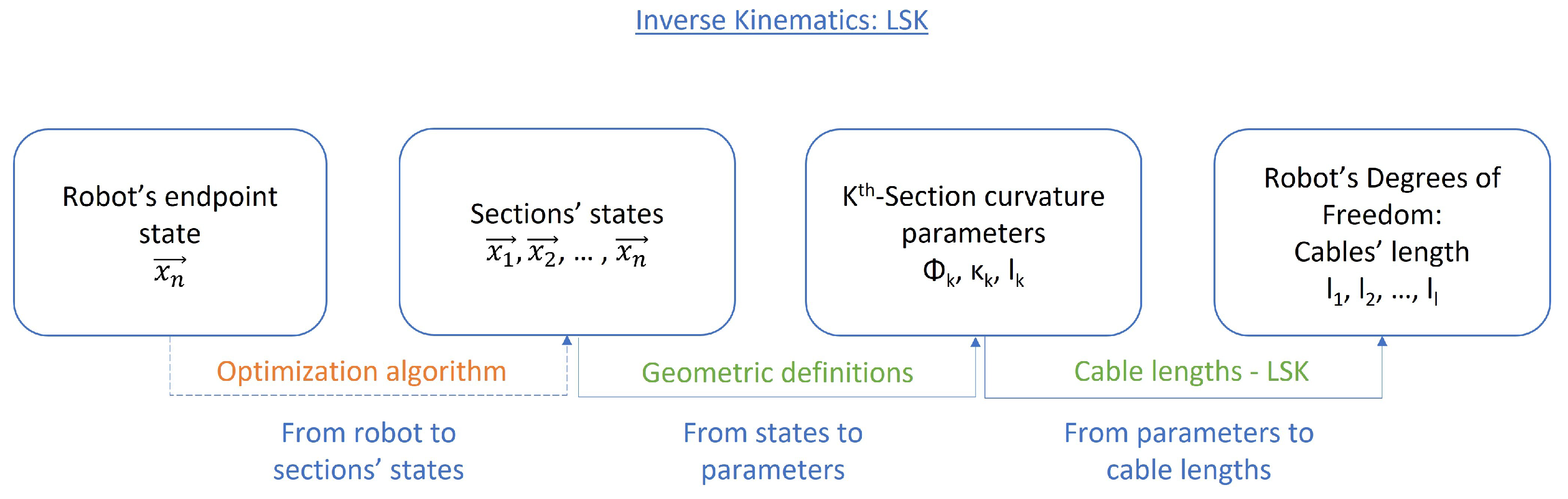
As a derived method from the PCC, its general diagram is quite similar (see Figure 14). The main change the LSK method provides is the linearisation equations for cable lengths. It is indeed a dependent method on the geometry of the robot. However, the fact that many of the hyper-redundant robots are quite similar in their functional morphology makes it easy to find linearised equations for many robots. Only the inverse kinematics figure is shown, but linearised equations for cable lengths can be applied both to direct and inverse kinematics.

This method is based on linearising the kinematic equations for each cable, simplifying the equations of each section, and therefore, the robot’s kinematic model. To do so, an adapted expression of the PCC formulae is used, combining Equations (10) and (13) and applying trigonometric relationships:

$$l_i=2·sin\left(\frac{\theta }{2p}\right)·\left(\frac{l_{c}p}{\theta }-r_{c}sin(\varphi +{\varphi }_i)\right)$$

(48)

To avoid the computational cost of calculating sines, to eliminate the dividing by zero ($\theta =0$) singularity, and in order to reduce the number of necessary iterations when the number of sections increases, linearisation can be applied to this equation.

In the work presented in [37], whether this linearisation is necessary or not is firstly justified. To do so, it begins by calculating the neutral fibre of the robot, which becomes an example for further calculations:

$$l\ge 2·sin\left(\frac{\theta }{2p}\right)·\left(\frac{l_{c}p}{\theta }-r_{c}sin\left(\varphi \right)\right)$$

Cables are considered to work with tensile stress and do not offer resistance to compression. This way, any point that requires less cable length could be potentially reached, which forces the apparition of an inequality. Afterwards, the Maclaurin series for $\theta$ is applied (Taylor series when $\theta =0$), and as a result:

$$l\approx l^{\prime }\ge l_c-r_c\frac{\theta }{p}$$

(49)

If linearisation were to be applied to the whole range of possible angles of the robot, it could be verified that linearising for a certain point (such as the origin), in those points excessively far apart from those points, would present excessive errors in the equations. However, assuming several segments exist in a single section (passive discs), this total turning angle is divided among them, therefore reducing the subsequent error, which becomes acceptable. From this perspective, Barrientos and Dong demonstrate that the maximum error this development shows is $0.7\%$.

Linearising the equations for each cable $l_i$ and applying the Maclaurin series again, the following relationship appears:

$$l_i^{\prime }\ge -p·r_c·\theta ·(cos\left({\varphi }_i\right)·cos\left(\varphi \right)+sin\left({\varphi }_i\right)·sin\left(\varphi \right))+l_c$$

(50)

Since what is actually needed is the increment of cable length with reference to a neutral position, the constant can be eliminated, thus expressing the equation as a difference of lengths. Apart from that, it can be observed that the system is left as a product between a certain scale factor $K\left(\theta \right)$, a matrix that only depends on the robot geometry $\mathbf{A}\left({\varphi }_i\right)$ and the trigonometric variables that use $\varphi$:

$$\left[\begin{array}{c}\Delta l_1\\ \Delta l_2\\ \cdots \\ \Delta l_f\end{array}\right]⪆K\left(\theta \right)\mathbf{A}\left({\varphi }_i\right)\left[\begin{array}{c}cos\left({\varphi }_i\right)\\ sin\left({\varphi }_i\right)\end{array}\right]=-r_c\theta \left[\begin{array}{cc}cos\left({\varphi }_1\right)& sin\left({\varphi }_1\right)\\ cos\left({\varphi }_2\right)& sin\left({\varphi }_2\right)\\ \cdots & \cdots \\ cos\left({\varphi }_{np}\right)& sin\left({\varphi }_{np}\right)\end{array}\right]\left[\begin{array}{c}cos\left({\varphi }_i\right)\\ sin\left({\varphi }_i\right)\end{array}\right]$$

(51)

This would then represent the inverse kinematic model for a single section. To obtain the direct kinematics, as long as the length increments are coherent, it could be inferred that:

$$\left[\begin{array}{c}cos\left({\varphi }_i\right)\\ sin\left({\varphi }_i\right)\end{array}\right]⪅-\frac{1}{r_c\theta }{\left[\begin{array}{cc}cos\left({\varphi }_1\right)& sin\left({\varphi }_1\right)\\ cos\left({\varphi }_2\right)& sin\left({\varphi }_2\right)\\ \cdots & \cdots \\ cos\left({\varphi }_{np}\right)& sin\left({\varphi }_{np}\right)\end{array}\right]}^T\left[\begin{array}{c}\Delta l_1\\ \Delta l_2\\ \cdots \\ \Delta l_f\end{array}\right]$$

(52)

6. Kinetic Robot Modelling Using Elastic Properties

Modelling hyper-redundant robots without the constant curvature hypothesis is mostly performed by kinetic modelling techniques, using elasticity parameters and taking the different strains that apply to the robot system into account [15]. They are more precise but more complex models, and solving them requires more computational power.

One of the reasons why the PCC hypothesis might not always be accurate enough to represent a certain robot can be if its specific weight is too high. When it has a continuous backbone of a certain material, including its dynamic properties in the model might provide more accuracy to the results of the kinematic model.

In particular, two models are briefly described in this section. The equations are not derived as thoroughly as the previous models, although the cited articles contain the detailed procedure. The main difference between the two models is the continuity of the backbone properties: the first model (Pseudorigid Body—PRB) uses lumped parameters [15] (they are a finite set of parameters) while the second model (Cosserat Rod Theory—CRT) requires an infinite number of parameters to characterise it.

6.1. Pseudorigid Body

The Pseudorigid Body is a model that allows the calculation of large deflections in beams through modelling them as combination of rotation joints and springs. In particular, the most used model for backbones in hyper-redundant robots is the one proposed by Su in 2009 [38] (see Figure 15). It proposes using four rigid and straight segments (in orange) joined by three pin joints with three torsion springs (in blue) to model the portion of the robot between two consecutive discs (in green). It should be noted that, being a kinetic model, it uses forces instead of lengths as an input parameter (see Figure 16). Moreover, as it characterises the backbone’s dynamic parameters, it is oriented to robots with a continuous backbone of a homogeneous material.

The PRB proposes using four parameters optimised by Chen in [39]: ${\gamma }_0=0.125$, ${\gamma }_1=0.35$, ${\gamma }_2=0.388$ and ${\gamma }_3=0.136$ as the ratio of each of the four segments to the total length of the section. Now, if the angle ${\theta }_{k,i}$ is the angle of link i in section k, the transformation matrix in the plane of section k becomes:

$$T_{k,i}=\left[\begin{array}{cccc}cos\left({\theta }_{k,i}\right)& 0& sin\left({\theta }_{k,i}\right)& {\gamma }_{k,i}{l}_{j}sin\left({\theta }_{k,i}\right)\\ 0& 1& 0& 0\\ -sin\left({\theta }_{k,i}\right)& 0& cos\left({\theta }_{k,i}\right)& {\gamma }_{k_i}{l}_{j}cos\left({\theta }_{k,i}\right)\\ 0& 0& 0& 1\end{array}\right]$$

(53)

The section is finally modelled as the combination of the rotation to the plane (a rotation around z, $R_z$), the successive links and the rotation to undo the first turn. One final turn is added to represent a possible twist:

$${}^k{A}_{k+1}=R_z\left({\varphi }_j\right)T_{k,0}{T}_{k,1}{T}_{k,2}{T}_{k,3}{R}_z(-{\varphi }_j)R_z\left(ϵ\right)$$

(54)

Several aspects should be taken into account at this point. When Huang et al. proposed this model, they only considered one-segment robots without external forces [40]. However, Rao et al. proposed a modified model which contains these possibilities too, and as such, it is the one developed [15].

First of all, and using as input the tension ${\tau }_{j,i}$ of the cables over disc i, the force of cable j over the last disk n is calculated, using the vector $\overrightarrow{P_{j,n}{P}_{j,n-1}}$ between the origin of the cable at two consecutive discs:

$${\overrightarrow{F}}_{j,n}={\tau }_{j,n}\frac{\overrightarrow{P_{j,n}{P}_{j,n-1}}}{\left|\right|\overrightarrow{P_{j,n}{P}_{j,n-1}}\left|\right|}$$

(55)

For other disks i, the equation ends up as:

$${\overrightarrow{F}}_{j,i}={\tau }_{j,i}\frac{\overrightarrow{P_{j,i}{P}_{j,i-1}}}{\left|\right|\overrightarrow{P_{j,i}{P}_{j,i-1}}\left|\right|}+{\tau }_{j,i+1}\frac{\overrightarrow{P_{j,i+1}{P}_{j,i}}}{\left|\right|\overrightarrow{P_{j,i+1}{P}_{j,i}}\left|\right|}$$

(56)

The total force over a certain disc is then obtained when adding up external forces (typically on the tip of the robot, therefore accounted in the last disk), n being the last disk, i a generic disc and f the total number of cables:

$${\overrightarrow{F}}_n^T=\sum _{j=1}^f{\overrightarrow{F}}_{j,n}+{\overrightarrow{F}}_{ext}$$

(57)

$${\overrightarrow{F}}_i^T=\sum _{j=1}^f{\overrightarrow{F}}_{j,i}+{\overrightarrow{F}}_{i+1}i<n$$

(58)

From this, the involved moments are derived. Naming $\overrightarrow{O_i{O}_{q,i}}$ as the vector that joins the base of the disk i and the theoretical joint q, $\overrightarrow{M_{i,q}}$ as the total moment applied to disk i by joint q and $\overrightarrow{M_{j,i}^c}$ the tension that cable j applies to disk i:

$${\overrightarrow{M}}_{n,q}=\sum _{j=1}^f\overrightarrow{M_{n,j}^c}+\overrightarrow{O_n{O}_{q,n}}\times {\overrightarrow{F}}_n^T$$

(59)

$${\overrightarrow{M}}_{i,q}=\sum _{j=1}^f\overrightarrow{M_{i,j}^c}+\overrightarrow{O_i{O}_{q,i}}\times {\overrightarrow{F}}_i^T+{\overrightarrow{M}}_{i+1,q}i<n$$

(60)

The total moment for the section $\overrightarrow{M_i^T}$ is calculated as:

$${\overrightarrow{M}}_n^T=\sum _{j=1}^f\overrightarrow{M_{n,j}}+\overrightarrow{O_{n-1}{O}_n}\times {\overrightarrow{F}}_n^T$$

(61)

$${\overrightarrow{M}}_i^T=\sum _{j=1}^f\overrightarrow{M_{i,j}}+\overrightarrow{O_{i-1}{O}_i}\times {\overrightarrow{F}}_i^T+{\overrightarrow{M}}_{i+1}^{T}i<n$$

(62)

Taking this vector, the angle $\varphi$ can be calculated by knowing that the vector $\overrightarrow{y_i}$, perpendicular to the plane, is colinear with $\overrightarrow{M_i^T}-\overrightarrow{M_j^T}·\overrightarrow{z_i}$. Once this angle has been calculated, only the joints’ angles are missing to have a complete set of equations. To obtain these angles, the relationship used is:

$$\left|\right|\overrightarrow{M_i^T}-\overrightarrow{M_i^T}·\overrightarrow{z_i}\left|\right|=K_{{\Theta }_q}\frac{EI}{l_i}{\theta }_q$$

(63)

$EI$ being the characterising parameters for the material, l the length of the section and $K_{{\Theta }_q}$ certain parameters that were also optimised as: $K_{{\Theta }_1}=3.25$, $K_{{\Theta }_2}=2.84$ and $K_{{\Theta }_3}=2.95$ [39]. The last equation needed is used to obtain the twist parameter $ϵ$:

$$GJ{ϵ}_i=l_i{(}^{i-1}{T}_i{\overrightarrow{M}}_i){\overrightarrow{z}}_B$$

(64)

There is a great complexity to solve these equations. There are five independent kinematic variables per section (${\theta }_{1,i},{\theta }_{2,i},{\theta }_{3,i},{\varphi }_i$ and ${ϵ}_i$) and three independent dynamic variables per section ($M_{x,i}^T,M_{y,i}^T$ and $M_{z-i}^T$). There are also eight equations available per section (three equations in (62) where all the other terms are kinematic-dependent or known, three equations in (63) for the three joints, one equation for the colinearity condition and one equation in (64)). However, all sections must be solved at once due to the interdependence of sections, and it is a highly nonlinear system. Therefore, numerical methods must be used [41].

6.2. Cosserat Rod Theory

The Cosserat theory for elastic rods (CRT) is one of the most common techniques to model continuous beams and can be used to establish the backbone. This theory assigns six degrees of freedom to each point of the robot’s backbone while establishing some boundary conditions it must meet using kinetic equations [42]. This technique has been applied to several kinematic problems, each for a different robot configuration [24,43,44]. All these works present slightly different proposals, with the integration information needed to solve the problem.

In particular, the Cosserat Theory provides the relationship between the forces (or strains) applied to the robot and the position of the backbone at each of its points. Once again, taking into account this is a kinetic model, the inputs for the model are the strains suffered by the robotic arm. In particular, the development used by Jones [43] is presented below.

Using the definitions seen in Figure 17, the position and orientation of section i are defined by a position vector $\overrightarrow{p}\left(i\right)$ and a rotation matrix ${}^{i-1}{A}_i$. If we define $\overrightarrow{v}\left(i\right)$ as the linear velocity of an infinitesimal section from the rigid body, expressed in body coordinates, and $\overrightarrow{u}\left(i\right)$ as the infinitesimal rotation of the frame ${}^{i-1}{A}_i$, then the derivatives take the form:

$$\dot{\overrightarrow{p}}{=}^{i-1}{A}_i·\overrightarrow{v}$$

(65)

$$\dot{{}^{i-1}{A}_i}{=}^{i-1}{A}_i·\left[\begin{array}{ccc}0& -u_z& u_y\\ u_z& 0& -u_x\\ -u_y& u_x& 0\end{array}\right]$$

(66)

Now, six more variables are introduced: ${\overrightarrow{v}}^{*}$ and ${\overrightarrow{u}}^{*}$ represent the linear and angular velocity of the default (nondeformed) state of the rod; $\overrightarrow{m}\left(i\right)$ and $\overrightarrow{n}\left(i\right)$ represent the internal moment and force vectors, respectively; $\overrightarrow{f}$ is the applied force distribution; and $\overrightarrow{l}$ is the distributed moment. Then, applying equilibrium and using $\overrightarrow{m}\left(i\right)$ and $\overrightarrow{n}\left(i\right)$ as state variables:

$$\dot{\overrightarrow{n}}=-\overrightarrow{f}$$

(67)

$$\dot{\overrightarrow{m}}=-\overrightarrow{p}\times \overrightarrow{n}-\overrightarrow{l}$$

(68)

Finally, we need to introduce the material characterisation:

$$K_{se}\left(i\right)=\left[\begin{array}{ccc}GA\left(i\right)& 0& 0\\ 0& GA\left(i\right)& 0\\ 0& 0& EA\left(i\right)\end{array}\right]K_{bt}\left(i\right)=\left[\begin{array}{ccc}E{I}_{xx}\left(i\right)& 0& 0\\ 0& E{I}_{yy}\left(i\right)& 0\\ 0& 0& E{I}_{zz}\left(i\right)\end{array}\right]$$

(69)

To obtain a complete model, these matrices are introduced by the Constitutive Laws:

$$\overrightarrow{v}=K_{se}^{-1}{}^{i-1}{A}_i^T\overrightarrow{n}+{\overrightarrow{v}}^{*}$$

(70)

$$\overrightarrow{u}=K_{bt}^{-1}{}^{i-1}{A}_i^T\overrightarrow{m}+{\overrightarrow{u}}^{*}$$

(71)

Cosserat Theory per se is composed of Equations (65)–(68), (70) and (71). However, the theory of tendons and cables can also be coupled, taking into account that both the forces and the moments have an external (${\overrightarrow{f}}_e$, ${\overrightarrow{l}}_e$) and a tendon-caused (${\overrightarrow{f}}_t$, ${\overrightarrow{l}}_t$) component [44]. For brevity, the whole development is not added here, but tendon forces and moments are derived in the article from the tension of each cable ${\tau }_j$. For the solution, the operator $\widehat{w}$ is introduced as:

$$\widehat{\overrightarrow{w}}=\left[\begin{array}{ccc}0& -w_z& w_y\\ w_z& 0& -w_x\\ -w_y& w_x& 0\end{array}\right]$$

(72)

With this tool, and defining ${\overrightarrow{r}}_j$ as the vector from the origin of the attached frame to the tendon’s origin, the equations that relate forces to tendons can be found below (do not confuse scalar f, the total number of cables with vectorial $\overrightarrow{f}$, which are forces):

$${\overrightarrow{f}}_t=-\sum _{j=1}^f{\tau }_j\frac{{\widehat{\dot{\overrightarrow{p}}}}_j^2}{\left|\right|{\dot{\overrightarrow{p}}}_j{\left|\right|}^3}{\ddot{\overrightarrow{p}}}_j$$

(73)

$${\overrightarrow{l}}_t=-\sum _{j=1}^f{\tau }_i{(}^{i-1}{A}_i{\overrightarrow{r}}_j)\frac{{\widehat{\dot{\overrightarrow{p}}}}_j^2}{\left|\right|{\dot{\overrightarrow{p}}}_j{\left|\right|}^3}{\ddot{\overrightarrow{p}}}_j$$

(74)

These equations use the derivatives, which can be expressed in terms of kinematic variables:

$${\dot{\overrightarrow{p}}}_j{=}^{i-1}{A}_i(\widehat{\overrightarrow{u}}{\overrightarrow{r}}_j+{\dot{\overrightarrow{r}}}_j+\overrightarrow{v})$$

(75)

$${\ddot{\overrightarrow{p}}}_j{=}^{i-1}{A}_i(\widehat{\overrightarrow{u}}(\widehat{\overrightarrow{u}}{\overrightarrow{r}}_j+{\dot{\overrightarrow{r}}}_j+\overrightarrow{v})+\widehat{\dot{\overrightarrow{u}}}{\overrightarrow{r}}_j+\widehat{\overrightarrow{u}}{\dot{\overrightarrow{r}}}_j+{\ddot{\overrightarrow{r}}}_j+\dot{\overrightarrow{v}})$$

(76)

This would constitute an implicit set of equations for hyper-redundant robots with tendons. The article goes on to develop the expression in order to give an explicit state system. However, the idea of the CRT is clear in this excerpt, including the complexity of the model compared with the previous ones and the need to explicitly know the continuous expressions of forces and moments.

7. Optimization Algorithm—CCD and Natural CCD Algorithms

In previous sections, different models and hypotheses to simplify hyper-redundant robot modelling were described in detail. They form the basis for choosing the right equations for every robot. However, as seen in the general stages of kinematic hyper-redundant modelling, there are two steps that are completely general to all methods. One of them is the matrix multiplication for combining all the HTMs involved and has no further difficulty. Apart from that, an optimisation method is required to place each of the robot’s sections in space, in order to reach a certain endpoint.

So, as to have completeness in the kinematic models, a particular algorithm is proposed here as a possible solution to the problem. Of course, there are many alternative methods (numeric methods, neural networks, genetic algorithms or the pseudoinverse Jacobian). However, the algorithm of Natural CCD aims to obtain a computationally efficient solution, with high precision, that may be used in a Real-Time System (RTS) [26] and seems to fit in the proposed methodology (see Figure 18).

The CCD algorithm, which means Cyclic Coordinate Descent, is a method that, without using derivatives, finds a local minimum for a function. It is based on the concept that when minimising using generalised coordinates one by one on each iteration, the whole function is minimised in the end [25]. Applying this to inverse kinematics, the function to minimise is the euclidean distance between the robot’s endpoint and the desired destination or objective.

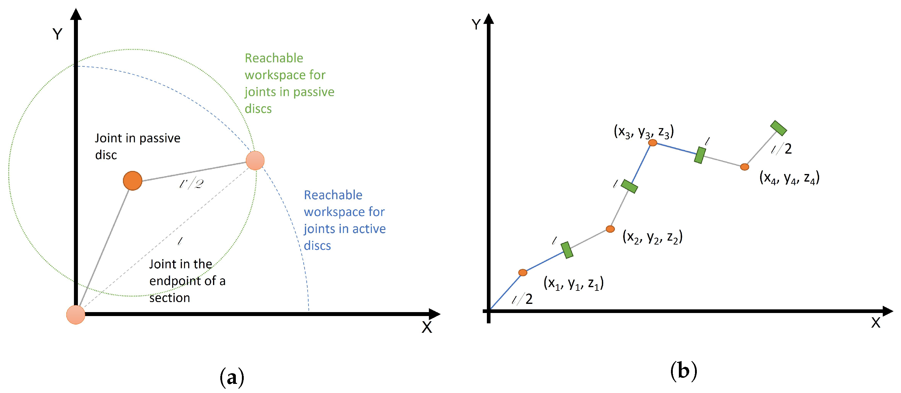
Modelling the robot as a kinematic chain of spherical joints, in [26], it is expressed how to directly apply this CCD algorithm to the inverse kinematics of hyper-redundant robots. In order to simplify the other steps of the modelling process, it is important to note that how these spherical joints are positioned in the robot affects the shape of the reachable space. To understand this, an example with discrete robots is provided. Since most algorithms return the pose of the spherical joints, it can be intuitively proposed to fix them to each section’s endpoint (their pose would then already be determined).

Two possible reachable spaces are defined, depending on the position of the joints relative to the studied section. If the physical joint in a discrete robot is placed in the endpoint of a section (in the centre of an active disc), a certain workspace is defined. However, if the robot has a rigid union between joints, which are placed inside a passive disc, the possible endpoint positions are conditioned by the orientation of the previous straight segment. (See Figure 19a).

In discreet robots, it is clear that virtual joints should be modelled to represent the physical reality of the robot. Most hyper-redundant robots have joints placed in the middle of the section, inside passive discs, and as such, that model is more accurate. In fact, in Figure 19b, the possible model for a discreet robot can be found. Green rectangles represent the endpoint of a certain section, and orange circles are the symbols for joints. As it can be seen, the transition between sections is performed by straight segments and, as such, the orientation of its endpoint depends directly on the previous joint. Calling the joints’ positions ${\left[\begin{array}{ccc}{x}_k& y_k& z_k\end{array}\right]}^t$ and ${\left[\begin{array}{ccc}{x}_{ek}& y_{ek}& z_{ek}\end{array}\right]}^t$ the endpoints, Equation (77) represents this transformation.

$$\left[\begin{array}{c}{x}_{ek}\\ y_{ek}\\ z_{ek}\end{array}\right]=\left[\begin{array}{c}\frac{x_{k+1}-x_k}{2}\\ \frac{y_{k+1}-y_k}{2}\\ \frac{z_{k+1}-z_k}{2}\end{array}\right]$$

(77)

On the other hand, continuous robots are modelled equivalently, with joints and straight lines, but the definition of these virtual elements is not straightforward. In fact, any of the two models seen in Figure 19a may be applied, as they are exchangeable through an additional degree of freedom (sections’ length) and the definition of another constraint. A common approach used in continuous robots is extending the concepts from discreet robots to continuous configurations, thus using the same definitions (virtual joints in the middle of the section in order to position the endpoint). However, this could be particular for each case, depending on the physical robot’s characteristics.

It must be reminded, however, that the simplifying hypothesis might introduce new equations that reduce the degrees of freedom. For example, the PCC hypothesis requires the length of the backbone to be constant, thus reducing the reachable space. These restrictions must be programmed into the optimisation algorithm.

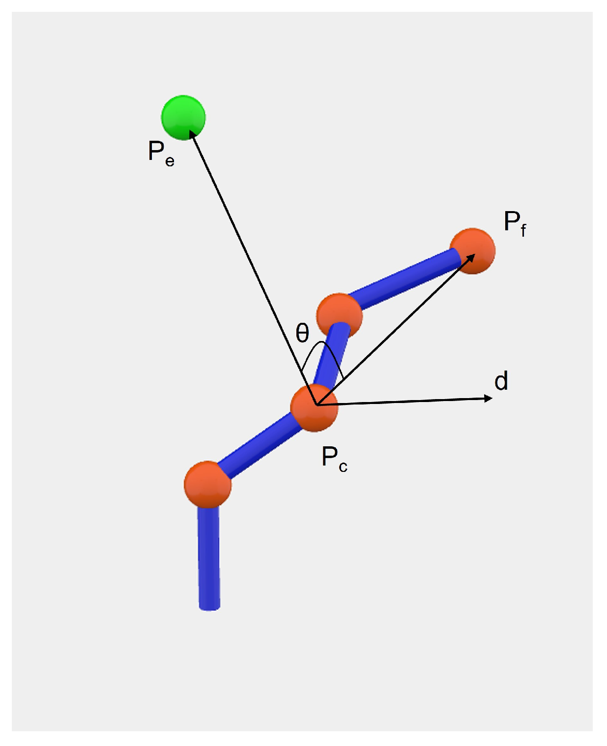
After having decided how to define the kinematic chain for the robot, the actual CCD algorithm is now tackled. To do so, three points are defined (see Figure 20): $p_c$ as the joint that is moved in a certain moment, or Current Joint; $p_e$ as the endpoint of the robot, or End-Effector; and finally $p_f$ as the final position that represents the objective for our inverse kinematic problem.

Using these three vectors, it can easily be deduced that in order to minimise the distance $\left|\right|\overrightarrow{p_e{p}_f}\left|\right|$, the vectors $\overrightarrow{p_c{p}_e}$ and $\overrightarrow{p_c{p}_f}$ should become aligned. This rotation could be represented by an angle $\theta$ and a direction $\overrightarrow{d}$ to indicate the rotation axis. The expressions for each of these values are:

$$\theta ={cos}^{-1}\left(\frac{p_e-p_c}{\left|\right|\overrightarrow{p_c{p}_e}\left|\right|}·\frac{p_f-p_c}{\left|\right|\overrightarrow{p_c{p}_f}\left|\right|}\right)$$

(78)

$$\overrightarrow{d}=\frac{p_e-p_c}{\left|\right|\overrightarrow{p_c{p}_e}\left|\right|}·\frac{p_f-p_c}{\left|\right|\overrightarrow{p_c{p}_f}\left|\right|}$$

(79)

Successively applying these equations to joints $i=1,2,\cdots ,n$, several angles ${\theta }_i$ and the directions around which they must turn in order to achieve the endpoint’s final position are found. Afterwards, it is necessary to use the geometric relationships, given the hypothesis that joints are virtually linked together by a straight segment, so as to find the final position vector for each of the sections. Once these points are defined, the second step for the inverse kinematic can be applied.

As it was already stated in Section 2.3, one of the main advantages of this method, apart from its computational efficiency and its precision, is that it is a method that can be applied independently of the robot’s morphology, due to the fact that the particularisation for each type of robot is easily achieved, having already stated common models for the robots.

However, this method also presents several disadvantages which must be taken into account [26]. Kinematic singularities that might appear due to the design of the robot are not even considered in the CCD algorithm. Moreover, it does not include any collision manager, not even with itself. This might result in a planned movement that is impossible to carry out. Finally, operating with high values of $\theta$ can be quite demanding for the robot’s joints.

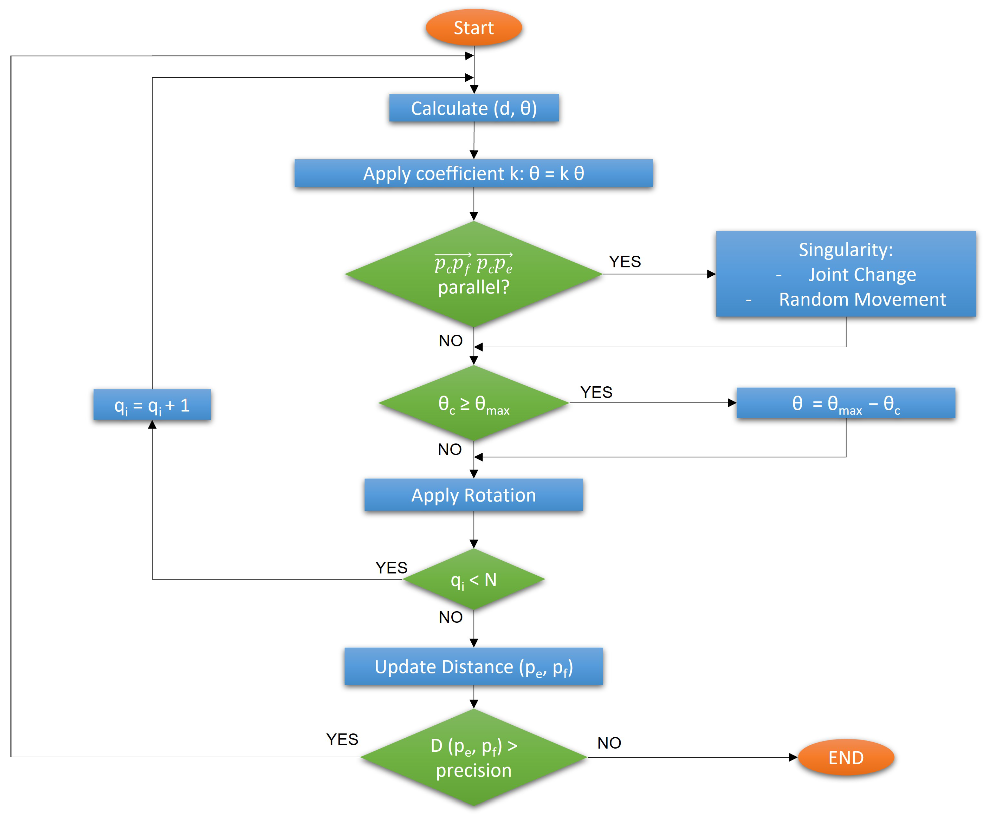
In order to solve, or at least mitigate these inconveniences (which might negatively affect the CCD algorithm usage), the Natural-CCD was developed [26]. Natural-CCD is an algorithm derived directly from CCD which obtains better results and more natural movements for the robot. This modification solves the CCD problems one by one:

• To tackle the possibility of a singularity, two viable alternatives can be used. In some cases, it would be enough to change to another joint (the movement of one of the joints might exit by itself the singularity that the first joint caused). However, in some cases where the singularity affects the whole robot (as when the robot is perfectly colinear and pointing to the goal), the Natural-CCD algorithm assigns a random d and $\theta$ that exit the position and allow it to continue.
• Collision management with itself is solved by designing an angle ${\theta }_{max}$ that represents a maximum bound for the possible range of the joint. This way, the angle can be defined so the segment can never collide with its predecessor. To do so, Martín et al. in [26] define ${\theta }_{max}$ as the supplementary angle to the interior angle of an N-sided polygon, N being the number of the robot’s joints.
• Finally, to minimise the effect of abrupt movements to the joints, Natural-CCD limits by a coefficient k the value of ${\theta }_i$ for the rotation. Particularly, the inverse of the distance between the robot’s endpoint and the desired position is suggested as a possible coefficient. However, k must be superiorly bounded by 1 in order for the algorithm to converge.

  $$k=\frac{1}{|\overrightarrow{p_e{p}_f}|}0>k\ge 1{\theta }^{*}=k\theta$$

Another possible definition for the coefficient k is based on trying to obtain a specific number of cycles for a certain movement. To do so with N being the number of joints and C a positive constant:

$$k=\frac{C}{N|\overrightarrow{p_e{p}_f}|}0>k\ge 1{\theta }^{*}=k\theta$$

These modifications are the basis of the final Natural-CCD algorithm. In Figure 21 a graphical summary can be found with said procedure.

Using this algorithm implies some interesting consequences. Firstly, from Natural-CCD more natural movements are obtained, with fewer sudden movements. In fact, Natural-CCD can be considered to produce a certain biomimetic action [26]. Moreover, modifying the algorithm by changing the chosen points for its development ($p_e,p_c,$ and $p_f$) surprisingly develops certain behaviours that, autonomously, might represent a functionality such as folding around itself, straightening, moving away from a point, etc. [45].

In this work, the Natural-CCD algorithm is suggested as a possible algorithm for section positioning due to its simplicity and the advantages it presents regarding computational efficiency and its real-time behaviour. However, many alternatives exist that are being used for hyper-redundant kinematics.

To show this, the inverse kinematic problem could be presented as trying to minimise the distance of the robot’s endpoint to the objective, while verifying certain restrictions. This, at its core, is an optimisation problem. Therefore, to solve the section positioning problem, any optimisation algorithm could be used, including Neural Networks or Deep Learning techniques. The choice between these alternatives might depend on the computational power available, the response-time requirements or even the designer’s personal preferences ([23,24,25]).

8. Tutorial for Hyper-Redundant Robot Modelling

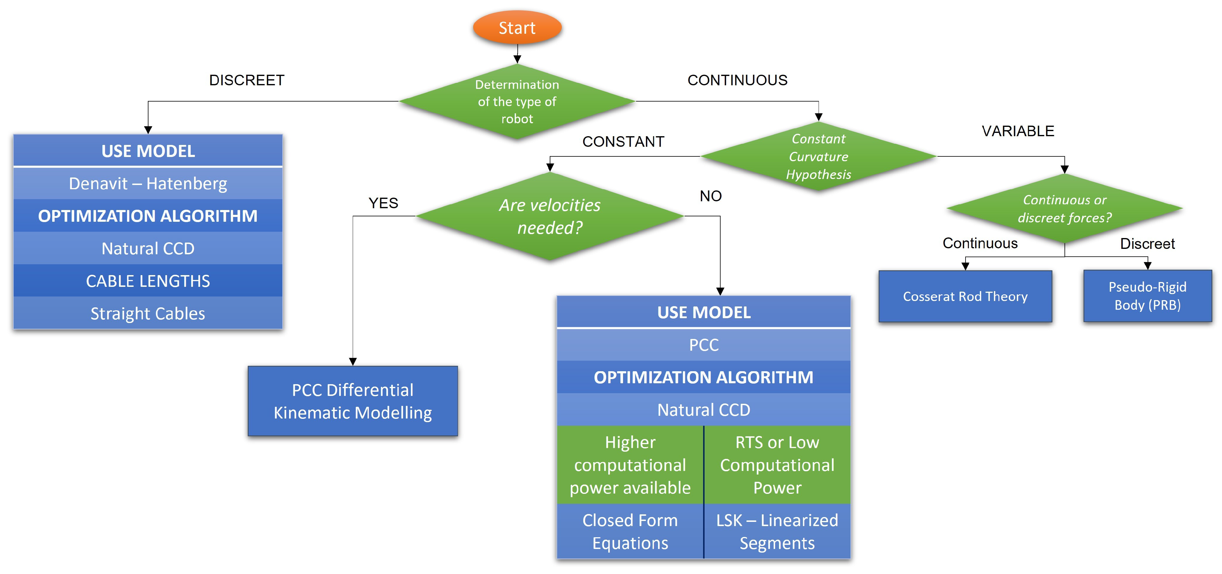
Once some of the most important techniques for hyper-redundant kinematic modelling have been revised, this paper aims to offer some guidelines for the engineer that first approaches this topic. The proposal uses the classification given in Section 1.2 to make decisions between the existing alternatives.

A graphical summary is presented in Figure 22 as it is the basis for the explanations given in this section. In the following subsections, the different steps that are proposed in the procedure are explained in further detail. For example, it is reviewed how to decide whether or not a robot is discreet or continuous and how to determine if the backbone is constant or variable.

8.1. Determination of the Type of Robot

The first step in order to conceive the kinematic model of a hyper-redundant robot is to determine the type of robot that will be modelled. As it has been stated throughout the revision of the different methods, it is an essential factor when deciding which approach is best for a certain robot.

The main difference in the model selection is the discreetness or continuousness of the robot’s joints. If the robot is a kinematic chain of several joints with one or two DOF, then the Denavit–Hartenberg method would be perfect for obtaining the kinematic equations. However, if the backbone is purely continuous, then other factors must be considered when modelling.

Cable lengths also depend on this decision. In fact, it is a very determining factor. When the robot is continuous (or can be approximated as such) cable lengths are far more difficult to model, and usually PCC and Closed Forms equations are needed so as to include the intermediate passive discs in the mathematical expressions.

Moreover, if there are no passive discs, cables would form a straight line between sections, and the Denavit–Hartenberg method could be directly applied (it has already been stated that this method could be used to obtain curvature parameters).

8.2. Example of Discreet Robot: MACH-I

An example of a discreet robot is MACH-I. It can clearly be seen that it consists of several discreet joints between sections (see Figure 23a,b). In fact, cables do follow a straight line between sections. The only thing that must be taken into account is that sections do have a certain width that must also be added to the cable length.

Having classified MACH-I as a discreet CDHR, the kinematic modelling technique that is proposed is the Denavit–Hartenberg method. It is fairly simple and can be used with the Natural-CCD algorithm to enable inverse kinematics. Some particularities of the robot should be taken into account, such as the straight segment of cable there is between sections.

In fact, the choice of the Denavit–Hartenberg parameters is quite similar to that made in Section 3. The defined reference frames can be seen in Figure 24a, while the parameters are in Figure 24b. In addition to these transformations, the base and endpoint reference frames must also be added through two rotations (Equations (80) and (81)):

$${}^B{\mathit{A}}_0=\mathit{T}(0,0,L+H/2){\mathit{Rot}}_y(-\pi /2)$$

(80)

$${}^2{\mathit{A}}_F={\mathit{Rot}}_y(\pi /2){\mathit{Rot}}_z(\pi /2)$$

(81)

Therefore, the simple section transformation is found in Equation (82) by multiplying all the correspondent matrices obtained by the Denavit–Hartenberg method.

$$S_i=\mathit{T}(0,0,L+H/2){\mathit{Rot}}_y{(-\pi /2)}^1{\mathit{A}}_2^2{\mathit{A}}_3{\mathit{Rot}}_y(\pi /2){\mathit{Rot}}_z(\pi /2)$$

(82)

Each section endpoint can be found by multiplying all the preceding sections’ matrices.

$$S_n=S_1·S_2·\cdots ·S_{n-1}·S_n$$

(83)

Having achieved this, inverse kinematics demonstrate themselves to be quite easy. The first step would involve using the Natural-CCD algorithm to locate the endpoint reference frame for each section. Defining the two degrees of freedom of each joint as said parameters $q_1$ and $q_2$ would directly return these values for each section. Then, transforming this information into cable lengths is easy, since the transformation matrices would already be available. However, further geometric reasoning is needed (see Figure 25).

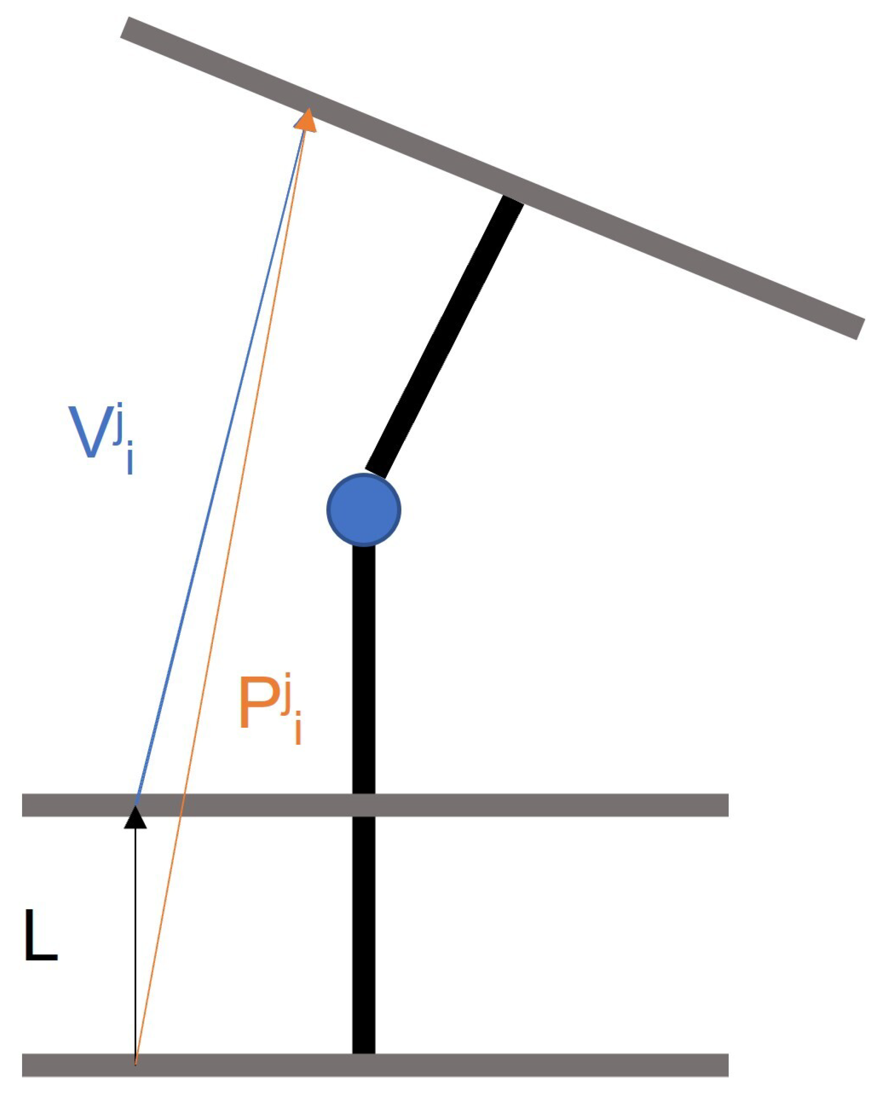
For each section, the endpoint position of each of the cables can be easily calculated by applying the transformation matrix of said section to the origin of the cable. For example, for section j, knowing cable i is located in point $(0,d,0)$, its end ($P_i^j$) would be located at:

$$P_i^j=S_1·\left[\begin{array}{c}0\\ d\\ 0\end{array}\right]$$

(84)

It must be taken into account that this vector includes both the fixed length of the cable (L) and the variable length ($V_i^j$) due to the current position. Therefore, the fixed part is subtracted knowing the current vector is obtained in section coordinates, and the section always starts oriented towards the z axis:

$$V_i^j=P_i^j-\left[\begin{array}{c}0\\ 0\\ L\end{array}\right]$$

(85)

The final length is then obtained using the sum of the fixed and the variable part:

$$l_i^j=L+\parallel V_i^j\parallel$$

(86)

Recursively calculating each section’s cable lengths allows to add up the total length of each cable. Another alternative is to use increments of cable, for which fewer operations are needed. A complete inverse kinematic model is available for the MACH-I with these equations.

In case a direct kinematic model is needed, the relationships between the lengths of the cables and the degrees of freedom used in Denavit–Hartenberg’s equations (the angles around x and y axis) would be required. As a parallel robot PPP-3S, the calculations are not direct, and would require either numerical algorithms or artificial intelligence to obtain them [46].

8.3. Constant Curvature Hypothesis

When considering continuous robots, the determining step (which might not be as easy as it seems) is deciding whether the constant curvature hypothesis applies to the robot to be modelled. The consequences of this dilemma directly affect the difficulty of the modelling process.

No robot actually complies perfectly with the constant curvature hypothesis. Therefore, the definitive criteria for rejecting the constant curvature hypothesis would be the empiric trials to determine whether the error is excessive, and thus the model must be rejected if the error is negligible or if it can be corrected by the controller.

As stated in Section 6, some of the reasons for the hypothesis not being applicable include an excessive weight of the robotic structure or not enough stiffness in the material. In these cases, a dynamic model is necessary. Whenever this is the case, a further question could be asked: whether or not the forces applied to the robot can be considered continuous (therefore using the CRT method) or discreet (where the PRB model is useful).

8.4. Example of Non-PCC Robot: Ruan

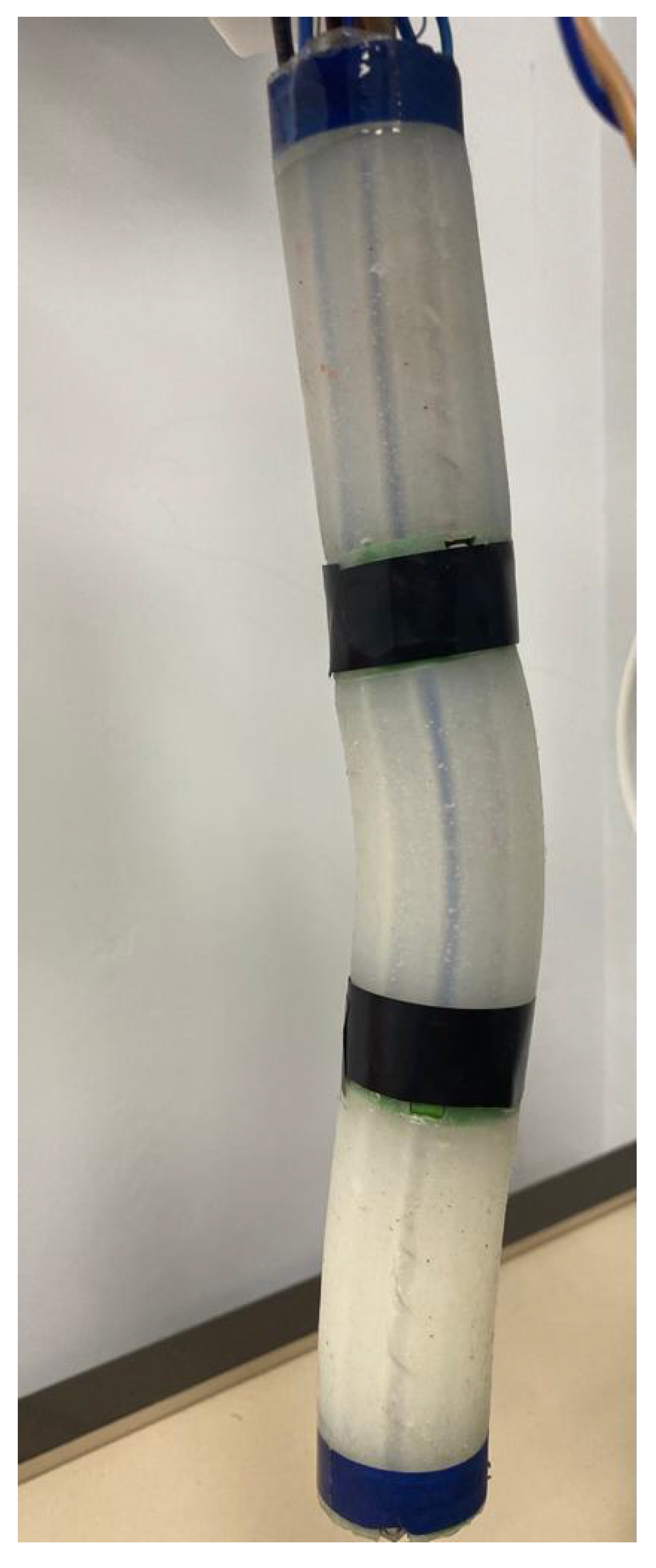
A good example of a robot which could be excluded from the constant curvature hypothesis is the previously introduced Ruan Robot. Ruan is a soft robot (see Figure 26). It can easily be stated that it does not belong to the discreet category, which directly excludes Denavit–Hartenberg method as applied to MACH-I.

Ruan being a soft robot implies that the constant curvature hypothesis may not be accurate enough when establishing its mathematical equations. Therefore, other alternatives such as the PRB or the Crosserat Rod Theory could be tried, depending on the knowledge of internal and external strains and forces. In the case of this soft robot, due to the fact that SMA threads act upon the discreet discs, the PRB method is proposed. Numerical methods, such as Finite Element Methods are also very common for soft robotics.

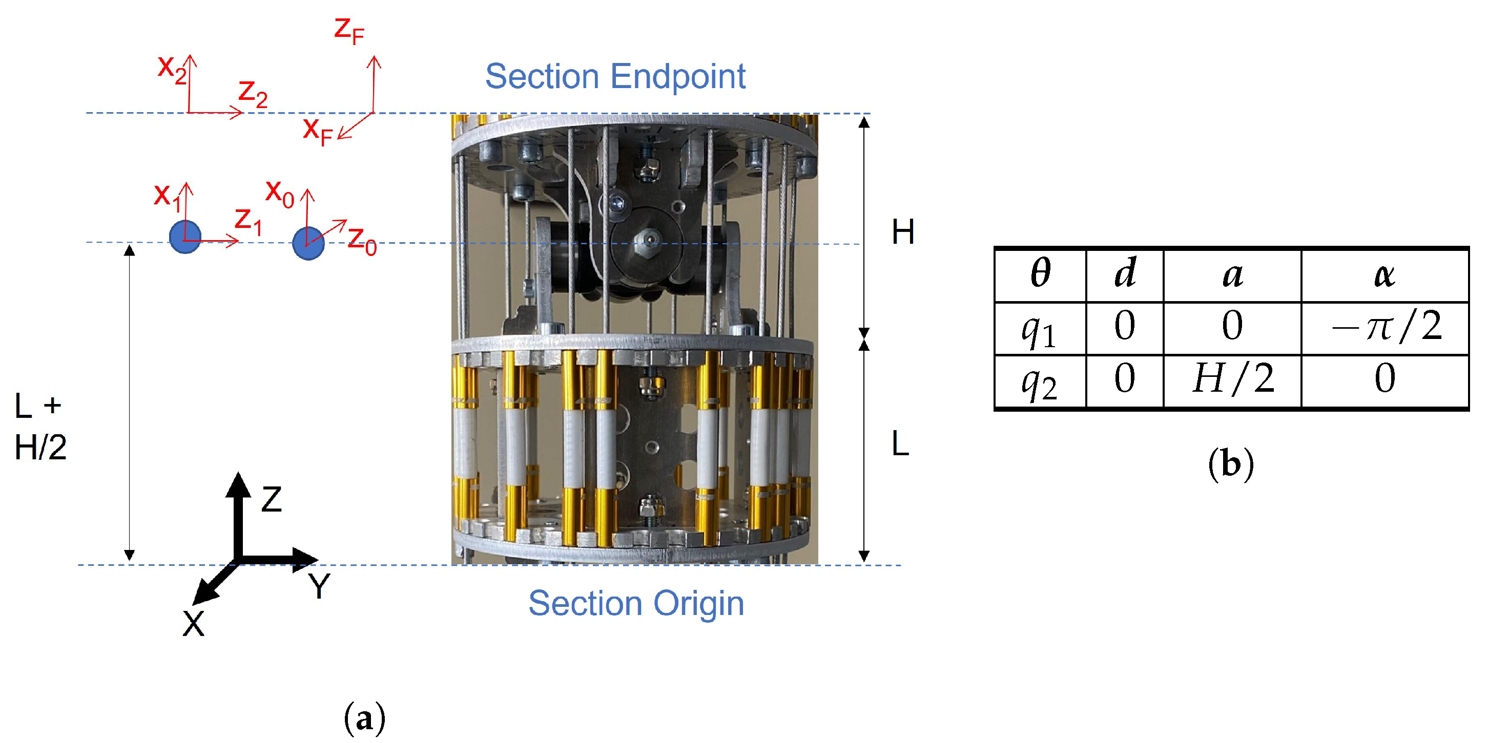
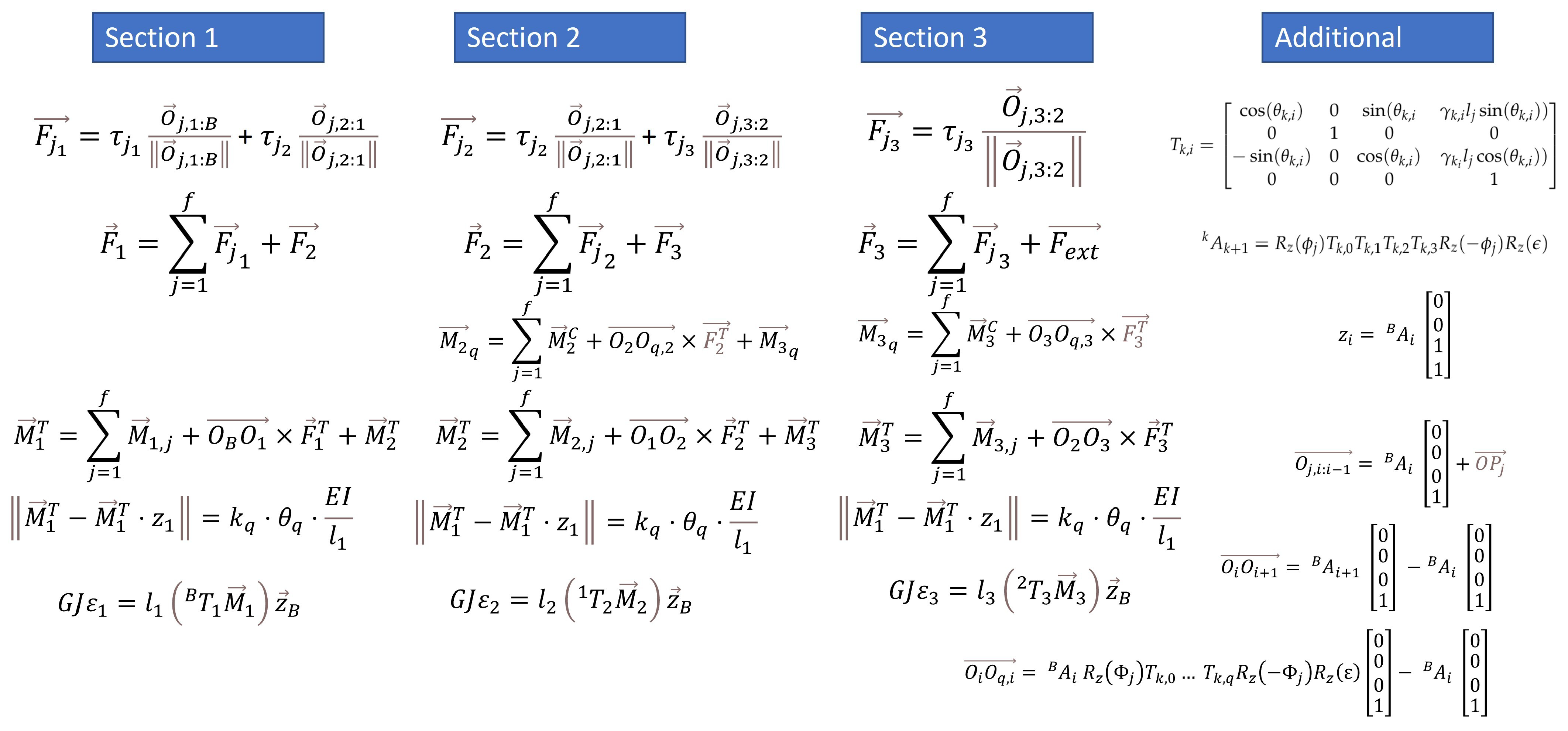
As said, the PRB method can be applied to this case. It is a three-disc robot, so three sections for the PRB need to be considered. Equations can be found in Figure 27. In addition to these equations, some general expressions must be added in order to transform some variables into known information (external forces and the tension of the cables).

This lot of equations would then have to be inserted into a nonlinear solver in order to update the position of the robot at each time, according to the PRB robot.

8.5. Inside the PCC Model

Apart from the aforementioned factors, there are some considerations that might help to choose a particular set of equations for a hyper-redundant robot that complies with the PCC hypothesis. For example, whenever the velocities are relevant information for the model (either because the sensors capture them or because the researcher is interested in developing a speed control system), the right choice would be to develop a differential model.

Computational power should also be taken into account. Hyper-redundant robots with many sections greatly increase the number of operations that are needed to solve the kinematic equations. Therefore, a less costly technique is more advisable than Closed-Form Equations. When a Real-Time System is also desirable, it also helps to reduce the number of operations. Linearisation allows faster computation and substantially less memory required for each DOF, thus being the best option when resources are scarce.

For example, MACH-I is designed to work with a computer next to it, which sends the instructions and can calculate simultaneously. Since a standard PC has enough computational power, even having several cores for parallel computing, it could implement the classical equations without worrying much about the scarcity of resources.

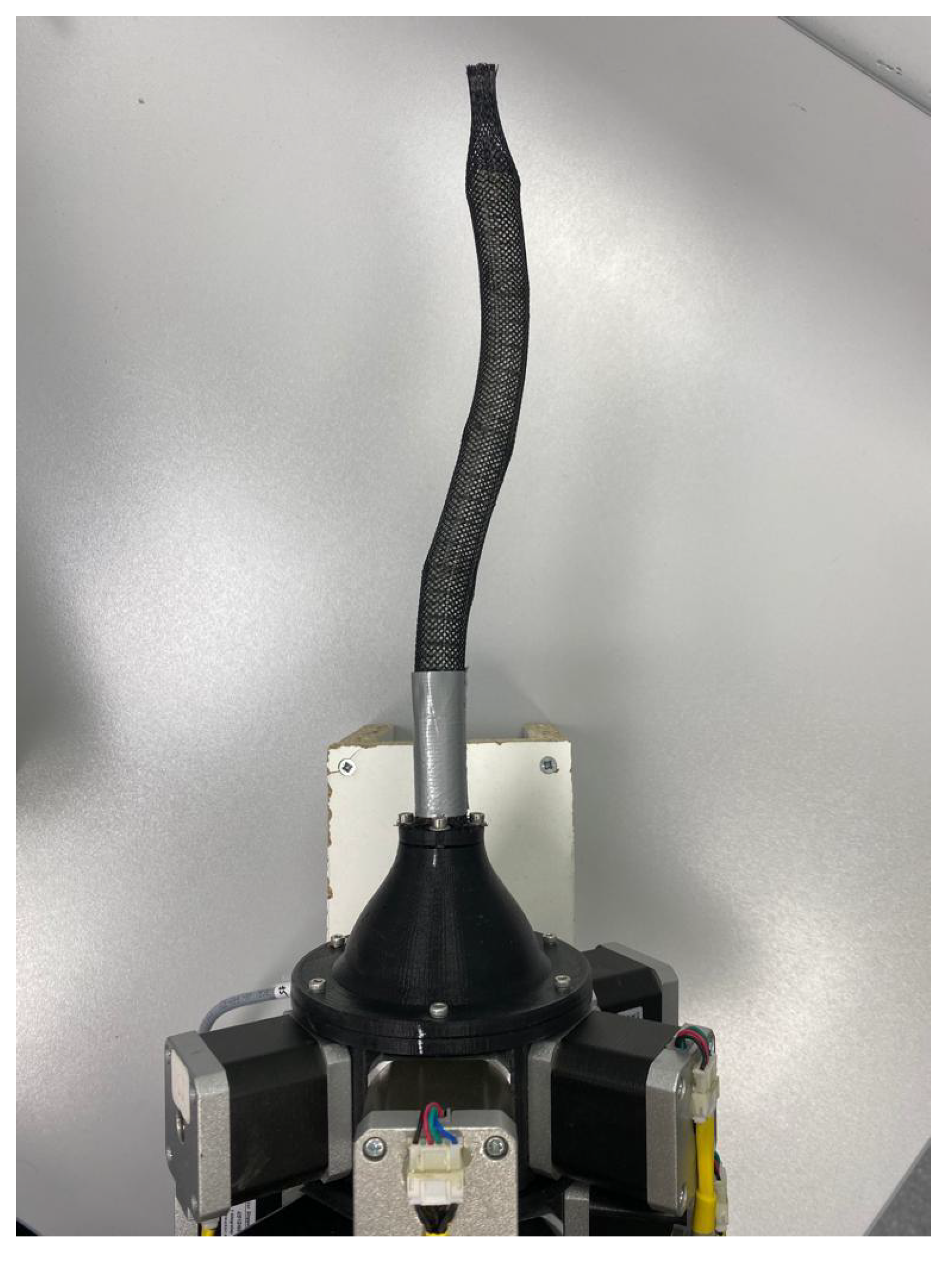
8.6. Example of PCC Robot: Pilory

As an application example for this decision, the Pilory robot can be used (see Figure 28). Beginning again with the classification process, the Pilory robot has a disc structure where one disc pivots over the following. It has four sections, with 20, 12, 12 and 8 discs each [20]. Every section is then actuated by four cables. There are no distinguishable discreet joints, and between sections, there are many intermediate passive discs. Therefore, the Denavit–Hartenberg method for discreet robots is immediately discarded.

Pilory has no backbone, therefore it has no problems with elasticity. It is quite lightweight since it has been built with 3-D-printed discs. These features account for trying to apply the constant curvature hypothesis before proceeding to more complex models, since it is not a soft robot, and the mathematical model might be good enough.

Inside the PCC model, the decisions can be considered more arbitrary. In this case, the simplest model is sought after, and velocities are not considered a must. This is why a differential model is not a requirement, and a simpler and more intuitive model is chosen.

The final decision in the proposed tutorial is whether or not the robot has low computational power, or if it is designed for real-time operation. The robot is managed through some hardware drivers that translate the instructions to the necessary electrical impulses, but the control is completely calculated by an external computer, which is connected to the hardware by a USB serial. The external computer has enough calculation power to use the complete model. Moreover, the robot is academically used and has no need for RTS features. Therefore, it is decided not to use the LSK method.

Therefore, the proposed model for Pilory (see Figure 29) is using PCC equations (as obtained in Section 4) for direct kinematics. Additionally, closed-form equations combined with the Natural CCD algorithm would be used for inverse kinematics.

9. Conclusions

As it has been revised in this work, hyper-redundant robotics is a growing sector that can be approached from different perspectives. Some mathematical alternatives are offered to the novel researcher, although it might be confusing to further reflect on some of them due to the large amount of work being published.

This article offers some guidelines to understand the current bibliography: It develops a simple scheme to conceptually fit all the models that are presented here, using several transformations to obtain both the direct and inverse kinematics for hyper-redundant robots. It also suggests a possible route in order to decide which mathematical expressions can be more useful depending on some of the robot’s characteristics. This would simplify the approximation to the topic for newcomers while showing some of the most important differences between the methods available.

The proposal of a method of decision when tackling hyper-redundant robot modelling was applied to some examples of real robots, which also helps to clarify the concepts, and it provides a practical case for the novel researcher that approaches this topic.