Using Probabilistic Models for Data Compression

Abstract

Our research objective is to improve the Huffman coding efficiency by adjusting the data using a Poisson distribution, which avoids the undefined entropies too. The scientific value added by our paper consists in the fact of minimizing the average length of the code words, which is greater in the absence of applying the Poisson distribution. Huffman Coding is an error-free compression method, designed to remove the coding redundancy, by yielding the smallest number of code symbols per source symbol, which in practice can be represented by the intensity of an image or the output of a mapping operation. We shall use the images from the PASCAL Visual Object Classes (VOC) to evaluate our methods. In our work we use 10,102 randomly chosen images, such that half of them are for training, while the other half is for testing. The VOC data sets display significant variability regarding object size, orientation, pose, illumination, position and occlusion. The data sets are composed by 20 object classes, respectively: aeroplane, bicycle, bird, boat, bottle, bus, car, motorbike, train, sofa, table, chair, tv/monitor, potted plant, person, cat, cow, dog, horse and sheep. The descriptors of different objects can be compared to give a measurement of their similarity. Image similarity is an important concept in many applications. This paper is focused on the measure of similarity in the computer science domain, more specifically information retrieval and data mining. Our approach uses 64 descriptors for each image belonging to the training and test set, therefore the number of symbols is 64. The data of our information source are different from a finite memory source (Markov), where its output depends on a finite number of previous outputs. When dealing with large volumes of data, an effective approach to increase the Information Retrieval speed is based on using Neural Networks as an artificial intelligent technique.

1. Introduction

The assessment of similarity or distance between two information entities is crucial for all information discovery tasks (whether Information Retrieval or Data mining). Appropriate measures are required for improving the quality of information selection and also for reducing the time and processing costs [1].

Even if the concept of similarity originates from philosophy and psychology, its relevance arises in almost every scientific [2]. This paper is focused on measuring similarity in the computer science domain, i.e., Information Retrieval, in images, video, and to some extent audio, respectively. In the paper domain, the similarity measure “is an algorithm that determines the degree of agreement between entities.” [1].

The approaches for computing similarity or dissimilarity between various object representations can be classified [2] in:

(1)

distance-based similarity measures

This class includes the following models: Euclidean distance, Minkowski distance, Mahalanobis distance, Hamming distance, Manhattan/City block distance, Chebyshev distance, Jaccard distance, Levenshtein distance, Dice’s coefficient, cosine similarity, soundex distance.

(2)

feature-based similarity measures (contrast model)

This method, proposed by Tversky in 1977, represents an alternate to distance-based similarity measures, based on computing similarity by common features of compared entities. Entities are more similar if they share more common features, while they are dissimilar in the case of more distinctive features. The similarity between entities A and B can be determined using the formula:

$$s(A,B)=\alpha g(A\cap B)-\beta g(A-B)-\gamma g(B-A),$$

(1)

where:

–

$\alpha ,\beta ,\gamma$ are used to define the respective weights of associated values,

–

$g(A\cap B)$ describes the common features in A and B,

–

$g(A-B)$ stands for the distinctive features of A

–

$g(B-A)$ means the distinctive features of the entity B.

(3)

probabilistic similarity measures

For assessing the relevance among some complex data types, the following probabilistic similarity measures are necessary: maximum likelihood estimation, maximum a posteriori estimation.

(4)

extended/ additional measures

Includes similarity measures based on fuzzy set theory [3], similarity measures based on graph theory, similarity-based weighted nearest-neighbors [4], similarity-based neural networks [5].

A lot of algorithms and techniques like Classification [6], Clustering, Regression [7], Artificial Intelligence(AI), Neural Networks (NNs), Association Rules, Decision Trees, Genetic Algorithm, Nearest Neighbor method etc., are attempted [2] for knowledge discovery from databases.

The Artificial Neural Networks (ANNs) are widely used in various fields of engineering and science. They generate useful tools in quantitative analysis, due to their unique feature of approximating complex and non-linear equations. Their performance and advantage consists in their ability to model both linear and non-linear relationships.

The Artificial Neural Networks are well-suited for a very broad class of nonlinear approximations and mappings. An Artificial Neural Network (ANN) with nonlinear activation functions is more effective than linear regression models in dealing with nonlinear relationships.

ANNs are regarded as one of the important components in AI. They have been studied [8] for many years with the goal of achieving human-like performance in many branches, such as classification, clustering, and pattern recognition, speech and image recognition and Information Retrieval [9] by modelling the human neural system.

IR “is different from data retrieval in databases using SQL queries because the data in databases are highly structured and stored in relational tables, while information in text is unstructured. There is no structured query language like SQL for text retrieval.” [10].

Gonzales and Woods [11] have developed Huffman Coding to remove coding redundancy, by yielding the smallest number of code symbols per source symbol.

Burgerr and Burge [12] as well as Webb [13] have developed several algorithms for Image Compression using Discrete Cosine Transformation.

The main objective of this paper consists in improving the performance of the Huffman Coding algorithm by achieving a minimum average length of the code word. Our new approach is important for removing more effectively the Coding Redundancy in Digital Image Processing.

The remainder of the paper is organized as follows. In Section 2 we discuss some general aspects about the Poisson distribution and the data compression.

Then, in Section 3 we introduce and analyze an approach to reduce the documents, entitled Discrete Cosine Transformation, in order to achieve the Latent Semantic Model.

We follow with the Fourier descriptor method in Section 4 to describe the shape of an object by considering its boundaries.

We define some notions from the Information Theory in Section 5 as they are useful to model the information generation like a probabilistic process.

The Section 6 presents the Huffman Coding, which is built to remove the coding redundancy and to find the optimal code for an alphabet of symbols.

We introduce an experimental evaluation of the new model on the task of computing image entropy, the average length of the code words and the Huffman coding efficiency too in Section 7.

We conclude in Section 8 by highlighting that the scientific value added by our paper consists in the fact of computing the average length of the code words in the case of applying of the Poisson distribution.

2. Preliminaries

2.1. Discrete Random Variables and Distributions

By definition [14], a random variable X and its distribution are discrete if the possible values of X denoted $x_1,x_2,x_3,\cdots$ are finitely many or, at most, countably many values, with the probabilities $p_1=P(X=x_1),p_2=P(X=x_2),p_3=P(X=x_3),\dots$.

The Poisson Distribution

The Poisson distribution (named after S.D. Poisson) is the discrete distribution which has infinite possible values and the probability function

$$P\left(k\right)=\frac{{\lambda }^k}{k!}{\mathrm{e}}^{-\lambda },\lambda >0.$$

(2)

The Poisson distribution is similar with the binomial distribution in the mean in that it is achieved as a limiting case of this distribution, for $n\to \infty$ and $p\to 0$, where the product $np=\lambda >0$ is kept constant. As it is used for a rare occurrence of an event, the Poisson distribution is also called the distribution of the rare events that occur in order to achieve success in a sequence of some independent Bernoulli samples.

This distribution is frequently encountered in the study of some phenomena in biology, telecommunications, statistical quality control (when the probability of obtaining a defect is very small), in the study of phenomena that present some agglomerations (in the theory of threads of waiting).

The probability that of the n drawn balls, k are white is: [15]

$$\begin{array}{c}P\left(k\right)={\displaystyle \underset{n\to \infty }{lim}}{P}_n\left(k\right)={\displaystyle \underset{n\to \infty }{lim}}{C}_n^k{p}^k{q}^{n-k}={\displaystyle \underset{n\to \infty }{lim}}{C}_n^k{\left(\frac{\lambda }{n}\right)}^k{\left(1-\frac{\lambda }{n}\right)}^{n-k}=\\ =\frac{{\lambda }^k}{k!}·\underset{=1}{\underbrace{{\displaystyle \underset{n\to \infty }{lim}}\frac{n!}{n^k(n-k)!}}}·\underset{{\mathrm{e}}^{-\lambda }}{\underbrace{{\displaystyle \underset{n\to \infty }{lim}}{\left(1-\frac{\lambda }{n}\right)}^{n-k}}},\end{array}$$

namely it results in the Equation (2).

The simulation of $X\sim Po\left(\lambda \right)$ can be achieved [16,17]: using the Matlab generator, using the inverse transform method, using a binomial distribution.

In [17] we generated a selection of volume 1000 on the random variable X, having some continuous distributions (such as normal or exponential distribution) or discrete distributions (as the geometric or Poisson distribution). The methods used in the generation of the random variables X are illustrated in the

Table 1. The methods used to generate a selection of volume 1000 on the random variable X, having some continuous and discrete distribution.

Random Variable	Simulation Method	Mean		Variance		Statistics
						${\mathbf{\chi }}^{\mathbf{2}}$	Kolmogorov
Normal	Matlab	2	1.9392	4	3.9472	54.3986	0.0143
	Box-Muller	2	2.0216	4	4.1625	42.7415	0.0101
	Rejection polar	2	2.0706	4	4.0830	28.4396	0.0176
Exponential	Matlab	1	1.036	1	1.03	136.3055	0.0249
	Inverse method	1	0.9657	1	0.9786	102.8223	0.0193
	Gamma distribution	1	1.01	1	1.01	108.6551	0.0253
Geometric	Matlab	2.3333	2.327	7.7778	7.4535	56.9155	0.05
	Inverse method	2.3333	2.763	7.7778	7.6825	34.6667	0.0408
	Counting the failures	2.3333	2.361	7.7778	7.7664	39.6033	0.0454
Poisson	Matlab	1	0.999	1	0.964	21.1409	0.049
	Binomial distribution	1	1.038	1	0.0977	39.0964	0.039

.

The means and the variances corresponding to the resulting selections will be compared with the theoretical ones. In each case we build both the graphical histogram and the probability density of X too. For example, the Figure 1 shows the histograms built for $X\sim Geom\left(p\right)$, using three methods (Matlab generator, inverse transform method, by counting the failures) and the probability density of X.

The statistics associated to the concordance tests are also computed in the Table 1.

Example 1.

Adjust the following empirical distribution, which is a discrete one, using the Poisson distribution:

$x_i$	0	1	2	3	4	5	6	7	8	9
$P\left(x_i\right)$	0.16	0.217	0.27	0.18	0.11	0.03	0.1	0.002	0.001	0.002

The resulting Poisson distribution will be:

x	0	1	2	3	4	5	6	7	8	9
$P\left(x\right)$	0.0799	0.2019	0.2551	0.2149	0.1358	0.0686	0.0289	0.0104	0.0033	0.0009

2.2. Data Compression

The concept of data compression [11,18,19,20,21,22,23,24,25,26,27,28] means the reduction of that amount of data, which is used to represent a given quantity of information.

The data represent the way in which the information is transmitted, such that different amounts of data can be used to represent the same quantity of information.

For example, if $n_1$ and $n_2$ are the number of bits in two representations of the same information, then the relative data redundancy $R_D\in (-\infty ,1)$ of the representation with $n_1$ bits can be defined as:

$$R_D=1-\frac{1}{C_R},$$

(3)

where $C_R\in (0,\infty )$ signifies the compression ratio and has the expression:

$$C_R=\frac{n_1}{n_2}.$$

(4)

There are the following three types of redundancies [11] in the Digital Image Processing:

(A)

Coding Redundancy- it is necessary to evaluate the optimal information coding by the average length of the code words ($L_{avg}$) to remove this kind of redundancy:

$$L_{avg}=\sum _{k=0}^{L-1}l\left(r_k\right)p_r\left(r_k\right),$$

(5)

where:

✓

L being the number of the intensity values associated to a an $M\times N$ image;

✓

$MN{L}_{avg}$ bits are necessary to represent the respective $M\times N$ image;

✓

the discrete random variable $r_k\in [0,L-1]$ represents the intensities of that $M\times N$ image;

✓

$n_k$ is the absolute frequency of the k- th intensity $r_k$;

✓

$l\left(r_k\right),k\in \overline{0,L-1}$ means the number of bits that are used to represent each value of $r_k$;

✓

$p_r\left(r_k\right)=\frac{n_k}{MN}$ is the probability of the occurrence of the $r_k$ value;

(B)

Interpixel Redundancy one refers to a reduction of the redundancy associated with spatially and temporally correlated pixels through mapping such as the run-lengths, differences between adjacent pixels and so on; reversible mapping implies the reconstruction without error;

(C)

Psychovisual Redundancy is when certain information which has relatively less importance for the perception of the image quality; it is different from the Coding Redundancy and the Interpixel Redundancy by the fact that it is associated with the real information, which can be removed by a quantization method.

3. Discrete Cosine Transformation

The appearance based approach constitutes [2] one of the various approaches used to select the features from an image, by retaining the most important information of the image and rejecting the redundant information. This class includes Principal Component Analysis (PCA), Discrete Cosine Transformation (DCT) [29], Independent Component Analysis (ICA) and Linear Discriminant Analysis (LDA).

In case of large document collections, the high dimension of the vector space matrix F generates problems in the text document set representation and induces high computing complexity in Information Retrieval.

The most often used methods for reducing the text document space dimension which have been applied in Information Retrieval are: Singular Value Decomposition (SVD) and PCA.

Our approach is based on using the Discrete Cosine Transformation for reducing the text documents. Thus, the set of keywords is reduced to the much smaller feature set. The resulting model represents the Latent Semantic Model.

The DCT [30] represents an orthogonal transformation, similar with the PCA. The elements of the transformation matrix are obtained using the following formula:

$$t_{mi}=\sqrt{\frac{2-{\delta }_{m-1}}{n}}cos\left(\frac{\pi }{n}(i-\frac{1}{2}(m-1))\right),(\forall )i,m=\overline{1,n},$$

(6)

n being the size of the transformation and

$${\delta }_m=\left\{\begin{array}{c}1\mathrm{if}m=1,\hfill \\ 0\mathrm{otherwise}.\hfill \end{array}\right.$$

(7)

The DCT requires the transformation of the n dimensional vectors $X_p,p=\overline{1,N}$, where N denotes the number of vectors that must be transformed), to the vectors $Y_p,(\forall )p=\overline{1,N}$, using the formula:

$$Y_p=T·X_p,(\forall )p=\overline{1,N},$$

(8)

$T={\left\{t_{mi}\right\}}_{i,m=\overline{1,n}}$ meaning the transformation matrix.

We have to choose, between all the components of the vectors $Y_p,p=\overline{1,N}$, a number of m components, corresponding to the positions which conduct to a mean square belonging to the first m mean squares, in descending order, while the other $n-m$ components will be cancelled.

The vector $Y_p,p=\overline{1,N}$, is defined through the formula (8):

$$Y_p=\left(\begin{array}{c}{y}_{p1}\\ ⋮\\ y_{pn}\end{array}\right).$$

The mean square of the transformed vectors is given by:

$$E\left(Y_p^2\right)=\left(\begin{array}{c}E\left(y_{p1}^2\right)\\ ⋮\\ E\left(y_{pn}^2\right)\end{array}\right),$$

(9)

where

$$E\left(y_{pj}^2\right)=\overline{y_{pj}^2}=\frac{1}{N}\sum _{p=1}^N{y}_{pj}^2,(\forall )j=\overline{1,n}.$$

The DCT application consists in determining the vectors ${\widehat{Y}}_p,p=\overline{1,N}$ corresponding to the m components of the vectors $Y_p,p=\overline{1,N}$ that do not cancel.

Image Compression Algorithm Using Discrete Cosine Transformation

Digital image processing represents [11,12,13,31,32] a succession of hardware and software processing steps, as well as the implementation of several theoretical methods.

The first step of this process involves the image acquisition. It requires an image sensor for achieving a two-dimensional image, such as a video camera (for example, the Pinhole Camera Model, one of the simplest camera models).

The analog signal (which is continuous in time and values) [33] resulted at the output of the video camera, must be converted into a digital signal, for its processing using the computer. This transformation involves the following steps [12]:  

Step 1 

(Spatial sampling). This step aims to achieve the spatial sampling of the continuous light distribution. The spatial sampling of an image represents the conversion of the continuous signal to its discrete representation and it depends on the geometry of the sensor elements associated to the acquisition device.

Step 2 

(Temporal sampling). In this stage, the resulting discrete function is sampled in the time domain to create a single image. The temporal sampling is achieved by measuring at regular intervals the amount of light incident on each individual sensor element.

Step 3 

(Quantization of pixel values). This step aims to quantize the resulting values of the image to a finite set of numeric values for storing and processing the image values on the computer.

Definition 1

 ([12]). A digital image I represents a two-dimensional function of natural coordinates $(u,v)\in \mathrm{N}\times \mathrm{N}$, which maps to a range of possible image values P, with the property that $I(u,v)\in P$.

The pixel values are described by binary words of length k (which define the depth of the image); therefore, a pixel can represent any of $2^k$ different values.

As an illustration, the pixels of the grayscale images:

• are represented by using k = 8 bits (1 byte) per pixel;
• have the intensity values belonging to the set $\{0,1,\dots ,255\}$, where the value 0 corresponds to the minimum brightness (black) and 255 represents the maximum brightness (white).

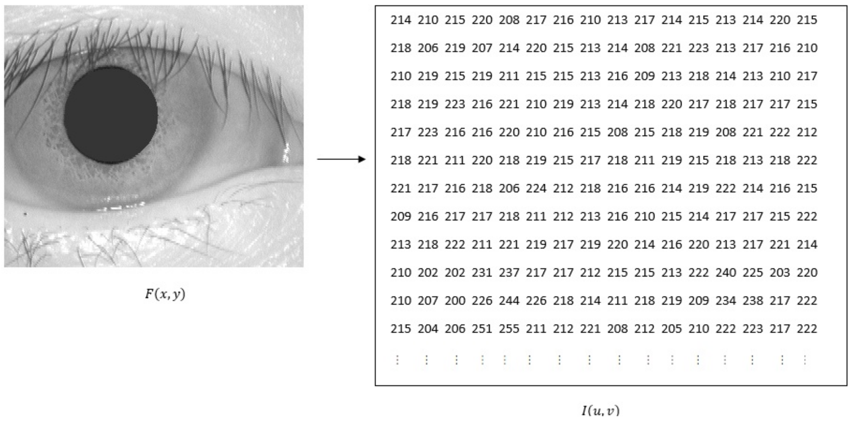
The result of performing the three steps Step 1–Step 3 is highlighted in a “description of the image in the form of a two-dimensional, ordered matrix of integers” [12], illustrated in the Figure 2.

CASIA Iris Image Database Ver 3.0 (or CASIA-IrisV3 for short) contains three subsets, totally 22,051 iris images of more than 700 subjects.

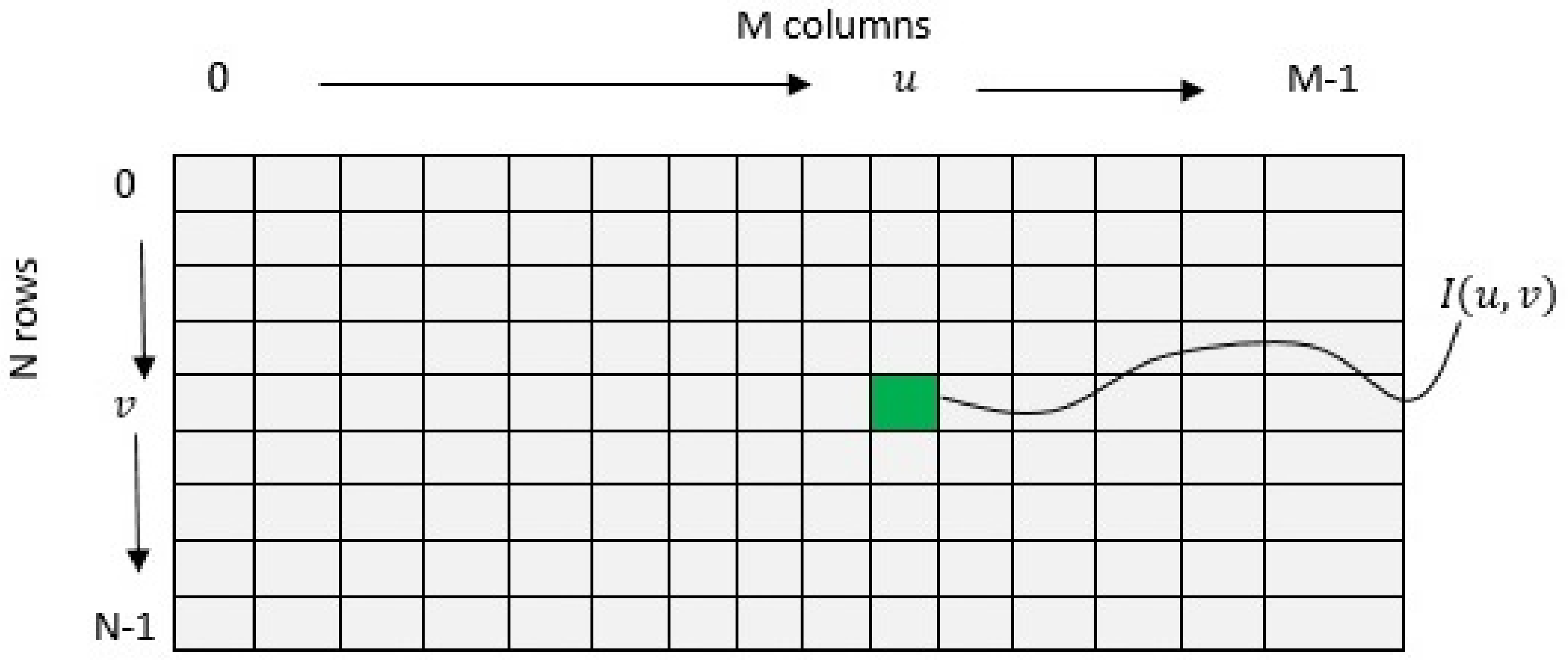
Figure 3 displays a coordinate system for image processing, which is flipped in the vertical direction, provided that the origin, defined by $u=0$ and $v=0$ lies in the upper left corner.

Another advantage of DCT in image compression consists in not depending on the input data.

The coordinates $u,v$ represent the columns and rows of the image, respectively. For an image with the resolution $M\times N$, the maximum column number is $u_{max}=M-1$, while the maximum row number is $v_{max}=N-1$.

After achieving the digital image, it is necessary to preprocess it in order to improve it; we can mention some examples of preprocessing image techniques:

• image enhancement, which assumes the transformation of the images for highlighting some hidden or obscure details, interest features, etc.;
• image compression, performed for reducing the amount of data needed to represent a given amount of information;
• image restoration aims to correct those errors that appear at the image capture.

Among different methods for image compression, the DCT “achieves a good compromise between the ability of information compacting and the computational complexity” [12]. Another advantage of using DCT in image compression consists in not depending on the input data.

The DCT algorithm is used for the compression of $256\times 256$ matrix of integers $X={\left(x_{ij}\right)}_{i,j=\overline{1,256}}$, where $x_{ij}\in \{0,1,\dots ,256\}$ means the original pixel values. The Algorithm 1 consists in performing the following steps [2]:

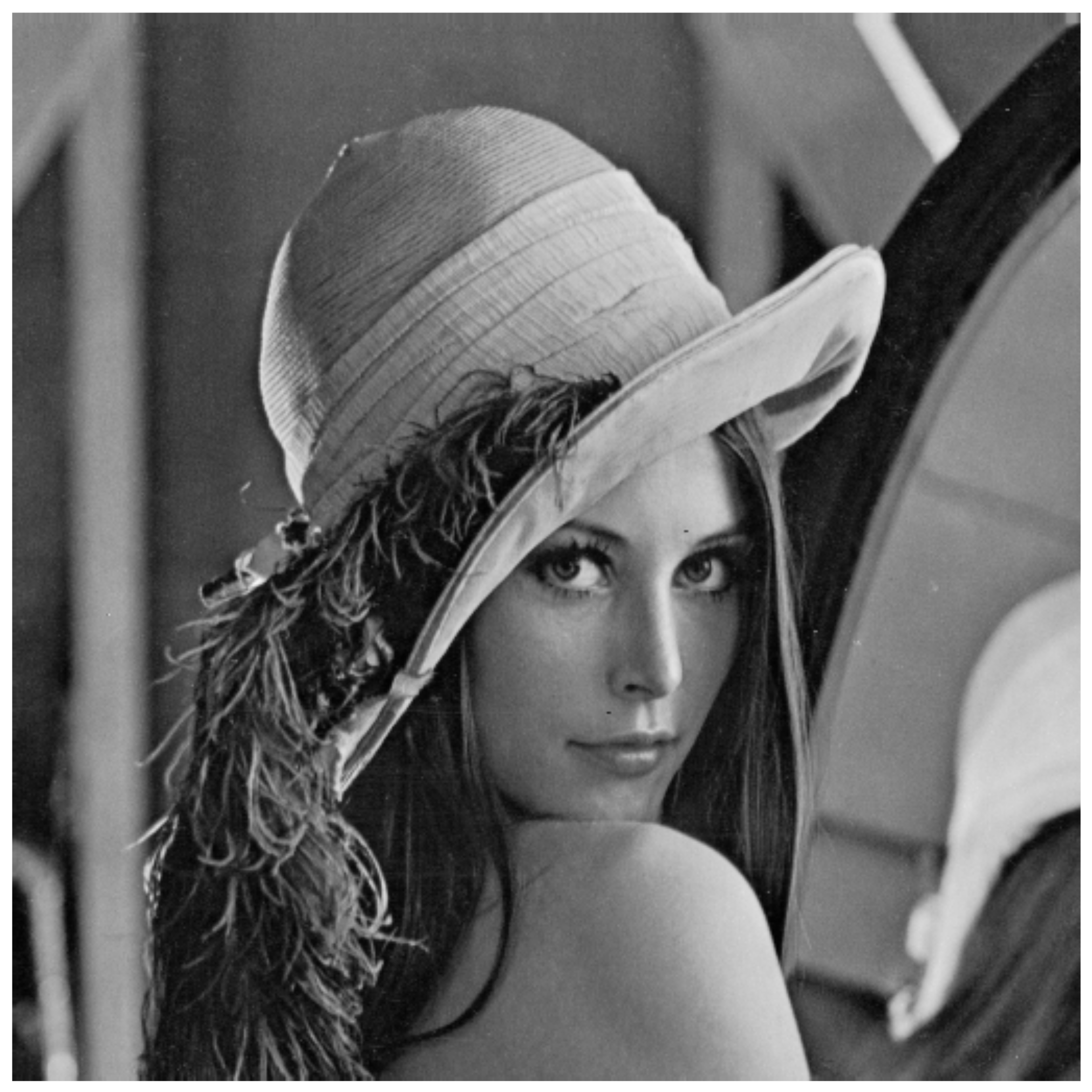
We have performed the compression algorithm based on the DCT, using the Lena.bmp image [2], which has $256\times 256$ pixels and 256 levels of grey; it is represented in the Figure 4.

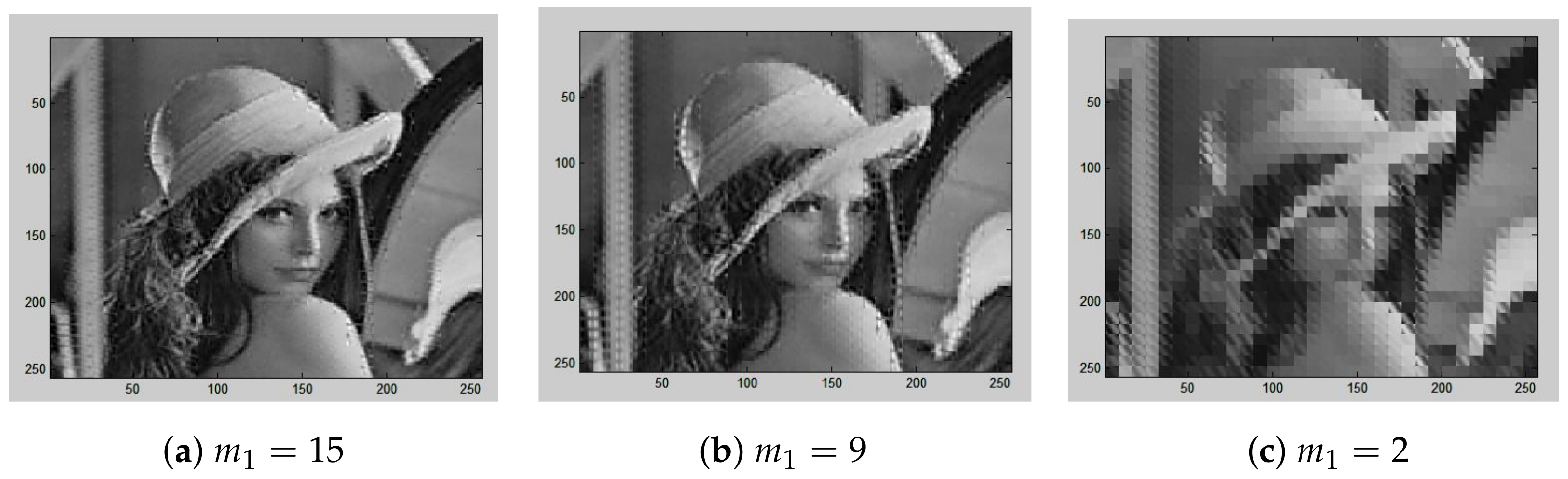
The

Table 2. Experimental results achieved by implementing the DCT compression algorithm.

Number of the Retained Coefficients	Performances of the DCT	Compression lgorithm
	PSNR	MSE
$m_1=15$	27.6054	10.6232
$m_1=9$	25.3436	13.7836
$m_1=2$	21.2242	22.1477

and Figure 5 display the experimental results obtained by implementing the DCT compression algorithm, in Matlab.

Algorithm 1: DCT compression algorithm.

Step 1  Split the initial image into $8\times 8$ pixel blocks (1024 image blocks). Step 2  Process each block by applying the DCT, using relation (8). Step 3  The first nine coefficients for each transformed block are retained in a zigzag fashion and the rest of ($64-9$) the coefficients are cancelled (by making them equal to 0). This stage is illustrated in Figure 6. Step 4  The inverse DCT is applied for each of the 1024 blocks resulted in the previous step. Step 5  The compressed image represented by the matrix $\widehat{X}={\left({\widehat{x}}_{ij}\right)}_{i,j=\overline{1,256}}$ is achieved, where ${\widehat{x}}_{ij}$ denotes the encoded pixel values. Then, the pixel values are converted into integer values. Step 6  The performances of the DCT compression algorithm is evaluated in terms of the Peak Signal-to-Noise Ratio (PSNR), given by [34,35]: $$PSNR=20{log}_{10}\frac{255}{\sqrt{MSE}},$$ (10) where the Mean Squared Error (MSE) is defined as follows [34,35]: $$MSE=\frac{1}{N\times N}\sum _{i=1}^N\sum _{j=1}^N{(x_{ij}-{\widehat{x}}_{ij})}^2,$$ (11) where $N\times N$ means the total number of pixels in the image (in our case $N=256$).

Figure 5. Visual evaluation of the performances corresponding to the DCT compression algorithm.

Figure 5. Visual evaluation of the performances corresponding to the DCT compression algorithm.

Figure 6. Zigzag fashion to retain the first nine coefficients.

Figure 6. Zigzag fashion to retain the first nine coefficients.

4. Fourier Descriptors

The descriptors of different objects can be compared for achieving [36] a measurement of their similarity [2].

The Fourier descriptors [37,38] show interesting properties in terms of the shape of an object, by considering its boundaries.

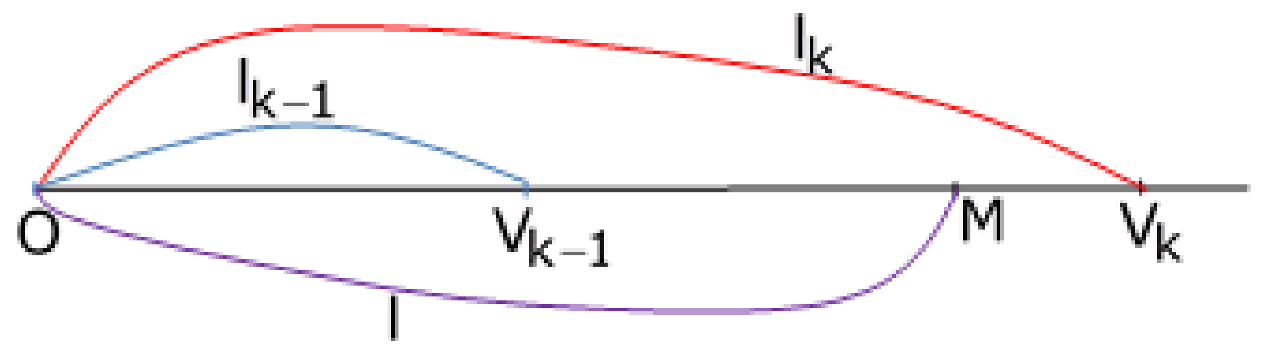
Let $\gamma$ be [2,35] a closed pattern, oriented counterclockwise, described by the parametric representation: $z\left(l\right)=\left(x\right(l),y(l\left)\right)$, where l denotes the length of a circular arc, along the curve $\gamma$, starting from an origin and $0\le l<L$, where L means the length of the boundary.

A point lying on the boundary generates the complex function $u\left(l\right)=x\left(l\right)+\mathrm{i}y\left(l\right)$. We note that $u\left(l\right)$ is a periodic function, with period L.

Definition 2.

The Fourier descriptors are the coefficients associated to the decomposition of the function $u\left(l\right)$ in a complex Fourier series.

By using a similar approach of implementing a Fourier series for building a specific time signal, which consists of cosine/sine waves of different amplitude and frequency, “the Fourier descriptor method uses a series of circles with different sizes and frequencies to build up a two dimensional plot of a boundary” [36] corresponding to an object.

The Fourier descriptors are computed using the formula [2,35]:

$$a_n=\frac{1}{L}{\int }_0^{L}u\left(l\right){\mathrm{e}}^{-\mathrm{i}\frac{2\pi }{L}nl}\mathrm{d}l$$

(12)

such that

$$u\left(l\right)=\sum _{n=-\infty }^{\infty }{a}_n·{\mathrm{e}}^{\mathrm{i}\frac{2\pi }{L}nl}.$$

(13)

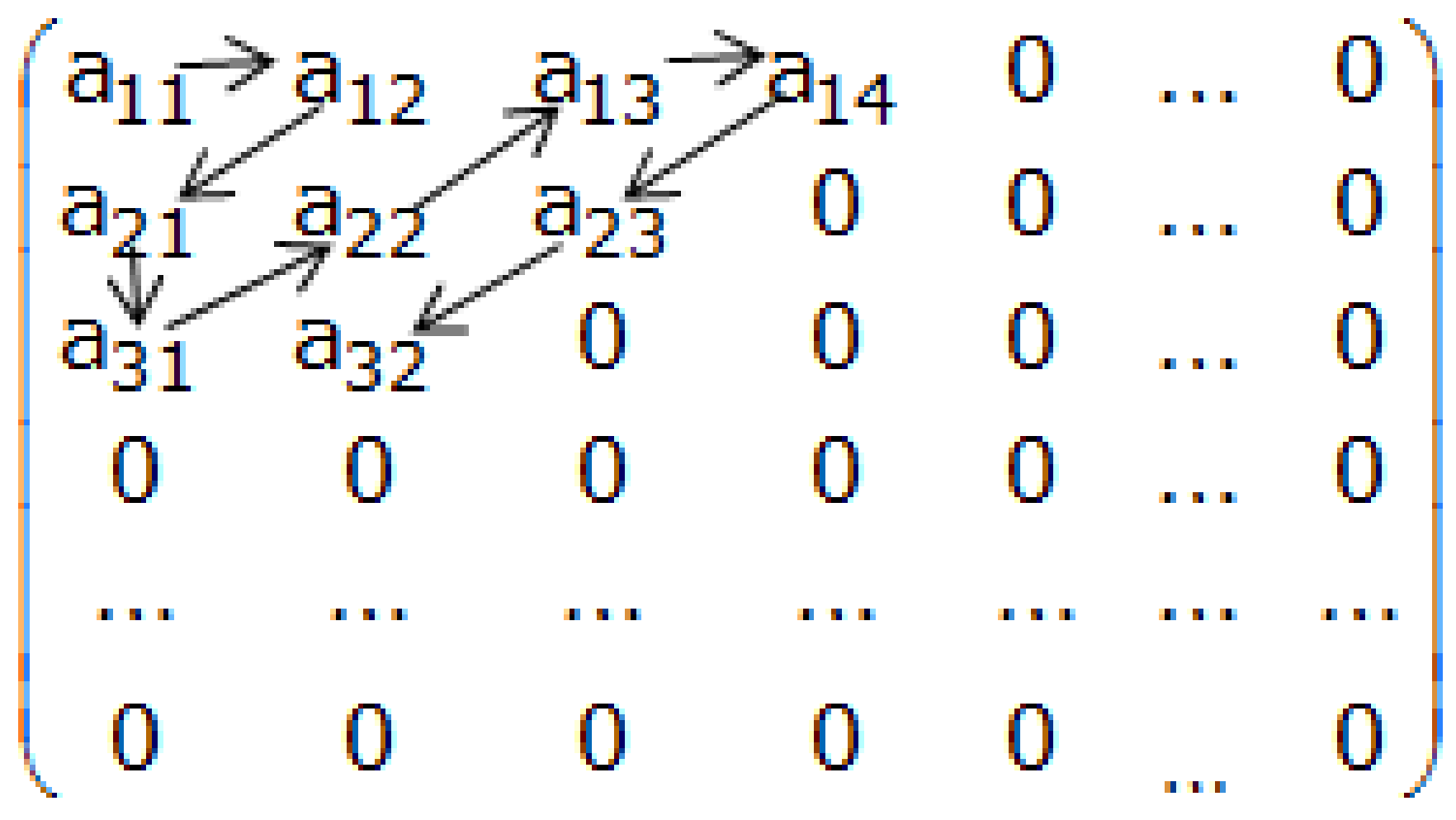
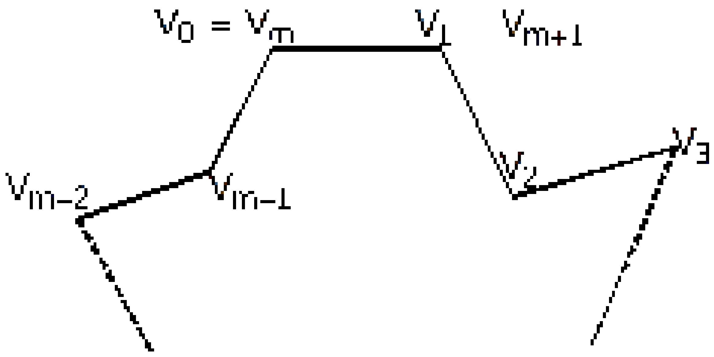
In the case of a polygonal contour, depicted in the Figure 7, we will derive [2,35] an equivalent formula to (12).

Denoting

$$\lambda =\frac{\parallel \overline{V_{k-1}M}\parallel }{\parallel \overline{M{V}_k}\parallel },$$

(14)

namely (see the Figure 8):

$$\lambda =\frac{l-l_{k-1}}{l_k-l},$$

(15)

where $M(x_M,y_M),V_{k-1}(x_{k-1},y_{k-1}),V_k(x_k,y_k)$ and

$$\left\{\begin{array}{c}{l}_0=0,\hfill \\ l_k={\displaystyle \sum _{i=1}^k}|V_i-V_{i-1}|;\end{array}\right.$$

(16)

from (12) it results:

$$a_n=\frac{1}{L}\sum _{k=1}^m{\int }_{l_{k-1}}^{l_k}(x_M\left(l\right)+\mathrm{i}{y}_M\left(l\right))·{\mathrm{e}}^{-\mathrm{i}\frac{2\pi }{L}nl}\mathrm{d}l.$$

(17)

From (14) we deduce:

$$\left\{\begin{array}{c}{x}_M=\frac{x_{k-1}+\lambda x_k}{1+\lambda },\hfill \\ y_M=\frac{y_{k-1}+\lambda y_k}{1+\lambda }.\end{array}\right.$$

(18)

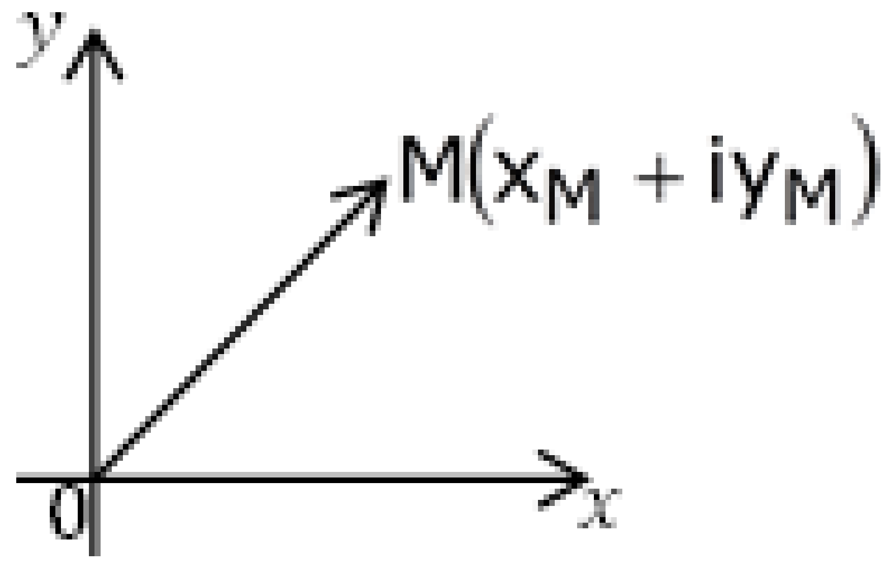
We will regard each coordinate pair as a complex number, as illustrated in the Figure 9:

Taking into consideration the previous assumption and relationships (18) and (15) we get:

$$x_M\left(l\right)+\mathrm{i}{y}_M\left(l\right)=\frac{x_{k-1}+\frac{l-l_{k-1}}{l_k-l}·x_k}{1+\frac{l-l_{k-1}}{l_k-l}}+\mathrm{i}\frac{y_{k-1}+\frac{l-l_{k-1}}{l_k-l}·y_k}{1+\frac{l-l_{k-1}}{l_k-l}}$$

$$=\frac{(x_{k-1}+\mathrm{i}{y}_{k-1})l_k+l[(x_k-x_{k-1})+\mathrm{i}(y_k-y_{k-1})]-(x_k+\mathrm{i}{y}_k)l_{k-1}}{l_k-l_{k-1}}$$

$$=\frac{V_{k-1}{l}_k+l(V_k-V_{k-1})-V_k{l}_{k-1}}{l_k-l_{k-1}};$$

hence, the formula (17) will become:

$$\begin{array}{c}{a}_n=\frac{1}{L}{\displaystyle \sum _{k=1}^m}\frac{1}{l_k-l_{k-1}}{\int }_{l_{k-1}}^{l_k}[V_{k-1}{l}_k+l(V_k-V_{k-1})-V_k{l}_{k-1}]·{\mathrm{e}}^{-\mathrm{i}\frac{2\pi }{L}nl}\mathrm{d}l\\ =\frac{1}{L}{\displaystyle \sum _{k=1}^m}\frac{1}{l_k-l_{k-1}}{\int }_{l_{k-1}}^{l_k}[V_{k-1}{l}_k+l(V_k-V_{k-1})-V_k{l}_{k-1}]·{\mathrm{e}}^{-\mathrm{i}\frac{2\pi }{L}nl}\mathrm{d}l=\end{array}$$

$$a_n=\frac{1}{L}\sum _{k=1}^m\frac{1}{l_k-l_{k-1}}\left[(V_{k-1}{l}_k-V_k{l}_{k-1})·{\int }_{l_{k-1}}^{l_k}{\mathrm{e}}^{-\mathrm{i}\frac{2\pi }{L}nl}\mathrm{d}l+(V_k-V_{k-1})·\underset{I}{\underbrace{{\int }_{l_{k-1}}^{l_k}l·{\mathrm{e}}^{-\mathrm{i}\frac{2\pi }{L}nl}\mathrm{d}l}}\right].$$

(19)

By computing

$$\begin{array}{c}I={\int }_{l_{k-1}}^{l_k}l·{\mathrm{e}}^{-\mathrm{i}\frac{2\pi }{L}nl}\mathrm{d}l=-\frac{1}{\mathrm{i}\frac{2\pi }{L}n}\left(l_k·{\mathrm{e}}^{-\mathrm{i}\frac{2\pi }{L}n{l}_k}-l_{k-1}·{\mathrm{e}}^{-\mathrm{i}\frac{2\pi }{L}n{l}_{k-1}}\right)\\ +\frac{1}{{\left(\frac{2\pi }{L}n\right)}^2}\left({\mathrm{e}}^{-\mathrm{i}\frac{2\pi }{L}n{l}_k}-{\mathrm{e}}^{-\mathrm{i}\frac{2\pi }{L}n{l}_{k-1}}\right)\end{array}$$

and substituting it into (19) we shall achieve:

$$a_n=\frac{1}{L}\sum _{k=1}^m\frac{1}{l_k-l_{k-1}}·T_k,$$

(20)

where

$$\begin{array}{c}{T}_k=-\frac{1}{\mathrm{i}\frac{2\pi }{L}n}(V_{k-1}{l}_k-V_k{l}_{k-1})·\left({\mathrm{e}}^{-\mathrm{i}\frac{2\pi }{L}n{l}_k}-{\mathrm{e}}^{-\mathrm{i}\frac{2\pi }{L}n{l}_{k-1}}\right)\\ -\frac{1}{\mathrm{i}\frac{2\pi }{L}n}(V_k-V_{k-1})·\left(l_k{\mathrm{e}}^{-\mathrm{i}\frac{2\pi }{L}n{l}_k}-l_{k-1}{\mathrm{e}}^{-\mathrm{i}\frac{2\pi }{L}n{l}_{k-1}}\right)\end{array}$$

$$+\frac{1}{{\left(\frac{2\pi }{L}n\right)}^2}(V_k-V_{k-1})·\left({\mathrm{e}}^{-\mathrm{i}\frac{2\pi }{L}n{l}_k}-{\mathrm{e}}^{-\mathrm{i}\frac{2\pi }{L}n{l}_{k-1}}\right),$$

namely

$$\begin{array}{c}{T}_k=-\frac{1}{\mathrm{i}\frac{2\pi }{L}n}\left[V_k(l_k-l_{k-1})·{\mathrm{e}}^{-\mathrm{i}\frac{2\pi }{L}n{l}_k}-V_{k-1}(l_k-l_{k-1})·{\mathrm{e}}^{-\mathrm{i}\frac{2\pi }{L}n{l}_{k-1}}\right]\\ +\frac{1}{{\left(\frac{2\pi }{L}n\right)}^2}(V_k-V_{k-1})·\left({\mathrm{e}}^{-\mathrm{i}\frac{2\pi }{L}n{l}_k}-{\mathrm{e}}^{-\mathrm{i}\frac{2\pi }{L}n{l}_{k-1}}\right).\end{array}$$

(21)

Therefore, on the basis of the relations (21) and (16) from which it results

$$l_k-l_{k-1}=|V_k-V_{k-1}|,(\forall )k=\overline{1,m},$$

the formula (20), which allows us the computation of the Fourier descriptors will be:

$$\begin{array}{c}{a}_n=-\frac{1}{2\pi \mathrm{i}n}{\displaystyle \sum _{k=1}^m}\left(V_k·{\mathrm{e}}^{-\mathrm{i}\frac{2\pi }{L}n{l}_k}-V_{k-1}·{\mathrm{e}}^{-\mathrm{i}\frac{2\pi }{L}n{l}_{k-1}}\right)\\ +\frac{L}{{\left(2\pi n\right)}^2}{\displaystyle \sum _{k=1}^m}\frac{V_k-V_{k-1}}{|V_k-V_{k-1}|}·\left({\mathrm{e}}^{-\mathrm{i}\frac{2\pi }{L}n{l}_k}-{\mathrm{e}}^{-\mathrm{i}\frac{2\pi }{L}n{l}_{k-1}}\right).\end{array}$$

(22)

The principal advantages of the Fourier Descriptor method for object recognition consists in the invariance to translation, rotation and scale displayed by the Fourier descriptors are [36].

5. Measuring Image Information

5.1. Entropy and Information

The fundamental premise in Information Theory is that the information generation can be modeled like a probabilistic process [39,40,41,42,43,44,45,46,47]

Hence, an event E, which occurs with probability $P\left(E\right)$ will contain $I\left(E\right)$ information units, where [11]:

$$I\left(E\right)=log\frac{1}{P\left(E\right)}=-logP\left(E\right).$$

There is the convention that the basis of the logarithm determines the unit used to measure the information. In the case when the basis is equal with two, then the information unit it is called a bit (binary digit).

Assuming a discrete set of symbols $\{a_1,\dots ,a_m\}$, having the associated probabilities $\{P\left(a_1\right),\dots ,P\left(a_m\right)\}$ we see that the entropy of the discrete distribution is [11]:

$$H\left(z\right)=-\sum _{j=1}^{m}P\left(a_j\right)logP\left(a_j\right),$$

(23)

where $z={(P\left(a_1\right),\dots ,P\left(a_m\right))}^t$.

We can note that the entropy from the Equation (23) just depends on the probabilities of the symbols and it measures the randomness or unpredictability of the respective symbols drawn from a given sequence; in fact, the entropy defines the average amount of information that can be obtained by observing a single output of a primary source.

The information which is transferred to the receiver through an information transmission system is a random discrete set of symbols $\{b_1,\dots ,b_n\}$ too, with the corresponding probabilities $\{P\left(b_1\right),\dots ,P\left(b_n\right)\}$, where [11]:

$$P\left(b_k\right)=\sum _{j=1}^{m}P\left(b_k\right|a_j)·P\left(a_j\right),(\forall )k=\overline{1,n}.$$

(24)

The Equation (24) can be written in the matrix form [11]:

$$v=Qz,$$

(25)

where

• $v={(P\left(b_1\right),\dots ,P\left(b_n\right))}^t$ is the probability distribution of the output alphabet $\{b_1,\dots ,b_n\}$;
• the matrix $Q={\left(q_{k,j}\right)}_{\begin{array}{c}1\le k\le n\\ 1\le j\le m\end{array}}$ means is associated with the information transmission system:

  $$Q=\left(\begin{array}{cccc}P\left(b_1\right|a_1)& P\left(b_1\right|a_2)& \dots & P\left(b_1\right|a_m)\\ P\left(b_2\right|a_1)& P\left(b_2\right|a_2)& \dots & P\left(b_2\right|a_m)\\ ⋮& ⋮& ⋮& ⋮\\ P\left(b_n\right|a_1)& P\left(b_n\right|a_2)& \dots & P\left(b_n\right|a_m)\end{array}\right),$$

  (26)

  where

  $$q_{k,j}=P\left(b_k\right|a_j),(\forall )j=\overline{1,m},k=\overline{1,n}.$$

One can define [11]:

(1)

the conditional entropy:

$$H\left(z\right|v)=-\sum _{j=1}^m\sum _{k=1}^{n}P(a_j,b_k)logP\left(a_j\right|b_k),$$

(27)

where $P(a_j,b_k)$ means the joint probability, namely the probability of $b_k$ occurring at the same time that $a_j$ occurs:

$$P(a_j,b_k)=P\left(b_k\right)·P\left(a_j\right|b_k).$$

(28)

(2)

the mutual information between z and v, which expresses the reduction of uncertainty about z because of the knowledge of v:

$$I(z;v)=H\left(z\right)-H\left(z\right|v),$$

(29)

namely

$$I(z;v)=-\sum _{j=1}^{m}P\left(a_j\right)logP\left(a_j\right)+\sum _{j=1}^m\sum _{k=1}^{n}P(a_j,b_k)logP\left(a_j\right|b_k)=$$

$$=-\sum _{j=1}^m\sum _{k=1}^{n}P(a_j,b_k)logP\left(a_j\right)+\sum _{j=1}^m\sum _{k=1}^{n}P(a_j,b_k)logP\left(a_j\right|b_k)=$$

$$=-\sum _{j=1}^m\sum _{k=1}^{n}P(a_j,b_k)\left[logP\left(a_j\right)-logP\left(a_j\right|b_k)\right]=$$

$$=\sum _{j=1}^m\sum _{k=1}^{n}P(a_j,b_k)log\frac{P\left(a_j\right|b_k)}{P\left(a_j\right)};$$

therefore

$$I(z;v)=\sum _{j=1}^m\sum _{k=1}^{n}P(a_j,b_k)log\frac{P(a_j,b_k)}{P\left(a_j\right)·P\left(b_k\right)}.$$

(30)

Taking into account the Bayes Rule [48]:

$$P(a_j,b_k)=P\left(a_j\right)·P\left(b_k\right|a_j)=P\left(b_k\right)·P\left(a_j\right|b_k)$$

and from the Equation (24) it will result that:

$$I(z;v)=\sum _{j=1}^m\sum _{k=1}^{n}P\left(a_j\right)·q_{kj}log\frac{q_{kj}}{{\displaystyle \sum _{j=1}^m}P\left(a_j\right)q_{kj}}.$$

(31)

From the Equation (30) we can deduce that the minimum value of $I(z;v)$ is 0 and can be achieved in the case when the input and the output alphabet are mutually independent [48], i.e.,

$$P(a_j,b_k)=P\left(a_j\right)·P\left(b_k\right).$$

5.2. The Case of the Binary Information Sources

Let a binary information source with the source alphabet $A=\{a_1,a_2\}=\{0,1\}$ and let $P\left(a_1\right),P\left(a_2\right)$ be the probabilities that the source to produce the symbols $a_1$ and $a_2$, such that [11]:

$$P\left(a_1\right)=p_{bs}$$

(32)

$$P\left(a_2\right)=1-p_{bs}={\overline{p}}_{bs}.$$

(33)

By using the Equation (23) it will result that the following entropy of the binary source [11]:

$$H\left(z\right)=-p_{bs}{log}_2{p}_{bs}-(1-p_{bs}){log}_2(1-p_{bs}),$$

where $z={(p_{bs},1-p_{bs})}^t$, i.e., one achieves the binary entropy function [11]:

$$H\left(z\right)=-p_{bs}{log}_2{p}_{bs}-{\overline{p}}_{bs}{log}_2{\overline{p}}_{bs},$$

(34)

having its maximum value (of 1 bit) when $p_{bs}=\frac{1}{2}$.

If there is some noise during the data transmission then the matrix Q from the Equation (26) can be defined as [11]:

$$Q=\left(\begin{array}{cc}1-p_e& p_e\\ p_e& 1-p_e\end{array}\right)=\left(\begin{array}{cc}{\overline{p}}_e& p_e\\ p_e& {\overline{p}}_e\end{array}\right),$$

(35)

$p_e$ being the probability of an error during the transmission of any symbol.

In the case when the output alphabet delivered at the receiver is the the set of symbols $B=\{b_1,b_2\}=\{0,1\}$ one achieves that [11]:

$$v=\left(\begin{array}{c}{\overline{p}}_{bs}{p}_{bs}+p_e{\overline{p}}_{bs}\\ p_e{p}_{bs}+{\overline{p}}_e{\overline{p}}_{bs}\end{array}\right),$$

(36)

i.e., one can compute:

$$P\left(b_1\right)={\overline{p}}_e{p}_{bs}+p_e{\overline{p}}_{bs}$$

(37)

$$P\left(b_2\right)=p_e{p}_{bs}+{\overline{p}}_e{\overline{p}}_{bs}.$$

(38)

Hence, on the basis of the formula (31), the mutual information between z and v will be:

$$\begin{array}{c}I(z;v)=p_{bs}{\overline{p}}_e{log}_2\frac{{\overline{p}}_e}{{\overline{p}}_e{p}_{bs}+p_e{\overline{p}}_{bs}}+p_{bs}{p}_e{log}_2\frac{p_e}{p_e{p}_{bs}+{\overline{p}}_e{\overline{p}}_{bs}}+\\ +{\overline{p}}_{bs}{p}_e{log}_2\frac{p_e}{{\overline{p}}_e{p}_{bs}+p_e{\overline{p}}_{bs}}+{\overline{p}}_e{\overline{p}}_{bs}{log}_2\frac{{\overline{p}}_e}{p_e{p}_{bs}+{\overline{p}}_e{\overline{p}}_{bs}}=\\ =-(p_{bs}{\overline{p}}_e+{\overline{p}}_{bs}{p}_e){log}_2({\overline{p}}_e{p}_{bs}+p_e{\overline{p}}_{bs})-(p_{bs}{p}_e+{\overline{p}}_e{\overline{p}}_{bs}){log}_2(p_{bs}{p}_e+{\overline{p}}_e{\overline{p}}_{bs})+\\ +{\overline{p}}_e(p_{bs}+{\overline{p}}_{bs}){log}_2{\overline{p}}_e+p_e(p_{bs}+{\overline{p}}_{bs}){log}_2{p}_e;\end{array}$$

therefore [11]:

$$I(z;v)=H_{bs}(p_{bs}{p}_e+{\overline{p}}_e{\overline{p}}_{bs})-H_{bs}\left(p_e\right).$$

(39)

From the Equation (39) one can notice that:

• $I(z;v)=0$ when $p_{bs}$ has the value 0 or 1;
• the maximum value of $I(z;v)$ is $C=1-H_{bs}\left(p_e\right)$ (it means the maximum amount of information that can be transferred, i.e., the capacity of the binary transmission system = BST) and can be achieved when the symbols of the binary source are equally likely to occur, namely $p_{bs}=\frac{1}{2}$. For $p_e=1$ one obtains the maximum capacity of the BST: $C=1-H_{bs}=1$, while for $p_e=1/2$ one deduces that $C=0$, i.e., any information can not be transferred through the BST.

5.3. The Noiseless Coding Theorem

Let be a zero-memory source $(A,z)$, from the Equation (23), which is an information source, having only statistically independent symbols. We suppose that the output of this source is a n- tuple of symbols, then the output of the given zero-memory source is the set $A^{\prime }=\{{\alpha }_1,\dots ,{\alpha }_{m^n}\}$ has $m^n$ possible values ${\alpha }_i$, each of them consisting in n symbols from the alphabet A.

As there are the inequalities [11]:

$$log\frac{1}{P\left({\alpha }_i\right)}\le l\left({\alpha }_i\right)<log\frac{1}{P\left({\alpha }_i\right)}+1,$$

(40)

where $l\left({\alpha }_i\right)$, introduced by the Equation (5) is the length of the coding word used to represent ${\alpha }_i$, one achieves:

$$\sum _{i=1}^{m^n}P\left({\alpha }_i\right)log\frac{1}{P\left({\alpha }_i\right)}\le \sum _{i=1}^{m^n}P\left({\alpha }_i\right)l\left({\alpha }_i\right)<\sum _{i=1}^{m^n}P\left({\alpha }_i\right)log\frac{1}{P\left({\alpha }_i\right)}+1;$$

(41)

therefore [11]:

$$H\left(z^{\prime }\right)\le L_{avg}^{\prime }<H\left(z^{\prime }\right)+1,$$

(42)

where $L_{avg}^{\prime }$ means the average number of code symbols required to represent all n-symbol groups.

From the Equation (42) one deduces the Shannon’s first theorem (the noiseless coding theorem) [11], which claims that the output of a zero-memory source can be represented with an average of $H\left(z\right)$ information units per source symbol:

$$\frac{H\left(z^{\prime }\right)}{n}\le \frac{L_{avg}^{\prime }}{n}<\frac{H\left(z^{\prime }\right)}{n}+\frac{1}{n},$$

(43)

namely:

$$H\left(z\right)\le \frac{L_{avg}^{\prime }}{n}<H\left(z\right)+\frac{1}{n}$$

(44)

or:

$$\underset{n\to \infty }{lim}\frac{L_{avg}^{\prime }}{n}=H\left(z\right).$$

(45)

The Equation (45) proves that the expression $\frac{L_{avg}^{\prime }}{n}$ can be approximated with $H\left(z\right)$ by encoding infinitely long extensions corresponding to the single-symbol source.

The efficiency of the coding strategy is given by [11]:

$$\eta =n·\frac{H\left(z\right)}{L_{avg}^{\prime }}.$$

(46)

6. Huffman Coding

Huffman Coding [11] is an error-free compression method, designed to remove the coding redundancy, by yielding the smallest number of code symbols per source symbol, which in practice can be represented by the intensities of an image or the output of a mapping operation.

The Huffman algorithm finds the optimal code for an alphabet of symbols, taking into account the condition that the probabilities associated with the symbols have to be coded one at a time.

The approach of Huffman consists in following:

Step 1 

Approximate the given data with a Poisson distribution to avoid the undefined entropies.

Step 2 

Create a series of source reductions by sorting the probabilities of the respective symbols in a descending order in order to combine the lowest probability symbols into a single symbol, which replace them in the next source reduction. This process can be repeated as long as a source with two symbols is not reached.

Step 3 

Code each reduced source, by starting with the smallest source and then go back to the original source of this work, taking into account that the symbols 0 and 1 are the binary codes with minimal length for a two-symbol source.

The Huffman coding efficiency can be computed using the formula [11]:

$$\eta =\frac{L_{avg}}{H\left(z\right)},$$

(47)

$L_{avg}$ being the average length of the code words, defined in the relation (5) and $H\left(z\right)$ being the entropy of the discrete distribution, introduced by the Equation (23).

7. Experimental Evaluation

7.1. Data Sets

We will use [2] the images from the PASCAL dataset for evaluating the performance of our method using Matlab.

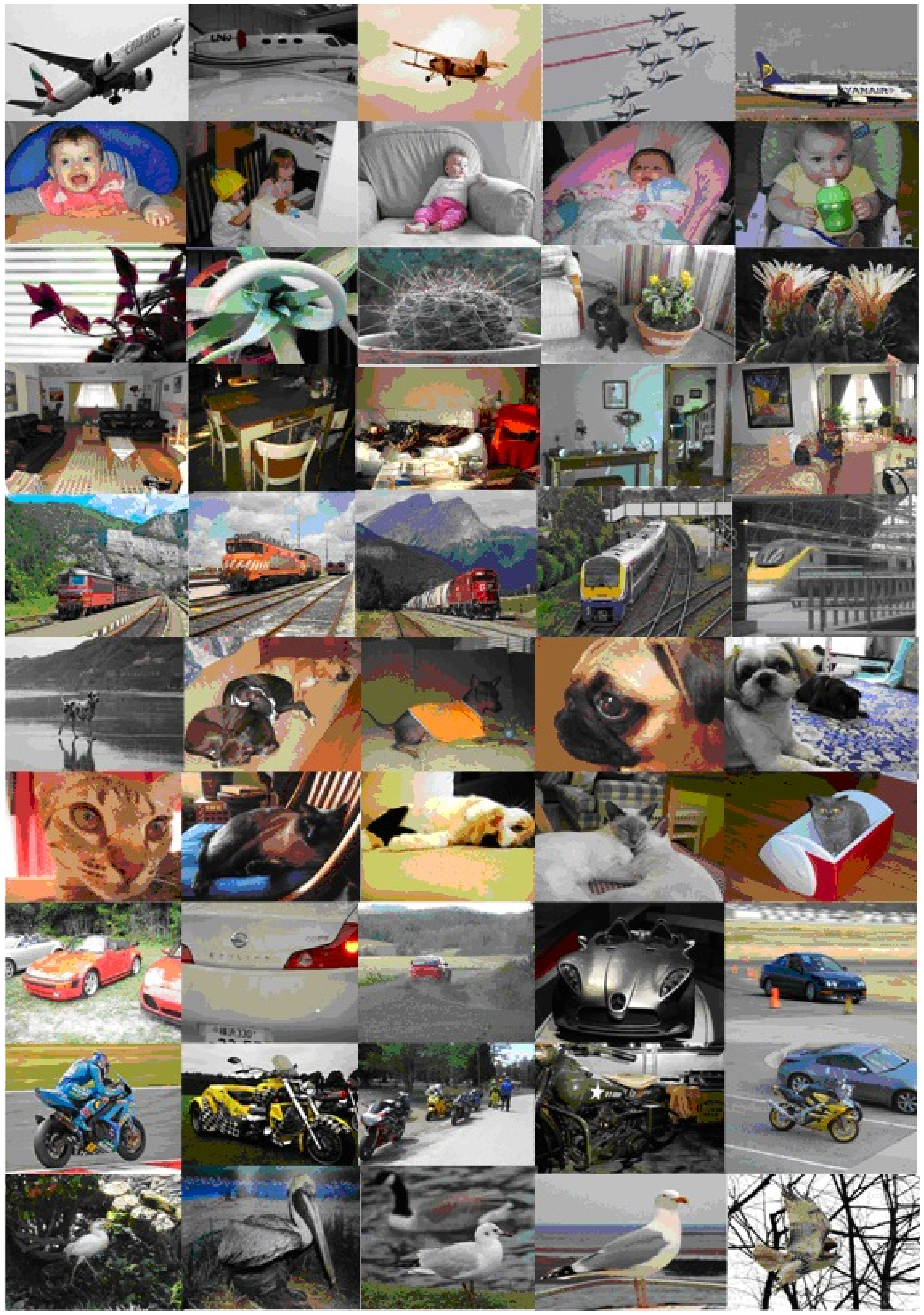
In this paper we have used 10,102 images from the VOC data sets, which contain significant variability in terms of object size, orientation, pose, illumination, position and occlusion.

The database consists of 20 object classes: aeroplane, bicycle, bird, boat, bottle, bus, car, motorbike, train, sofa, table, chair, tv/monitor, potted plant, person, cat, cow, dog, horse and sheep.

We have used The ColorDescriptor engine [49] for extracting the image descriptors from all the images.

The Figure 10 shows 50 images from the VOC data base.

The performance of our method has been assessed using images from the PASCAL dataset The Pascal VOC challenge represents [34] a benchmark in visual object category recognition and detection, as it provides the vision and machine learning communities with a standard data set of images and annotation.

Our approach uses 64 descriptors for each image belonging to the training and test set, therefore the number of symbols is 64.

7.2. Experimental Results

For our experiments, we used the descriptors corresponding to some images from the VOC data sets and after we approximated our data with a Poisson distribution, we computed the image entropy, the average length of the code words and the Huffman coding efficiency too. We have applied the following Algorithm:

Step 1 

Approximate the given data with a Poisson distribution.

Step 2 

Create a series of source reductions by sorting the probabilities of the respective symbols in a descending order in order to combine the lowest probability symbols into a single symbol, which replace them in the next source reduction. This process can be repeated as long as a source with two symbols is not reached.

Step 3 

Code each reduced source, by starting with the smallest source and then go back the original source of this work, taking into account that the symbols 0 and 1 are the binary codes with minimal length for a two-symbol source.

The achieved results are illustrated in the

Table 3. The Huffman coding efficiency.

Image	Entropy	${\mathit{L}}_{\mathit{avg}}$	Coding Efficiency
	4.6324	4.6534	0.9955
	4.5401	4.5609	0.9955
	4.5802	4.6005	0.9955
	4.6037	4.6233	0.9957
	4.5277	4.5461	0.9959

,

Table 4. The Huffman coding efficiency.

Image	Entropy	${\mathit{L}}_{\mathit{avg}}$	Coding Efficiency
	4.5839	4.6039	0.9957
	4.5681	4.5869	0.9959
	4.4587	4.4823	0.9947
	4.5221	4.5411	0.9958
	4.4257	4.4527	0.9939

,

Table 5. The Huffman coding efficiency.

Image	Entropy	${\mathit{L}}_{\mathit{avg}}$	Coding Efficiency
	4.5509	4.5693	0.9959
	4.5737	4.5927	0.9958
	4.5484	4.5668	0.9959
	4.4696	4.4928	0.9948
	4.5567	4.5766	0.9956

,

Table 6. The Huffman coding efficiency.

Image	Entropy	${\mathit{L}}_{\mathit{avg}}$	Coding Efficiency
	4.462	4.4856	0.9947
	4.5742	4.5934	0.9958
	4.4407	4.4647	0.9946
	4.5362	4.5563	0.9956
	4.4566	4.4799	0.9948

,

Table 7. The Huffman coding efficiency.

Image	Entropy	${\mathit{L}}_{\mathit{avg}}$	Coding Efficiency
	4.5156	4.5368	0.9953
	4.6350	4.6559	0.9955
	4.6124	4.6331	0.9955
	4.4597	4.4833	0.9947
	4.4924	4.515	0.9949

,

Table 8. The Huffman coding efficiency.

Image	Entropy	${\mathit{L}}_{\mathit{avg}}$	Coding Efficiency
	4.4930	4.5153	0.9951
	4.5541	4.5732	0.9958
	4.5026	4.5219	0.9957
	4.5691	4.5877	0.9959
	4.541	4.5612	0.9955

,

Table 9. The Huffman coding efficiency.

Image	Entropy	${\mathit{L}}_{\mathit{avg}}$	Coding Efficiency
	4.5233	4.5422	0.9958
	4.3961	4.4247	0.9935
	4.6318	4.6529	0.9954
	4.5837	4.6037	0.9957
	4.5661	4.5853	0.9958

,

Table 10. The Huffman coding efficiency.

Image	Entropy	${\mathit{L}}_{\mathit{avg}}$	Coding Efficiency
	4.5921	4.6115	0.9957
	4.6093	4.6299	0.9955
	4.5063	4.5257	0.9957
	4.5116	4.5322	0.9954
	4.5825	4.6025	0.9957

and

Table 11. The Huffman coding efficiency.

Image	Entropy	${\mathit{L}}_{\mathit{avg}}$	Coding Efficiency
	4.3554	4.3880	0.9926
	4.5911	4.6105	0.9958
	4.4944	4.5159	0.9952
	4.4516	4.4752	0.9947
	4.3646	4.3958	0.9929

.

8. Conclusions

This paper proposes to improve the Huffman coding efficiency by adjusting the data using a Poisson distribution, which avoids the undefined entropies too. The performance of our method has been assessed in Matlab, by using a set of images from the PASCAL dataset.

The scientific value added of our paper consists in applying the Poisson distribution in order to minimize the average length of the Huffman code words.

The PASCAL VOC challenge represents [34] a benchmark in visual object category recognition and detection as it provides the vision and machine learning communities with a standard data set of images and annotation.

In this paper we have used 10,102 images from the VOC data sets, which contain significant variability in terms of object size, orientation, pose, illumination, position and occlusion.

The database consists of 20 object classes: aeroplane, bicycle, bird, boat, bottle, bus, car, motorbike, train, sofa, table, chair, tv/monitor, potted plant, person, cat, cow, dog, horse and sheep.

The data of our information source are different from a finite memory source (Markov), where its output depends on a finite number of previous outputs.

References

- Zaka, B. Theory and Applications of Similarity Detection Techniques. 2009. Available online: http://www.iicm.tugraz.at/thesis/bilal_dissertation.pdf (accessed on 14 July 2022).
- Iatan, I.F. Issues in the Use of Neural Networks in Information Retrieval; Springer: Cham, Switzerland, 2017. [Google Scholar]
- Hwang, C.M.; Yang, M.S.; Hung, W.L.; Lee, M.L. A similarity measure of intuitionistic fuzzy sets based on the Sugeno integral with its application to pattern recognition. Inf. Sci. 2012, 189, 93–109. [Google Scholar] [CrossRef]
- Chen, Y.; Garcia, E.K.; Gupta, M.R.; Rahimi, A.; Cazzanti, L. Similarity-based Classification: Concepts and Algorithms. J. Mach. Learn. Res. 2009, 10, 747–776. [Google Scholar]
- Suzuki, K.; Yamada, H.; Hashimoto, S. A similarity-based neural network for facial expression analysis. Pattern Recognit. Lett. 2007, 28, 1104–1111. [Google Scholar] [CrossRef]
- Duda, D.O.; Hart, P.E.; Stork, D.G. Pattern Classification, 2nd ed.; John Wiley: New York, NY, USA, 2001. [Google Scholar]
- Andersson, J. Statistical Analysis with Swift; Apress: New York, NY, USA, 2021. [Google Scholar]
- Reshadat, V.; Feizi-Derakhshi, M.R. Neural network-based methods in information retrieval. Am. J. Sci. Res. 2012, 58, 33–43. [Google Scholar]
- Cai, F.; China, C.; de Rijke, M. A Survey of Query Auto Completion in Information Retrieval. Found. Trends R Signal Process. 2016, 10, 273–363. [Google Scholar]
- Liu, B. Web DataMining; Springer: Berlin/Heidelberg, Germany, 2008. [Google Scholar]
- Gonzalez, R.C.; Woods, R.E. Digital Image Processing, 4th ed.; Pearson: New York, NY, USA, 2018. [Google Scholar]
- Burgerr, W.; Burge, M.J. Principles of Digital Image Processing; Fundamental Techniques; Springer: London, UK, 2009. [Google Scholar]
- Webb, A. Statistical Pattern Recognition, 2nd ed.; John Wiley and Sons: New York, NY, USA, 2002. [Google Scholar]
- Kreyszig, E. Advanced Engineering Mathematics; John Wiley and Sons: New York, NY, USA, 2006. [Google Scholar]
- Trandafir, R.; Iatan, I.F. Modelling and Simulation: Theoretical Notions and Applications; Conspress: Bucharest, Romania, 2013. [Google Scholar]
- Anastassiou, G.; Iatan, I. Modern Algorithms of Simulation for Getting Some Random Numbers. J. Comput. Anal. Appl. 2013, 15, 1211–1222. [Google Scholar]
- Iatan, I.F.; Trandafir, R. Validating in Matlab of some Algorithms to Simulate some Continuous and Discrete Random Variables. In Proceedings of the Mathematics and Educational Symposium of Department of Mathematics and Computer Science; Technical University of Civil Engineering Bucharest: București, Romania; MatrixRom: Bucharest, Romania, 2014; pp. 67–72. [Google Scholar]
- Kumar, P.; Parmar, A. Versatile Approaches for Medical Image Compression. Procedia Comput. Sci. 2020, 167, 1380–1389. [Google Scholar] [CrossRef]
- Wilhelmsson, D.; Mikkelsen, L.P.; Fæster, S.; Asp, L.E. X-ray tomography data of compression tested unidirectional fibre composites with different off-axis angles. Data Brief 2019, 25, 104263. [Google Scholar] [CrossRef]
- Wu, F.Y.; Yang, K.; Sheng, X. Optimized compression and recovery of electrocardiographic signal for IoT platform. Appl. Soft Comput. J. 2020, 96, 106659. [Google Scholar] [CrossRef]
- Norris, D.; Kalm, K. Chunking and data compression in verbal short-term memory. Cognition 2021, 208, 104534. [Google Scholar] [CrossRef]
- Peralta, M.; Jannin, P.; Haegelen, C.; Baxter, J.S.H. Data imputation and compression for Parkinson’s disease clinical questionnaires. Artif. Intell. Med. 2021, 114, 102051. [Google Scholar] [CrossRef]
- Calderoni, L.; Magnani, A. The impact of face image compression in future generation electronic identity documents. Forensic Sci. Int. Digit. Investig. 2022, 40, 301345. [Google Scholar] [CrossRef]
- Coutinho, V.A.; Cintra, R.J.; Bayer, F.B. Low-complexity three-dimensional discrete Hartley transform approximations for medical image compression. Comput. Biol. Med. 2021, 139, 3105018. [Google Scholar] [CrossRef]
- Ettaouil, M.; Ghanou, Y.; El Moutaouakil, K.; Lazaar, M. Image Medical Compression by a new Architecture Optimization Model for the Kohonen Networks. Int. J. Comput. Theory Eng. 2011, 3, 204–210. [Google Scholar] [CrossRef]
- Dokuchaev, N.G. On Data Compression and Recovery for Sequences Using Constraints on the Spectrum Range. Probl. Inf. Transm. 2021, 57, 368–372. [Google Scholar] [CrossRef]
- Du, Y.; Yu, H. Medical Data Compression and Sharing Technology Based on Blockchain. In International Conference on Algorithmic Applications in Management; Lecture Notes in Computer Science Book Series (LNTCS); Springer: Cham, Switzerland, 2020; Volume 12290, pp. 581–592. [Google Scholar]
- Ishikawa, M.; Kawakami, H. Compression-based distance between string data and its application to literary work classification based on authorship. Comput. Stat. 2013, 28, 851–878. [Google Scholar] [CrossRef]
- Jha, C.K.; Kolekar, M.H. Electrocardiogram data compression using DCT based discrete orthogonal Stockwell transform. Biomed. Signal Process. Control 2018, 46, 174–181. [Google Scholar] [CrossRef]
- Netravali, A.N.; Haskell, B.G. Digital Pictures: Representation and Compression; Springer: Cham, Switzerland, 2012. [Google Scholar]
- Vlaicu, A. Digital Image Processing; Microinformatica Group: Cluj-Napoca, Romania, 1997. (In Romanian) [Google Scholar]
- Shih, F.Y. Image Processing and Pattern Recognition; Fundamentals and Techniques; John Wiley and Sons: New York, NY, USA, 2010. [Google Scholar]
- Tuduce, R.A. Signal Theory; Bren: Bucharest, Romania, 1998. [Google Scholar]
- Everingham, M.; Van Gool, L.; Williams, C.K.I.; Winn, J.; Zisserman, A. A Fuzzy Neural Network and its Application to Pattern Recognition. IEEE Trans. Fuzzy Syst. 2010, 88, 303–338. [Google Scholar]
- Neagoe, V.E.; Stǎnǎşilǎ, O. Pattern Recognition and Neural Networks; Matrix Rom: Bucharest, Romania, 1999. (In Romanian) [Google Scholar]
- Janse van Rensburg, F.J.; Treurnicht, J.; Fourie, C.J. The Use of Fourier Descriptors for Object Recogntion in Robotic Assembly. In Proceedings of the 5th CIRP International Seminar on Intelligent Computation in Manufacturing Engineering, Ischia, Italy, 25–28 July 2006. [Google Scholar]
- Yang, C.; Yu, Q. Multiscale Fourier descriptor based on triangular features for shape retrieval. Signal Process. Image Commun. 2019, 71, 110–119. [Google Scholar] [CrossRef]
- De, P.; Ghoshal, D. Recognition of Non Circular Iris Pattern of the Goat by Structural, Statistical and Fourier Descriptors. Procedia Comput. Sci. 2016, 89, 845–849. [Google Scholar] [CrossRef] [Green Version]
- Preda, V. Statistical Decision Theory; Romanian Academy: Bucharest, Romania, 1992. [Google Scholar]
- Preda, V.C. The Student distribution and the principle of maximum entropy. Ann. Inst. Stat. Math. 1982, 34, 335–338. [Google Scholar] [CrossRef]
- Preda, V.; Balcau, C.; Niculescu, C. Entropy optimization in phase determination with linear inequality constraints. Rev. Roum. Math. Pures Appl. 2010, 55, 327–340. [Google Scholar]
- Preda, V.; Dedu, S.; Sheraz, M. Second order entropy approach for risk models involving truncation and censoring. Proc. Rom.-Acad. Ser. Math. Phys. Tech. Sci. Inf. Sci. 2016, 17, 195–202. [Google Scholar]
- Preda, V.; Băncescu, I. Evolution of non-stationary processes and some maximum entropy principles. Ann. West Univ.-Timis.-Math. Comput. Sci. 2018, 56, 43–70. [Google Scholar] [CrossRef]
- Barbu, V.S.; Karagrigoriou, A.; Preda, V. Entropy and divergence rates for Markov chains: II. The weighted case. Proc. Rom.-Acad.-Ser. A 2018, 19, 3–10. [Google Scholar]
- Abdul-Sathar, E.I.; Sathyareji, G.S. Estimation of Dynamic Cumulative Past Entropy for Power Function Distribution. Statistica 2018, 78, 319–334. [Google Scholar]
- Sachlas, A.; Papaioannou, T. Residual and Past Entropy in Actuarial Science and Survival Models. Methodol. Comput. Appl. Probab. 2014, 16, 79–99. [Google Scholar] [CrossRef]
- Sheraz, M.; Dedu, S.; Preda, V. Entropy measures for assessing volatile markets. Procedia Econ. Financ. 2015, 22, 655–662. [Google Scholar] [CrossRef] [Green Version]
- Lehman, E.; Leighton, F.T.; Meyer, A.R. Mathematics for Computer Science; 12th Media Services: Suwanee, GA, USA, 2017. [Google Scholar]
- Van de Sande, K.E.A.; Gevers, T.; Snoek, C.G.M. Evaluating color descriptors for object and scene recognition. IEEE Trans. Pattern Anal. Mach. Intell. 2010, 32, 1582–1596. [Google Scholar] [CrossRef]