


Hydrogen Storage Prediction in Dibenzyltoluene as Liquid Organic Hydrogen Carrier Empowered with Weighted Federated Machine Learning


Abstract
:1. Introduction
2. Materials and Methods
2.1. Proposed ith Client Machine Learning Algorithm
2.2. Transfer of Weights
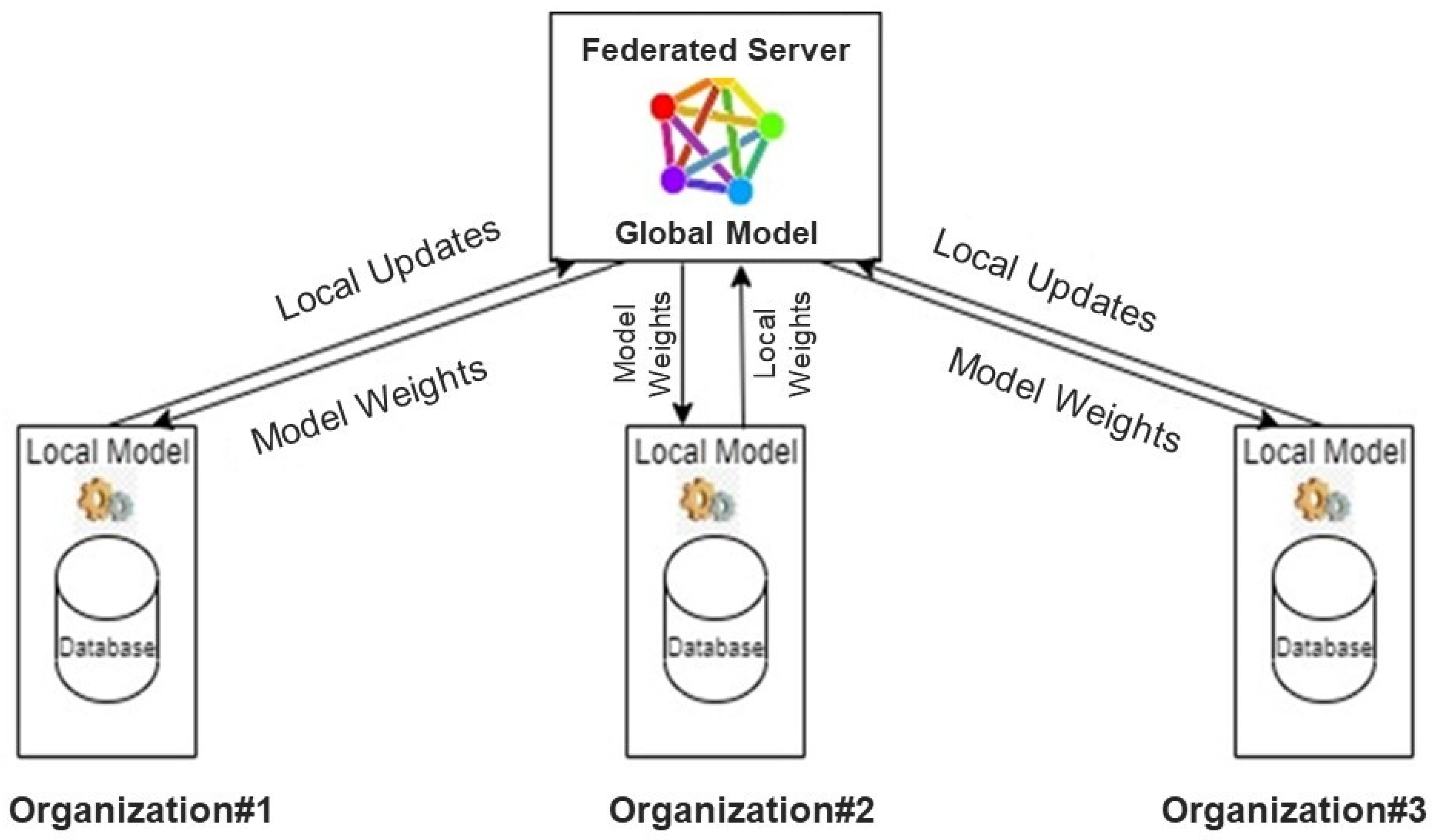
2.3. Federated Server


2.4. Optimal Weights of Hidden Output Layer


2.5. Proposed Weighted Federated Machine Learning Algorithm Pseudo Code
2.6. Edge Device
3. Simulations and Results
4. Discussion
Performance Analysis of The Weighted Federated Learning
5. Conclusions
Author Contributions
Funding
Institutional Review Board Statement
Informed Consent Statement
Data Availability Statement
Conflicts of Interest
References
- Preuster, P.; Alekseev, A.; Wasserscheid, P. Hydrogen storage technologies for future energy systems. Annu. Rev. Chem. Biomol. Eng. 2017, 8, 445–471. [Google Scholar] [CrossRef] [PubMed]
- Ali, A.; Rohini, A.K.; Noh, Y.S.; Moon, D.J.; Lee, H.J. Hydrogenation of dibenzyltoluene and the catalytic performance of Pt/Al2O3 with various Pt loadings for hydrogen production from perhydro-dibenzyltoluene. Int. J. Energy Res. 2022, 46, 6672–6688. [Google Scholar] [CrossRef]
- Ali, A.; Rohini, A.K.; Lee, H.J. Dehydrogenation of perhydro-dibenzyltoluene for hydrogen production in a microchannel reactor. Int. J. Hydrogen Energy 2022, 47, 20905–20914. [Google Scholar] [CrossRef]
- Niermann, M.; Drünert, S.; Kaltschmitt, M.; Bonhoff, K. Liquid organic hydrogen carriers (LOHCs)–techno-economic analysis of LOHCs in a defined process chain. Energy Environ. Sci. 2019, 12, 290–307. [Google Scholar] [CrossRef]
- Müller, K. Technologies for the Storage of Hydrogen Part 1: Hydrogen Storage in the Narrower Sense. ChemBioEng Rev. 2019, 6, 72–80. [Google Scholar] [CrossRef]
- Jang, M.; Jo, Y.S.; Lee, W.J.; Shin, B.S.; Sohn, H.; Jeong, H.; Jang, S.C.; Kwak, S.K.; Kang, J.W.; Yoon, C.W. A high-capacity, reversible liquid organic hydrogen carrier: H2-release properties and an application to a fuel cell. ACS Sustain. Chem. Eng. 2018, 7, 1185–1194. [Google Scholar] [CrossRef]
- Brückner, N.; Obesser, K.; Bösmann, A.; Teichmann, D.; Arlt, W.; Dungs, J.; Wasserscheid, P. Evaluation of Industrially applied heat-transfer fluids as liquid organic hydrogen carrier systems. ChemSusChem 2014, 7, 229–235. [Google Scholar] [CrossRef]
- Geburtig, D.; Preuster, P.; Bösmann, A.; Müller, K.; Wasserscheid, P. Chemical utilization of hydrogen from fluctuating energy sources—Catalytic transfer hydrogenation from charged Liquid Organic Hydrogen Carrier systems. Int. J. Hydrogen Energy 2016, 41, 1010–1017. [Google Scholar] [CrossRef] [Green Version]
- Geburtig, D. Transfer Hydrogenation Using Liquid Organic Hydrogen Carrier Systems as Hydrogen Source. Doctoral Dissertation, Friedrich-Alexander-Universität Erlangen-Nürnberg, Erlangen, Germany, 2019. [Google Scholar]
- Dürr, S.; Zilm, S.; Geißelbrecht, M.; Müller, K.; Preuster, P.; Bösmann, A.; Wasserscheid, P. Experimental determination of the hydrogenation/dehydrogenation-Equilibrium of the LOHC system H0/H18-dibenzyltoluene. Int. J. Hydrogen Energy 2021, 46, 32583–32594. [Google Scholar] [CrossRef]
- Feng, X.; Jiang, L.; Li, Z.; Wang, S.; Ye, J.; Wu, Y.; Yuan, B. Boosting the hydrogenation activity of dibenzyltoluene catalyzed by Mg-based metal hydrides. Int. J. Hydrogen Energy 2022, 47, 23994–24003. [Google Scholar] [CrossRef]
- Shi, L.; Qi, S.; Qu, J.; Che, T.; Yi, C.; Yang, B. Integration of hydrogenation and dehydrogenation based on dibenzyltoluene as liquid organic hydrogen energy carrier. Int. J. Hydrogen Energy 2019, 44, 5345–5354. [Google Scholar] [CrossRef]
- Sparks, T.D.; Gaultois, M.W.; Oliynyk, A.; Brgoch, J.; Meredig, B. Data mining our way to the next generation of thermoelectrics. Scr. Mater. 2016, 111, 10–15. [Google Scholar] [CrossRef]
- Yan, J.; Gorai, P.; Ortiz, B.; Miller, S.; Barnett, S.A.; Mason, T.; Stevanović, V.; Toberer, E.S. Material descriptors for predicting thermoelectric performance. Energy Environ. Sci. 2015, 8, 983–994. [Google Scholar] [CrossRef]
- Seshadri, R.; Sparks, T.D. Perspective: Interactive material property databases through aggregation of literature data. APL Mater. 2016, 4, 053206. [Google Scholar] [CrossRef] [Green Version]
- Oliynyk, A.O.; Antono, E.; Sparks, T.D.; Ghadbeigi, L.; Gaultois, M.W.; Meredig, B.; Mar, A. High-throughput machine-learning-driven synthesis of full-Heusler compounds. Chem. Mater. 2016, 28, 7324–7331. [Google Scholar] [CrossRef] [Green Version]
- Pilania, G.; Balachandran, P.V.; Gubernatis, J.E.; Lookman, T. Classification of ABO3 perovskite solids: A machine learning study. Acta Crystallogr. Sect. B Struct. Sci. Cryst. Eng. Mater. 2015, 71, 507–513. [Google Scholar] [CrossRef]
- Pilania, G.; Balachandran, P.V.; Kim, C.; Lookman, T. Finding new perovskite halides via machine learning. Front. Mater. 2016, 3, 19. [Google Scholar] [CrossRef] [Green Version]
- Balachandran, P.V.; Broderick, S.R.; Rajan, K. Identifying the ‘inorganic gene’ for high-temperature piezoelectric perovskites through statistical learning. Proc. R. Soc. A Math. Phys. Eng. Sci. 2011, 467, 2271–2290. [Google Scholar] [CrossRef] [Green Version]
- Pilania, G.; Mannodi-Kanakkithodi, A.; Uberuaga, B.P.; Ramprasad, R.; Gubernatis, J.E.; Lookman, T. Machine learning bandgaps of double perovskites. Sci. Rep. 2016, 6, 1–10. [Google Scholar] [CrossRef] [Green Version]
- Wilmer, C.E.; Leaf, M.; Lee, C.Y.; Farha, O.K.; Hauser, B.G.; Hupp, J.T.; Snurr, R.Q. Large-scale screening of hypothetical metal–organic frameworks. Nat. Chem. 2012, 4, 83–89. [Google Scholar] [CrossRef]
- Lin, L.C.; Berger, A.H.; Martin, R.L.; Kim, J.; Swisher, J.A.; Jariwala, K.; Rycroft, C.H.; Bhown, A.S.; Deem, M.W.; Haranczyk, M.; et al. In silico screening of carbon-capture materials. Nat. Mater. 2012, 11, 633–641. [Google Scholar] [CrossRef] [PubMed] [Green Version]
- Greeley, J.; Jaramillo, T.F.; Bonde, J.; Chorkendorff, I.B.; Nørskov, J.K. Computational high-throughput screening of electrocatalytic materials for hydrogen evolution. Nat. Mater. 2006, 5, 909–913. [Google Scholar] [CrossRef] [PubMed]
- Hong, W.T.; Welsch, R.E.; Shao-Horn, Y. Descriptors of oxygen-evolution activity for oxides: A statistical evaluation. J. Phys. Chem. C 2016, 120, 78–86. [Google Scholar] [CrossRef]
- Kim, E.; Huang, K.; Tomala, A.; Matthews, S.; Strubell, E.; Saunders, A.; McCallum, A.; Olivetti, E. Machine-learned and codified synthesis parameters of oxide materials. Sci. Data 2017, 4, 1–9. [Google Scholar] [CrossRef] [Green Version]
- Sumpter, B.G.; Vasudevan, R.K.; Potok, T.; Kalinin, S.V. A bridge for accelerating materials by design. NPJ Comput. Mater. 2015, 1, 1–11. [Google Scholar] [CrossRef] [Green Version]
- Kalinin, S.V.; Sumpter, B.G.; Archibald, R.K. Big–deep–smart data in imaging for guiding materials design. Nat. Mater. 2015, 14, 973–980. [Google Scholar] [CrossRef]
- Kim, E.; Huang, K.; Jegelka, S.; Olivetti, E. Virtual screening of inorganic materials synthesis parameters with deep learning. NPJ Comput. Mater. 2017, 3, 1–9. [Google Scholar] [CrossRef] [Green Version]
- Rahnama, A.; Clark, S.; Sridhar, S. Machine learning for predicting occurrence of interphase precipitation in HSLA steels. Comput. Mater. Sci. 2018, 154, 169–177. [Google Scholar] [CrossRef]
- Gómez-Bombarelli, R.; Aguilera-Iparraguirre, J.; Hirzel, T.D.; Duvenaud, D.; Maclaurin, D.; Blood-Forsythe, M.A.; Chae, H.S.; Einzinger, M.; Ha, D.G.; Wu, T.; et al. Design of efficient molecular organic light-emitting diodes by a high-throughput virtual screening and experimental approach. Nat. Mater. 2016, 15, 1120–1127. [Google Scholar] [CrossRef]
- Dashti, A.; Harami, H.R.; Rezakazemi, M. Accurate prediction of solubility of gases within H2-selective nanocomposite membranes using committee machine intelligent system. Int. J. Hydrogen Energy 2018, 43, 6614–6624. [Google Scholar] [CrossRef]
- Rezakazemi, M.; Dashti, A.; Asghari, M.; Shirazian, S. H2-selective mixed matrix membranes modeling using ANFIS, PSO-ANFIS, GA-ANFIS. Int. J. Hydrogen Energy 2017, 42, 15211–15225. [Google Scholar] [CrossRef]
- Rezakazemi, M.; Azarafza, A.; Dashti, A.; Shirazian, S. Development of hybrid models for prediction of gas permeation through FS/POSS/PDMS nanocomposite membranes. Int. J. Hydrogen Energy 2018, 43, 17283–17294. [Google Scholar] [CrossRef]
- Rahnama, A.; Zepon, G.; Sridhar, S. Machine learning based prediction of metal hydrides for hydrogen storage, part I: Prediction of hydrogen weight percent. Int. J. Hydrogen Energy 2019, 44, 7337–7344. [Google Scholar] [CrossRef]
- Rahnama, A.; Zepon, G.; Sridhar, S. Machine learning based prediction of metal hydrides for hydrogen storage, part II: Prediction of material class. Int. J. Hydrogen Energy 2019, 44, 7345–7353. [Google Scholar] [CrossRef]
- Ahmed, A.; Seth, S.; Purewal, J.; Wong-Foy, A.G.; Veenstra, M.; Matzger, A.J.; Siegel, D.J. Exceptional hydrogen storage achieved by screening nearly half a million metal-organic frameworks. Nat. Commun. 2019, 10, 1–9. [Google Scholar] [CrossRef] [PubMed] [Green Version]
- Abad, G.; Picek, S.; Urbieta, A. SoK: On the Security & Privacy in Federated Learning. arXiv 2021, arXiv:2112.05423. [Google Scholar]
- Federated Learning: Predictive Model Without Data Sharing–Sparkd AI. Available online: https://sparkd.ai/federated-learning (accessed on 28 August 2022).
- Oueida, S.; Kotb, Y.; Aloqaily, M.; Jararweh, Y.; Baker, T. An edge computing based smart healthcare framework for resource management. Sensors 2018, 18, 4307. [Google Scholar] [CrossRef] [Green Version]
- Ata, A.; Khan, M.A.; Abbas, S.; Ahmad, G.; Fatima, A. Modelling smart road traffic congestion control system using machine learning techniques. Neural Netw. World 2018, 29, 99–110. [Google Scholar] [CrossRef] [Green Version]
- Rehman, A.; Athar, A.; Khan, M.A.; Abbas, S.; Fatima, A.; Saeed, A. Modelling, simulation, and optimization of diabetes type II prediction using deep extreme learning machine. J. Ambient. Intell. Smart Environ. 2020, 12, 125–138. [Google Scholar] [CrossRef]
- Khan, A.H.; Khan, M.A.; Abbas, S.; Siddiqui, S.Y.; Saeed, M.A.; Alfayad, M.; Elmitwally, N.S. Simulation, modeling, and optimization of intelligent kidney disease predication empowered with computational intelligence approaches. CMC-Comput. Mater. Continua 2021, 67, 1399–1412. [Google Scholar] [CrossRef]
- Khan, M.A.; Abbas, S.; Rehman, A.; Saeed, Y.; Zeb, A.; Uddin, M.I.; Nasser, N.; Ali, A. A machine learning approach for blockchain-based smart home networks security. IEEE Netw. 2020, 35, 223–229. [Google Scholar] [CrossRef]
- Khan, M.A.; Abbas, S.; Atta, A.; Ditta, A.; Alquhayz, H.; Khan, M.F.; Naqvi, R.A. Intelligent cloud based heart disease prediction system empowered with supervised machine learning. CMC-Comput. Mater. Continua 2020, 65, 139–151. [Google Scholar] [CrossRef]
- Mehmood, S.; Ghazal, T.M.; Khan, M.A.; Zubair, M.; Naseem, M.T.; Faiz, T.; Ahmad, M. Malignancy Detection in Lung and Colon Histopathology Images Using Transfer Learning With Class Selective Image Processing. IEEE Access 2022, 10, 25657–25668. [Google Scholar] [CrossRef]
- Thornton, A.W.; Simon, C.M.; Kim, J.; Kwon, O.; Deeg, K.S.; Konstas, K.; Pas, S.J.; Hill, M.R.; Winkler, D.A.; Haranczyk, M.; et al. Materials genome in action: Identifying the performance limits of physical hydrogen storage. Chem. Mater. 2017, 29, 2844–2854. [Google Scholar] [CrossRef]
- Bucior, B.J.; Bobbitt, N.S.; Islamoglu, T.; Goswami, S.; Gopalan, A.; Yildirim, T.; Farha, O.K.; Bagheri, N.; Snurr, R.Q. Energy-based descriptors to rapidly predict hydrogen storage in metal–organic frameworks. Mol. Syst. Des. Eng. 2019, 4, 162–174. [Google Scholar] [CrossRef]
- Hastie, T.; Tibshirani, R.; Friedman, J.H.; Friedman, J.H. The Elements of Statistical Learning: Data Mining, Inference, and Prediction; Springer: New York, NY, USA, 2009; pp. 1–758. [Google Scholar]


| Client Training Algorithm (, ) 1. Start 2. Local data splitting to small groups of size Cs 3. Initialize both layers i.e., input layer and hidden layer weights ((, )), = 0 and number of epochs d = 0 4. For every small group (Cs) i. Apply the feedforward phase to a. Calculate using Equation (4) b. Calculate estimated output ()using Equation (5) ii. Calculate the Error values using Equation (6) iii. weights updating phase a. Calculate using Equation (13) b. Calculate using Equation (18) c. Update the weights between hidden and output layers using Equation (20) d. Update the weights between input and hidden layers using Equation (21) if stopping Criteria do not meet, then go to step 4 else, go to step 5 5. Return optimum weights (, ) to Federated Server Stop |
| 1. Start 2. Initialize weights ) 3. For each cycle Do for each client Do ) End End 4. Calculate using Equation (47) 5. Calculate using Equation (34) 6. Prediction of unknown data samples a. for I = No. of Samples i. Calculate ii. Calculate iii. Calculate error 7. Stop |
| Low Class | Medium Class | High Class | |
|---|---|---|---|
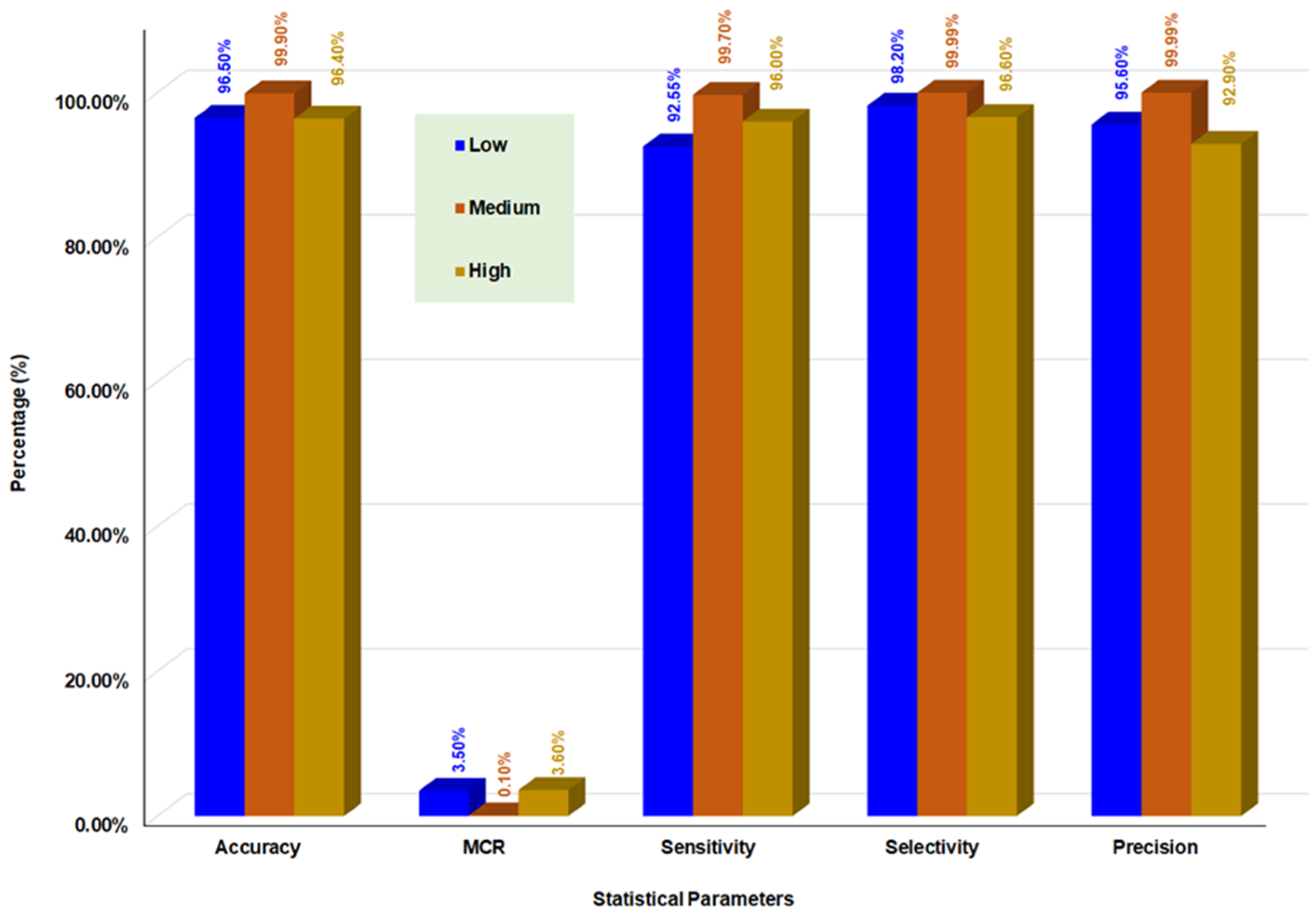
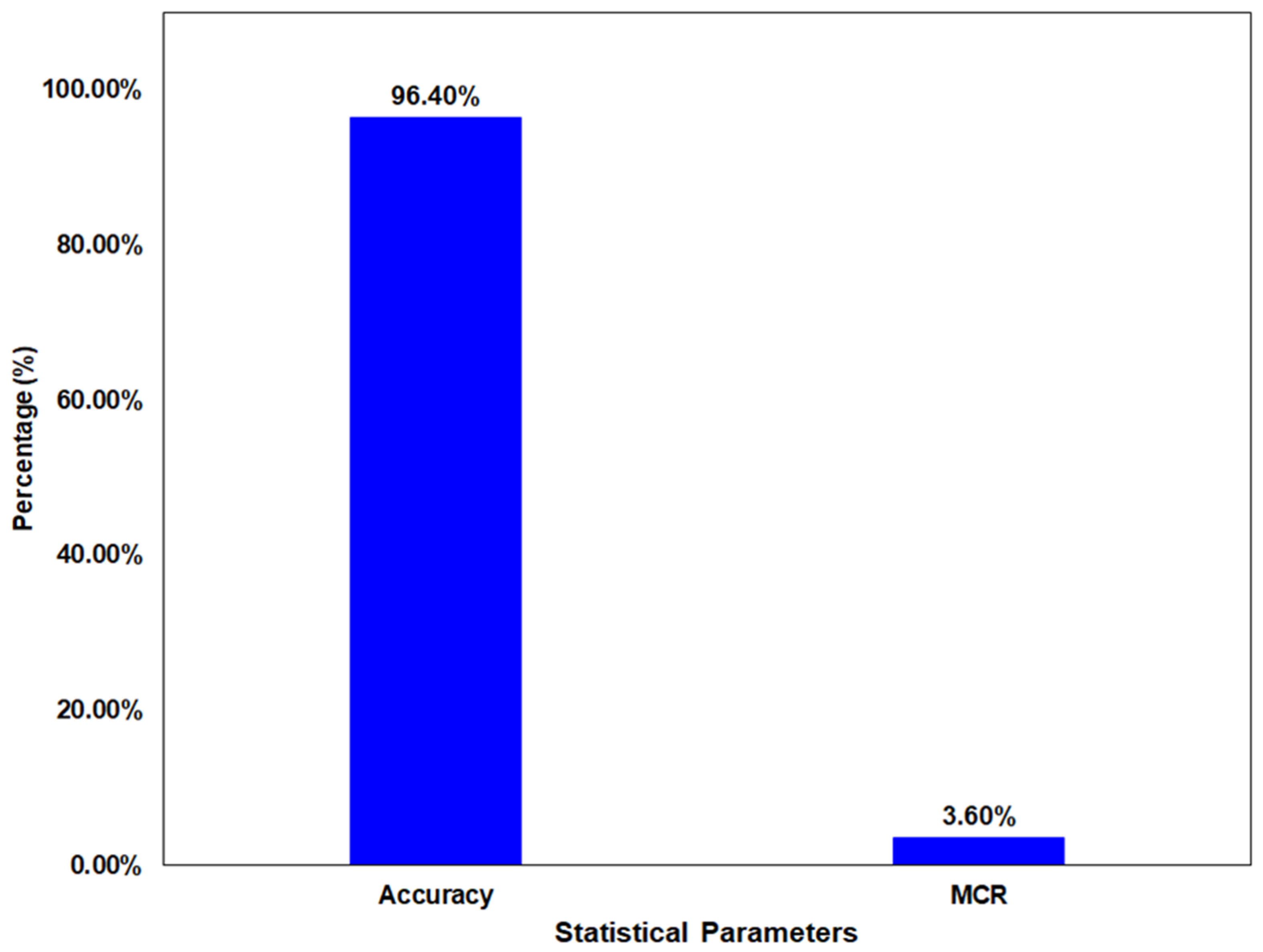
| Accuracy | 96.50% | 99.90% | 96.40% |
| Misclassification Rate | 3.50% | 0.10% | 3.60% |
| Recall/Sensitivity | 92.55% | 99.70% | 96.00% |
| Selectivity | 98.20% | 99.99% | 96.60% |
| Precision | 95.60% | 99.99% | 92.90% |
| False Omission Rate | 3.15% | 0.16% | 1.90% |
| False Discovery Rate | 4.40% | 0.001% | 7.10% |
| F0.5 Score | 95.00% | 99.95% | 93.50% |
| F1 Score | 94.10% | 99.85% | 94.40% |
| Studies | Year | Storage System | Model | Accuracy |
|---|---|---|---|---|
| Thornton et al. [46] | 2017 | Nanoporous materials | Neural network | 88.00% |
| Rahnama et al. [34] | 2019 | Metal hydrides | Boosted decision tree regression | 83.00% |
| Rahnama et al. [35] | 2019 | Metal hydrides | Multi-class neural network | 80.00% |
| Bucior et al. [47] | 2019 | Metal organic frameworks | Multi-linear regression with LASSO [48] | 96.00% |
| Ahsan et al. | Current work | LOHC | HSPS-WFML | 96.40% |
Publisher’s Note: MDPI stays neutral with regard to jurisdictional claims in published maps and institutional affiliations. |
© 2022 by the authors. Licensee MDPI, Basel, Switzerland. This article is an open access article distributed under the terms and conditions of the Creative Commons Attribution (CC BY) license (https://creativecommons.org/licenses/by/4.0/).
Share and Cite
Ali, A.; Khan, M.A.; Choi, H. Hydrogen Storage Prediction in Dibenzyltoluene as Liquid Organic Hydrogen Carrier Empowered with Weighted Federated Machine Learning. Mathematics 2022, 10, 3846. https://doi.org/10.3390/math10203846
Ali A, Khan MA, Choi H. Hydrogen Storage Prediction in Dibenzyltoluene as Liquid Organic Hydrogen Carrier Empowered with Weighted Federated Machine Learning. Mathematics. 2022; 10(20):3846. https://doi.org/10.3390/math10203846
Chicago/Turabian StyleAli, Ahsan, Muhammad Adnan Khan, and Hoimyung Choi. 2022. "Hydrogen Storage Prediction in Dibenzyltoluene as Liquid Organic Hydrogen Carrier Empowered with Weighted Federated Machine Learning" Mathematics 10, no. 20: 3846. https://doi.org/10.3390/math10203846